A Bearing Fault Detection Method Based on EMDWS-CNT-BO

Abstract

Accurate diagnosis of bearing faults is crucial for ensuring the safe and reliable operation of rotating machinery. To enhance the recognition accuracy of rolling bearings under nonlinear and non-stationary vibration conditions, this study proposes an integrated approach combining a multi-stage signal preprocessing strategy, termed EMDWS (Empirical Mode Decomposition with Wavelet denoising and SMOTE), with a hybrid deep learning architecture that integrates a Convolutional Neural Network (CNN) and a Transformer model, hereinafter referred to as CNT (CNN-Transformer). The method first applies empirical mode decomposition (EMD) in conjunction with wavelet denoising to enhance the representation of non-stationary fault features. Subsequently, the synthetic minority oversampling technique (SMOTE) is employed to address the issue of class imbalance in the dataset. A hybrid CNN-Transformer model is constructed by integrating convolutional neural networks and Transformer modules, enabling the extraction of both local and global signal characteristics. Furthermore, Bayesian optimization is applied to fine-tune the model’s hyperparameters, thereby enhancing both the efficiency and robustness of the model. Experimental results demonstrate that the proposed method achieves a high identification accuracy of 99.83%, indicating its effectiveness in distinguishing various bearing fault types.

1. Introduction

In modern industrial applications, rotating machinery is a core asset, with rolling bearings as one of its most critical components. Mechanical failures of rolling bearings are a common issue that can lead to motor malfunctions, reduced production efficiency, and even severe safety incidents [1,2]. Therefore, developing efficient and accurate fault diagnosis methods is of paramount importance. Such methods enable the prompt identification and localization of system anomalies, preventing further damage and thereby improving system reliability while reducing maintenance costs [3,4].

In the diagnostic process, extracting effective fault information from raw signals encounters two primary challenges: severe background noise interference and the limited availability of fault samples under real-world operating conditions. To overcome these challenges, researchers have employed a range of data preprocessing techniques. For instance, in the field of filtering technology, empirical mode decomposition (EMD) [5] has been widely applied, although it suffers from limitations such as mode aliasing. To address this issue, ensemble empirical mode decomposition (EEMD) [6,7] was developed as an improved variant capable of further decomposing high-frequency signal components. Other advanced methods include wavelet packet transform (WPT) [8] and empirical wavelet transform (EWT) [9,10], the latter of which integrates the concepts of wavelet transform and empirical mode decomposition to enable adaptive frequency band partitioning for signal decomposition.

As the volume of collected data continues to grow, the feature signals extracted from raw data often contain redundant noise and suffer from poor sample quality, which can negatively affect subsequent model training and analytical outcomes [11]. Therefore, the application of denoising techniques constitutes a critical step in the diagnostic process. Signal decomposition approaches, with wavelet transform (WT) as a representative example, have been extensively utilized to suppress noise and highlight fault-related features. Wavelet threshold denoising leverages multi-scale decomposition to simultaneously capture both time and frequency features of the signal. This makes it particularly effective in handling non-stationary data, especially those with abrupt changes [12,13]. Meanwhile, to effectively address the issue of class imbalance resulting from insufficient fault data, algorithms such as the Synthetic Minority Over-sampling Technique (SMOTE) have emerged as widely adopted data augmentation strategies [14]. For instance, Wang et al. [15] effectively combined an improved SMOTE model with a CNN to tackle imbalanced bearing data, underscoring the importance of this preprocessing step. However, the majority of existing studies apply these techniques in a fragmented manner, without establishing a comprehensive, multi-phase preprocessing framework capable of addressing both poor signal quality and sample imbalance issues in a coordinated manner.

In the feature extraction and classification phase, deep learning models, with convolutional neural networks (CNNs) as a representative example, have gained widespread adoption owing to their capability to automatically extract discriminative features and effectively capture local patterns. For instance, Yang et al. [16] proposed an interpretable intelligent fault diagnosis framework to address the black-box issue caused by mixed feature decisions in standard CNNs for rotating machinery fault diagnosis, achieving both fault signal recognition and visual interpretation of model features. Reference [3] proposes a deeply integrated framework termed SKND-TSACNN, which effectively integrates Time-Scale Adaptive CNN (TSACNN) and Neural Denoiser (SKND). The proposed framework is specifically designed to overcome the limitations of traditional CNN models, including low diagnostic accuracy and insufficient noise resistance, particularly under complex operational conditions and in the presence of significant noise interference. Zhong et al. [17] proposed a remaining useful life prediction method for rolling bearings based on an improved convolutional bidirectional gated recurrent unit neural network (CNN-BGRU), which significantly enhanced the accuracy of predicting remaining useful life compared to existing AI-based approaches. CNNs offer advantages such as translation-invariant classification, weight sharing, and efficient convolution operations [18]. However, due to the limitation of their local receptive fields [19], modeling long-range dependencies remains challenging [20,21]. To address this limitation, researchers have increasingly explored the application of the Transformer framework in fault diagnosis. Initially developed for natural language processing (NLP) [22], the Transformer has since been extended to various domains, including computer vision, multimodal learning, industrial monitoring, and fault diagnosis. In [23], a rolling bearing fault diagnosis method was proposed that integrates sub-domain adaptation (SA) with an improved visual Transformer network (IVTN), effectively combining local and global information to achieve high-precision fault diagnosis under variable-speed and variable-load conditions. In [24], a self-supervised learning (SSL) approach incorporating a self-attention mechanism was introduced, leveraging the Transformer architecture to enhance temporal feature learning and global modeling, thereby improving diagnostic performance under novel operating conditions. In [25], a PRT model based on the Transformer was proposed, utilizing dense overlapping splitting and a class attention mechanism to improve feature learning. Li et al. [26] introduced a variational attention mechanism into the Transformer architecture to better capture the correlation among vibration signals in rotating machinery fault diagnosis and to enhance model interpretability. However, transformer models generally necessitate large-scale datasets for effective training, and the optimization process entails substantial computational resources, thereby restricting their deployment in real-world industrial applications.

To overcome the limitations of CNNs in modeling long-range dependencies and to reduce the high computational complexity associated with Transformers, researchers have developed CNN-Transformer hybrid architectures [27]. These models effectively integrate the local feature extraction capability of CNNs with the global modeling strengths of Transformers. The C-ECAFormer architecture proposed by Wang et al. combines the spatial sensitivity of CNNs with the global attention mechanism of Transformers, achieving robust fault diagnosis performance under conditions of strong noise and limited sample sizes [28]. In [29], a multi-task CNN-Transformer (MT-ConvFormer) method was proposed for bearing fault diagnosis, addressing key challenges in current intelligent diagnosis approaches, including the limited exploration of multi-fault task analysis and the challenge of capturing complementary fault characteristics. This method also enhances diagnostic performance under noisy environments and in cases of imbalanced data distribution. Fang et al. proposed the CLFormer architecture, enhancing the resilience and precision of Transformers in the context of bearing fault identification by incorporating convolutional embedding and a linear self-attention mechanism (LSA) [30]. Although these hybrid approaches partially mitigate the limitations of both CNNs and Transformers, they still face challenges such as performance redundancy and limited engineering adaptability due to complex network structures. Furthermore, while previous studies have explored individual components of our proposed framework—such as the CNN-Transformer architecture for multi-task learning [29], the use of SMOTE with CNNs for imbalanced data [15], and the application of Bayesian optimization to standard CNNs [31]—they often focus on improving a single stage of the diagnostic pipeline.

A systematic integration that synergistically combines advanced signal preprocessing, a hybrid feature extractor, and intelligent hyperparameter optimization for such a complex architecture remains underexplored. Therefore, building upon the CNN-Transformer hybrid framework, this study innovatively incorporates two critical components—a comprehensive data preprocessing pipeline (EMDWS) and an automated hyperparameter optimization strategy (BO)—aiming to create a holistic, end-to-end diagnostic solution. This integrated approach not only mitigates the practical application challenges of existing hybrid models but also enhances diagnostic accuracy and robustness under complex conditions such as strong noise and limited sample sizes, providing a more engineering-feasible solution for the efficient fusion of CNN and Transformer architectures.

The principal contributions of this study are delineated as follows:

(1) We propose a holistic preprocessing framework, EMDWS, that systematically integrates EMD, Wavelet Denoising, and SMOTE to simultaneously address the dual challenges of poor signal quality and data imbalance in complex conditions.

(2) We validate the synergistic effect between a hybrid CNN-Transformer architecture and Bayesian Optimization (BO), demonstrating that BO is a critical component—not merely an add-on—for maximizing the diagnostic performance of such a complex model.

(3) We present and validate an end-to-end automated diagnostic pipeline, EMDWS-CNT-BO. Experiments on multiple datasets prove that this systematically integrated framework is significantly superior to baseline models that lack either comprehensive preprocessing or hyperparameter optimization.

2. Related Work and Theoretical Background

This chapter begins by presenting the core methodologies employed in this study, specifically Empirical Mode Decomposition (EMD), wavelet threshold denoising, SMOTE oversampling technique, and the fundamental architecture of deep learning models. Following this, a comprehensive comparison and critical analysis of prevailing signal processing approaches are conducted to substantiate the necessity and superiority of the proposed methodological framework.

2.1. Background of Core Techniques

2.1.1. Empirical Mode Decomposition

Empirical Mode Decomposition (EMD) is an adaptive signal analysis method, particularly effective for processing nonlinear and non-stationary data. Its core function is to decompose a complex signal $x\left(t\right)$ into a finite series of Intrinsic Mode Functions (IMFs), $c_i\left(t\right)$, plus a final residual $r_n\left(t\right)$ [32]. Each IMF represents a distinct oscillatory mode embedded within the signal. The original signal can be perfectly reconstructed by summing these components [33,34].

$$x\left(t\right) = \sum _{i = 1}^n{c}_i\left(t\right) + r_n\left(t\right)$$

(1)

This data-driven decomposition allows for a detailed multi-scale analysis of the original signal’s characteristics.

2.1.2. Wavelet Threshold Denoising

Wavelet threshold denoising is an effective technique for signal purification. The method achieves noise reduction by transforming the signal into the wavelet domain and applying thresholding to the wavelet coefficients associated with noise components. This study employs the hard thresholding function, which is mathematically defined as:

$${\widehat{d}}_{j,k} = \left\{\begin{array}{cc}{d}_{j,k},\hfill & |d_{j,k}| \ge \lambda \hfill \\ 0,\hfill & |d_{j,k}| < \lambda \hfill \end{array}\right.$$

(2)

Specifically, $d_{j,k}$ denotes the original wavelet detail coefficient, $\lambda$ represents the threshold value, and ${\widehat{d}}_{j,k}$ signifies the processed coefficient. The denoised signal is reconstructed by applying the inverse wavelet transform to the processed coefficients. By applying this process to each IMF component from EMD, we can achieve more targeted and effective noise suppression [35,36].

2.1.3. SMOTE for Data Imbalance

Sample imbalance is a common challenge in fault diagnosis that can lead to biased models. To address this, the Synthetic Minority Over-sampling Technique (SMOTE) is employed [37,38]. SMOTE generates new, synthetic samples for the minority class. For each minority sample $x_i$, it randomly selects one of its k-nearest neighbors, ${\tilde{x}}_i$, and creates a new sample $x_{\mathrm{new}}$ along the line segment connecting the two.

$$x_{\mathrm{new}} = x_i + \lambda · (x_n - x_i),\lambda \sim U(0,1)$$

(3)

where $\lambda$ is a random number between 0 and 1, which controls the distance between the synthetic sample and the original sample.This approach effectively enlarges the decision region for the minority class and improves the model’s ability to recognize rare fault types.

2.1.4. Convolutional Neural Network Architecture

A Convolutional Neural Network (CNN) is a deep learning architecture adept at automatically extracting hierarchical features. Its fundamental operation occurs in the convolutional layer, where learnable filters (or kernels) K are slid across the input X to produce feature maps [39]. This process, which captures local patterns, can be mathematically defined as:

$$Y = f(X\ast K + b_c)$$

(4)

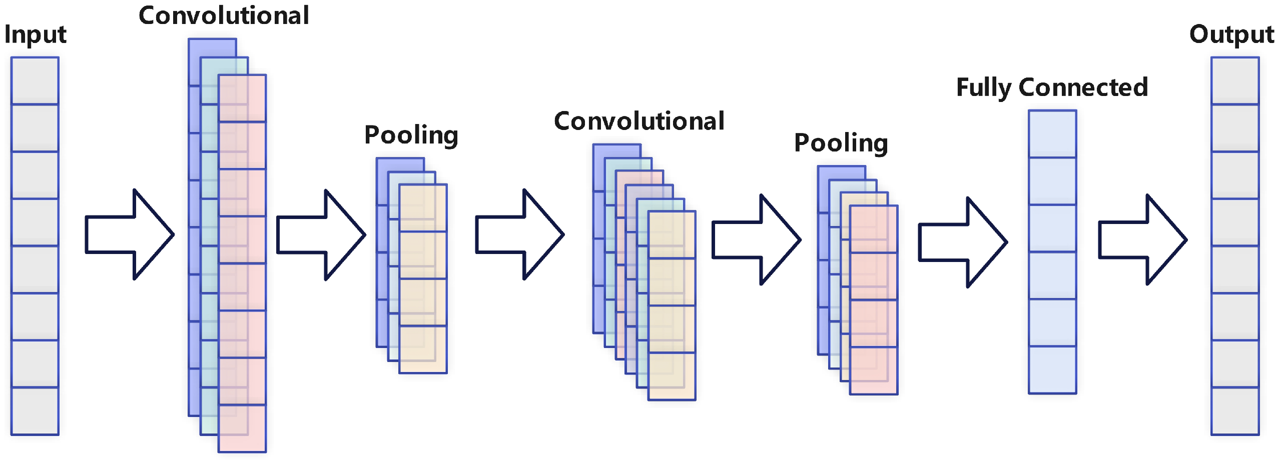
Here, * denotes the convolution operation, $b_c$ is a bias term, and f is a non-linear activation function like ReLU.Through stacking these layers with pooling operations, CNNs can efficiently learn discriminative local features for classification, as illustrated in Figure 1.

The feature extraction in a CNN is typically performed by a series of convolutional blocks. Each block applies three sequential operations to its input data: convolution, activation, and pooling.

2.1.5. Transformer Architecture

The Transformer architecture excels at modeling long-range dependencies via its self-attention mechanism. This mechanism allows the model to weigh the importance of all other positions when encoding a specific position. It operates on queries (Q), keys (K), and values (V) projected from the input [40]. The core computation is the scaled dot-product attention:

$$\mathrm{Attention}(Q,K,V) = \mathrm{softmax}\left({\displaystyle \frac{Q{K}^T}{\sqrt{d_k}}}\right)V$$

(5)

where $d_k$ is the dimension of the keys. By running multiple such attention functions in parallel (“multi-head attention”), the Transformer can capture complex, global relationships within the data.

2.1.6. Bayesian Hyperparameter Optimization

Bayesian Optimization is an efficient global optimization strategy for hyperparameter tuning. It builds a probabilistic surrogate model of the objective function and uses an acquisition function to intelligently select the next hyperparameters to evaluate [41]. A widely used acquisition function is Expected Improvement (EI), which quantifies the expected improvement over the current best-observed value $f\left({\mathbf{x}}^{+}\right)$:

$$\mathrm{EI}\left(\mathbf{x}\right) = \mathbb{E}[max(0,f\left(\mathbf{x}\right) - f\left({\mathbf{x}}^{+}\right))]$$

(6)

By maximizing this function at each step, BO effectively balances exploring uncertain regions of the parameter space and exploiting regions known to yield good performance, thus finding near-optimal solutions with fewer evaluations.

2.2. Comparison and Selection of Signal Preprocessing Methods

To determine the optimal preprocessing strategy for this study, a comprehensive evaluation and comparative analysis were conducted on various mainstream signal processing methods.

Although the classical Fourier Transform (FT) demonstrates effectiveness in analyzing the frequency-domain characteristics of stationary signals, its inherent global transformation mechanism prevents it from providing time-localized information. Consequently, FT is not well-suited for the analysis of non-stationary signals exhibiting transient impact features, such as those observed in bearing fault diagnostics [42].

Wavelet Transform (WT) possesses multi-scale analysis capabilities, enabling simultaneous extraction of time-frequency information, which makes it particularly suitable for processing non-stationary signals. Nevertheless, the effectiveness of WT is heavily reliant on the choice of the pre-selected wavelet basis function. Given the diversity of fault signals, identifying a universally optimal wavelet basis remains a significant challenge, thereby constraining the method’s adaptability.

To enhance adaptability, Empirical Mode Decomposition (EMD) has gained widespread application due to its data-driven characteristics and the absence of predefined basis functions. Nevertheless, conventional EMD is inherently prone to the issue of mode mixing. To mitigate this limitation, Ensemble Empirical Mode Decomposition (EEMD) and its advanced variant, Complementary Ensemble Empirical Mode Decomposition (CEEMD), have been proposed. These approaches improve mode separation by incorporating auxiliary white noise [31]. While techniques such as CEEMD significantly reduce mode mixing, they are generally associated with increased computational complexity, and their effectiveness remains sensitive to the noise injection strategy and parameter configurations.

In recent years, Variational Mode Decomposition (VMD) has emerged as a promising signal decomposition technique, exhibiting robust anti-noise performance and a rigorous mathematical theoretical framework. However, the effectiveness of VMD is critically dependent on the proper initialization of two key parameters: the number of decomposition modes (K) and the penalty factor ($\alpha$). In practical applications, improper parameter selection may result in either over-decomposition or under-decomposition, which can compromise the accuracy of fault feature extraction [8].

Given the strengths and limitations of the aforementioned methods, the development of a collaborative strategy that integrates the fully adaptive nature of Empirical Mode Decomposition (EMD) with the precise noise reduction capability of Wavelet Transform (WT), while circumventing the parameter-setting dependency inherent in approaches such as Variational Mode Decomposition (VMD), represents a highly promising research direction. This consideration fundamentally motivates the proposal of the EMDWS framework in the present study.

3. The Proposed Approach

To address the signal processing challenges identified in Section 2 and fulfill the critical requirements for adaptability, accuracy, and robustness in diagnostic modeling, this study proposes and establishes an end-to-end, systematically integrated framework for rolling bearing fault diagnosis, termed EMDWS-CNT-BO. Unlike conventional approaches that merely stack individual techniques, the proposed framework is designed as a synergistically optimized and cohesive system, comprising three core components: (1) the EMDWS collaborative signal preprocessing module; (2) the CNT (CNN-Transformer) hybrid feature extraction module; and (3) the Bayesian hyperparameter intelligent optimization module.

3.1. The EMDWS Synergistic Signal Preprocessing Module

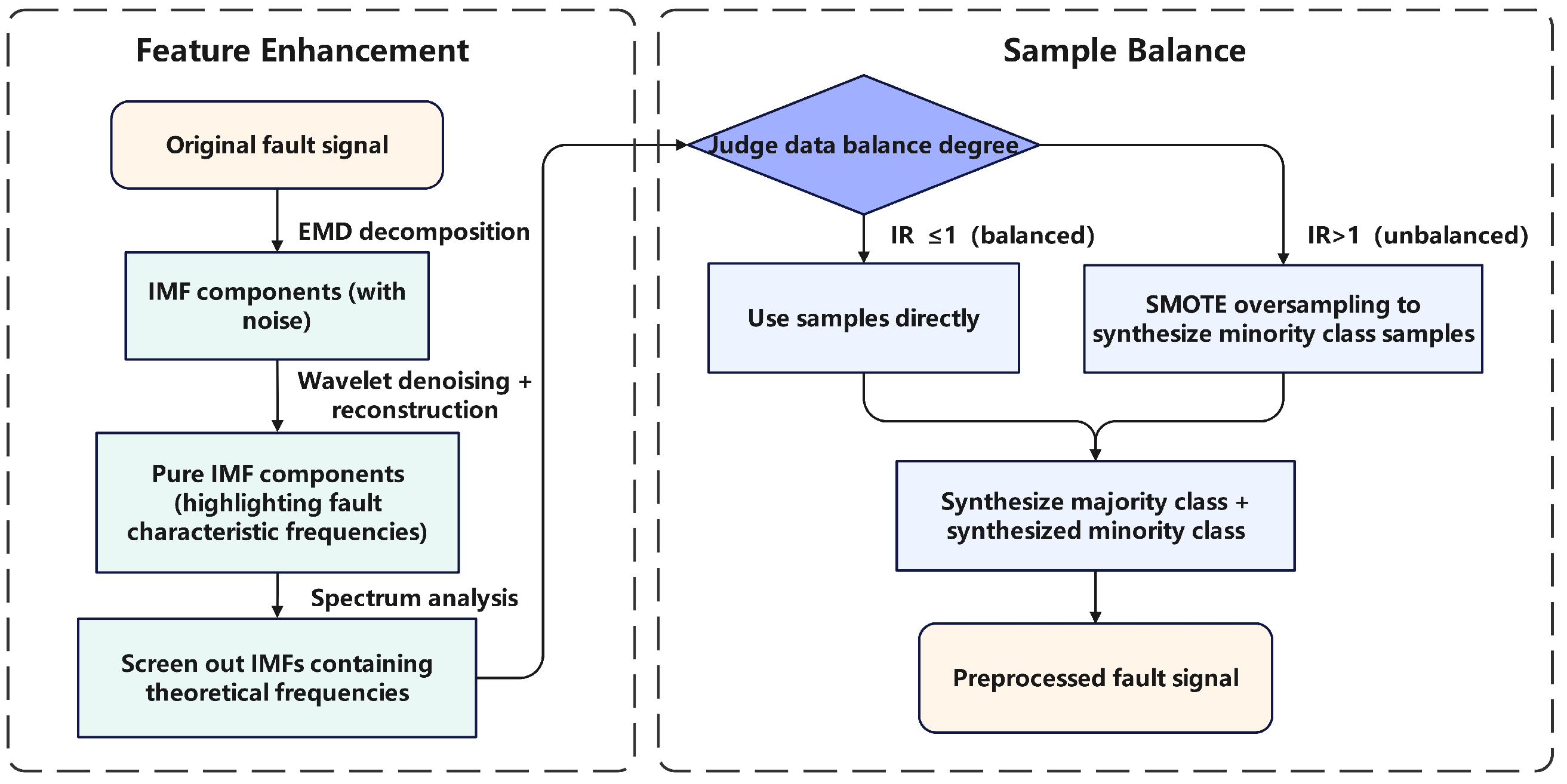
To tackle the two primary challenges—low signal-to-noise ratio in raw vibration signals and imbalanced fault sample distribution—this study proposes the EMDWS preprocessing pipeline. The objective of this pipeline is to generate a high-quality dataset characterized by enhanced feature representation and balanced class distribution, thereby facilitating improved performance of downstream deep learning models. The detailed processing steps are illustrated in Figure 2 and are elaborated below:

Stage 1: Adaptive Signal Decomposition

The process initiates with the original non-stationary vibration signal $x\left(t\right)$. Utilizing the fully data-driven nature of Empirical Mode Decomposition (EMD), the signal is adaptively decomposed into a sequence of Intrinsic Mode Functions (IMFs) ordered from high frequency to low frequency, denoted as $\{c_1\left(t\right),c_2\left(t\right),\dots ,c_k\left(t\right)\}$. This decomposition requires no predefined basis functions or parameters, thereby ensuring its applicability across diverse operating conditions.

Stage 2: IMF Screening and Targeted Denoising IMF

To ensure the validity of the decomposition, we screen the resulting Intrinsic Mode Functions (IMFs), discarding samples that yield fewer than seven IMFs as required by this study. Following this, to further purify the signal, wavelet threshold denoising is independently applied to each screened IMF, $c_i\left(t\right)$. For this stage, we utilized the db8 wavelet basis with a 3-level decomposition and applied a Donoho universal hard threshold for noise suppression. Owing to the more homogeneous characteristics of IMFs compared to the original signal, this wavelet-based approach can effectively suppress noise while preserving critical information associated with fault features. This process results in a set of denoised IMF components, $\{c_1^{\prime }\left(t\right),c_2^{\prime }\left(t\right),\dots ,c_n^{\prime }\left(t\right)\}$.

Stage 3: Data Balancing

Finally, to mitigate the adverse effects of data imbalance on model training, the Synthetic Minority Over-sampling Technique (SMOTE) is applied to the training set consisting of pure Intrinsic Mode Functions (IMFs). By generating synthetic samples within the feature space of minority class instances, SMOTE effectively increases their representation, thereby ensuring balanced data exposure during the training process and preventing the model from developing a bias toward the majority class.

Figure 2. Flowchart of the EMDWS Preprocessing Procedure.

Figure 2. Flowchart of the EMDWS Preprocessing Procedure.

3.2. The CNN-Transformer Hybrid Feature Extraction Model

The integration of CNN and Transformer architectures enables complementary advantages. Convolutional Neural Networks (CNNs) possess translation invariance and localized receptive fields, making them highly effective at identifying local patterns in signals—such as edges, textures, or transient features. In contrast, the self-attention mechanism of the Transformer exhibits strong global perception capabilities, enabling the capture of long-range dependencies across any positions in a sequence. A hybrid design, as depicted in Figure 3, typically employs the initial layers of CNN to rapidly extract low-level features and reduce sequence length, followed by the Transformer, which then learns global contextual information on the compressed representation. This approach not only enhances computational efficiency but also preserves expressive modeling capacity. Furthermore, CNNs benefit from inductive biases—such as weight sharing in convolutional kernels—that allow effective training with smaller datasets, whereas pure Transformer models often require large-scale data. Consequently, in scenarios with limited data availability or where robustness is critical, hybrid models tend to demonstrate superior performance.

(1)

CNN Feature Extraction Stage

The CNN component captures fundamental local features by processing the input sequence through multiple stages. Initially, convolutional layers identify localized patterns, followed by normalization and application of the ReLU activation function to model nonlinear relationships. Afterwards, max pooling layers reduce the spatial size of the feature maps, minimizing dimensionality while maintaining crucial information, ultimately producing a refined and compact feature representation.

Convolutional layer:

$$y_i = \mathrm{ReLU}\left(\mathrm{BN}(W_i \ast x_i + b_i)\right)$$

(7)

Max pooling layer:

$$z_i = \mathrm{MaxPool}\left(y_i\right)$$

(8)

where $X_i$ is the input feature map, $W_i$ and $b_i$ are the weights and biases of the convolutional layer, BN stands for Batch Normalization, ReLU is the activation function, and MaxPool is the max pooling layer.

(2)

Feature dimension adjustment stage

The CNN module outputs feature maps with dimension (B, C, L), whereas the transformer module requires input data in the format (B, L, C). To ensure compatibility, a dimension permutation operation is applied to reorganize the feature maps from (B, C, L) to (B, L, C) before they are fed into the transformer module.

Input Feature Map:

$$z\in {\mathbb{R}}^{B \times C \times L}$$

(9)

Adjusted Feature Map:

$$z^{\prime } = \mathrm{Permute}\left(z\right)\in {\mathbb{R}}^{B \times L \times C}$$

(10)

where B is the batch size, C is the number of channels, L is the sequence length, and Permute is the dimension adjustment operation.

(3)

Transformer Encoder Stage

The Transformer encoding phase involves passing the feature sequences through multiple identical encoder layers. Each layer carries out a two-stage transformation: first utilizing a multi-head self-attention mechanism, and then applying a position-based feedforward neural network (FFN). Importantly, residual connections combined with layer normalization are employed after both stages to enhance training efficiency and model convergence.

The complete transformation process within a single Transformer encoder layer, which transforms the input sequence x into the output sequence $x^{\prime \prime }$, can be formulated as follows:

Initially, an intermediate sequence $x^{\prime }$ is produced by processing the input x through the multi-head self-attention mechanism, after which a residual connection and layer normalization are applied:

$$x^{\prime } = \mathrm{LayerNorm}(x + \mathrm{MultiHead}(x,x,x))$$

(11)

Subsequently, this intermediate sequence $x^{\prime }$ is passed through the feed-forward network, again with a residual connection and layer normalization, to produce the final output $x^{\prime \prime }$:

$$x^{\prime \prime } = \mathrm{LayerNorm}(x^{\prime } + \mathrm{FFN}\left(x^{\prime }\right))$$

(12)

where the component functions are defined as:

• $\mathrm{MultiHead}(Q,K,V)$ is the multi-head self-attention mechanism, calculated as $\mathrm{Concat}({\mathrm{head}}_1,\dots ,{\mathrm{head}}_h)W^O$.
• $\mathrm{FFN}\left(x\right)$ represents the feed-forward network, typically computed as $\mathrm{ReLU}(x{W}_1 + b_1)W_2 + b_2$.
• LayerNorm denotes the layer normalization operation. The terms $Q,K,V$ are the query, key, and value matrices derived from the input, while $W^O,W_1,W_2,b_1,b_2$ are learnable model parameters.

(4)

Global average pooling and classification stage

To transform the output of the Transformer encoder into a fixed-dimensional representation, an adaptive average pooling layer is employed to perform global average pooling across the encoder’s feature maps. This operation computes the average value for each channel, resulting in a compact and fixed-length feature vector. Subsequently, the pooled features are passed through a fully connected layer to generate the final classification predictions.

Adaptive average pooling layer:

$$y = \mathrm{AdaptiveAvgPool}1\mathrm{d}\left(x^{\prime }\right)$$

(13)

Fully connected layer:

$$\widehat{y} = \mathrm{Softmax}(yW + b)$$

(14)

where AdaptiveAvgPool1d is the adaptive average pooling layer, W and b are the weights and biases of the fully connected layer, and Softmax is the activation function.

The proposed architecture achieves an effective fusion of CNN and Transformer functionalities. The CNN module initially processes segments of the input sequence to extract localized feature patterns. Subsequently, the Transformer architecture models the long-range temporal dependencies across these features. Final classification is conducted using a global average pooling layer followed by a fully connected layer. This hybrid approach fully leverages the respective strengths of CNNs and Transformers, enhancing the model’s performance.

To ensure a stable and efficient training process for the designed hybrid model and to fully exploit its performance potential, we adopted a comprehensive training strategy. We selected the Adam optimizer for the iterative updating of model parameters and employed Focal Loss as the loss function in place of the conventional cross-entropy loss. By setting the gamma parameter ($\gamma$) to 2.5, Focal Loss enables the model to focus more on hard-to-classify examples during training, thereby enhancing the model’s overall robustness.

To further enhance training stability and promote model convergence, we implemented two key techniques. First, we introduced a gradient clipping mechanism, limiting the maximum norm of the gradients to 1.0, which effectively prevents the problem of exploding gradients. Second, we utilized the ReduceLROnPlateau learning rate scheduler. This strategy continuously monitors the validation loss and reduces the learning rate by a factor of 0.2 if no improvement is observed for 5 consecutive epochs. This helps the model to more finely search for the optimal solution in the later stages of training. Finally, throughout the training process, we saved the model weights that achieved the lowest validation loss. This set of weights was selected as the final model for testing and deployment, serving as an effective strategy to prevent overfitting.

3.3. Bayesian Optimization for Hyperparameter Adaptation

3.3.1. Hyperparameter Optimization Process Design

To determine the optimal model configuration and ensure maximal performance, this study utilized Bayesian Optimization for automated hyperparameter tuning. The flowchart of this process is illustrated in Figure 4, and the procedure comprises the following key stages:

(1)

Data and Search Space Initialization

Initially, independent training, validation, and test sets are established to ensure evaluation objectivity. Guided by domain-specific prior knowledge and the structural properties of the model, the hyperparameter search space is defined—including learning rate, network architecture parameters, and regularization coefficients—along with their corresponding value ranges and initial default settings, thereby establishing constraint boundaries for the subsequent Bayesian search process.

(2)

Bayesian Iterative Search Mechanism

In this study, the optimization process was implemented using the BayesSearchCV framework from the scikit-optimize library in Python (version 3.9), which integrates Bayesian optimization with a cross-validation scheme. We configured the search to run for a total of 10 iterations (n_iter = 10).

For each iteration, a promising hyperparameter combination was sampled from the search space. The performance of the model with these hyperparameters was then evaluated using a 3-fold Stratified Cross-Validation (cv = 3) strategy on the training data. This cross-validation approach ensures a robust estimation of the model’s performance and mitigates potential biases from a single data partition. The mean cross-validated accuracy score served as the objective function that the Bayesian optimizer sought to maximize. The results from each fold were fed back to the Gaussian Process surrogate model, which updated its posterior distribution to intelligently guide the selection of the next hyperparameter combination, effectively balancing exploration and exploitation.

(3)

Verification and Deployment of Optimal Parameters

Upon completion of the iterative process, the optimal hyperparameter configuration generated by the Bayesian framework is retrieved. The model is subsequently retrained on the entire training dataset, and its performance is rigorously evaluated using the test set across multiple metrics—including accuracy, recall rate, and computational efficiency—to objectively assess the impact of hyperparameter optimization on both model generalization and inference speed.

Figure 4. Bayesian hyperparameter optimization flowchart.

Figure 4. Bayesian hyperparameter optimization flowchart.

3.3.2. Hyperparameter Configuration and Search Space Design

Considering the characteristics of the hybrid architecture, the hyperparameter search space is systematically defined across four key dimensions: training strategy, Transformer architecture, CNN-based feature extraction, and regularization constraints. The detailed configuration is summarized in the following

Table 1. Search Range of Bayesian Hyperparameters.

Category	Parameter	Hyperparameter Search Space	Original Parameter Definition
Basic Training Strategies	lr	(1 × 10−4, 1 × 10−2 )	0.001
	batch_size	(16, 128)	32
	hidden_dim	(64, 256)	128
Transformer parameters	num_layers	(1, 4)	2
	num_heads	([2, 4, 8])	4
	dropout_rate	(0.1, 0.7)	0.5
CNN parameters	conv1_out	(32, 128)	64
	conv2_out	(64, 256)	128
	conv3_out	(64, 256)	256
	conv4_out	(128, 512)	256
Regularization parameter	weight_decay	(1 × 10−6, 1 × 10−3)	1 × 10−5
	epochs	(20, 50)	2

:

4. Experimental Test

4.1. Evaluation Metrics and Experimental Setup

To comprehensively evaluate the performance of each model, this study adopts Accuracy, Precision, Recall, and F1-Score as the core diagnostic performance metrics. Additionally, to assess model complexity and efficiency, we record the number of parameters and the average inference time per sample for each model.

To ensure the stability and reliability of the experimental results, all experiments in this study were independently repeated 10 times. The final reported performance metrics (e.g., Accuracy) are presented as the mean of these 10 runs, while the value following the ± symbol represents the standard deviation. A smaller standard deviation indicates a more stable and robust model performance.

4.2. Case 1:Simulation Experiment of CWRU Bearing Dataset

4.2.1. Introduction to the Experimental Platform

This research employed the CWRU bearing dataset from Case Western Reserve University [43], a well-established benchmark in the area of bearing fault identification. The experimental setup for rolling bearing faults is depicted in the Figure 5. An SKF6205 rolling bearing was used in the experiment, with various fault types created at the drive end using electrical discharge machining. A vibration acceleration sensor was placed at the drive end, and data was collected at a sampling rate of 12KHz [44]. The experimental conditions were classified into 10 fault categories: one representing normal operation, three involving rolling element faults with different defect sizes, three corresponding to inner race faults of varying diameters, and three representing outer race faults with distinct fault dimensions, as outlined in the

Table 2. Fault types and parameters of the 12KHz drive-end bearing dataset of CWRU.

No.	Fault Type	Code	Fault Diameter
1	Normal State	Normal_0	—
2	Inner Ring Fault	IR007_0	0.007 in
3		IR014_0	0.014 in
4		IR021_0	0.021 in
5	Rolling Element Fault	B007_0	0.007 in
6		B014_0	0.014 in
7		B021_0	0.021 in
8	Outer Ring Fault	OR007_6_0	0.007 in
9		OR014_6_0	0.014 in
10		OR021_6_0	0.021 in

. To validate the effectiveness of our EMDWS-CNT-BO fault diagnosis model, we used it to diagnose 10 fault types with different diameters based on data collected under a 0 HP load condition.

4.2.2. Data Partitioning and Preprocessing

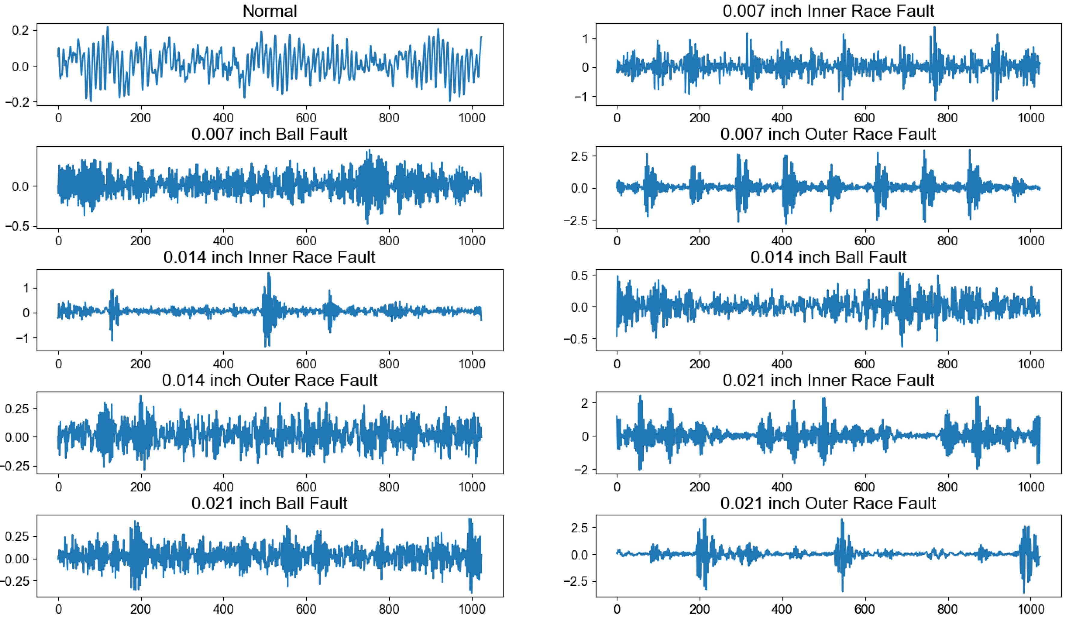
The CWRU dataset used in this study includes vibration signals from ten distinct operational conditions, comprising one normal state and nine different types of bearing faults. The raw time-domain waveforms for these conditions are visualized in Figure 6. Following this, the dataset was partitioned into a training set (8204 samples), a validation set (2344 samples), and a test set (1172 samples) according to a 7:2:1 distribution ratio. All data were preprocessed using the EMDWS framework outlined in Section 3.1 of this study. Figure 7 visually illustrates the signal characteristics before and after preprocessing. As observed, the collaborative processing of EMD and wavelet denoising effectively suppressed noise in the original signal, leading to a substantial improvement in the signal-to-noise ratio of fault features. This enhancement ensures high-quality input for subsequent model training.

Due to the excessive number of IMFs after EMD decomposition, only the visualization graphs of the 0.007-inch inner ring fault before and after EMDWS signal denoising preprocessing are displayed.

4.2.3. Model Performance Evaluation

To ensure optimal model performance, the key hyperparameters of the CNN-Transformer model were tuned using the Bayesian optimization method detailed in Section 3.3. The optimization targeted the accuracy on the validation set, and the resulting optimal hyperparameter configuration after numerous search iterations is listed in

Table 3. Optimal Values after Bayesian Hyperparameter Optimization.

Hyperparameters	Optimized Best Value
batch_size	42
conv1_out	120
conv2_out	159
conv3_out	235
conv4_out	252
dropout_rate	0.131
epochs	21
hidden_dim	69
lr	$5.908\times {10}^{-4}$
num_heads	8
num_layers	2
weight_decay	$5.227\times {10}^{-5}$

.

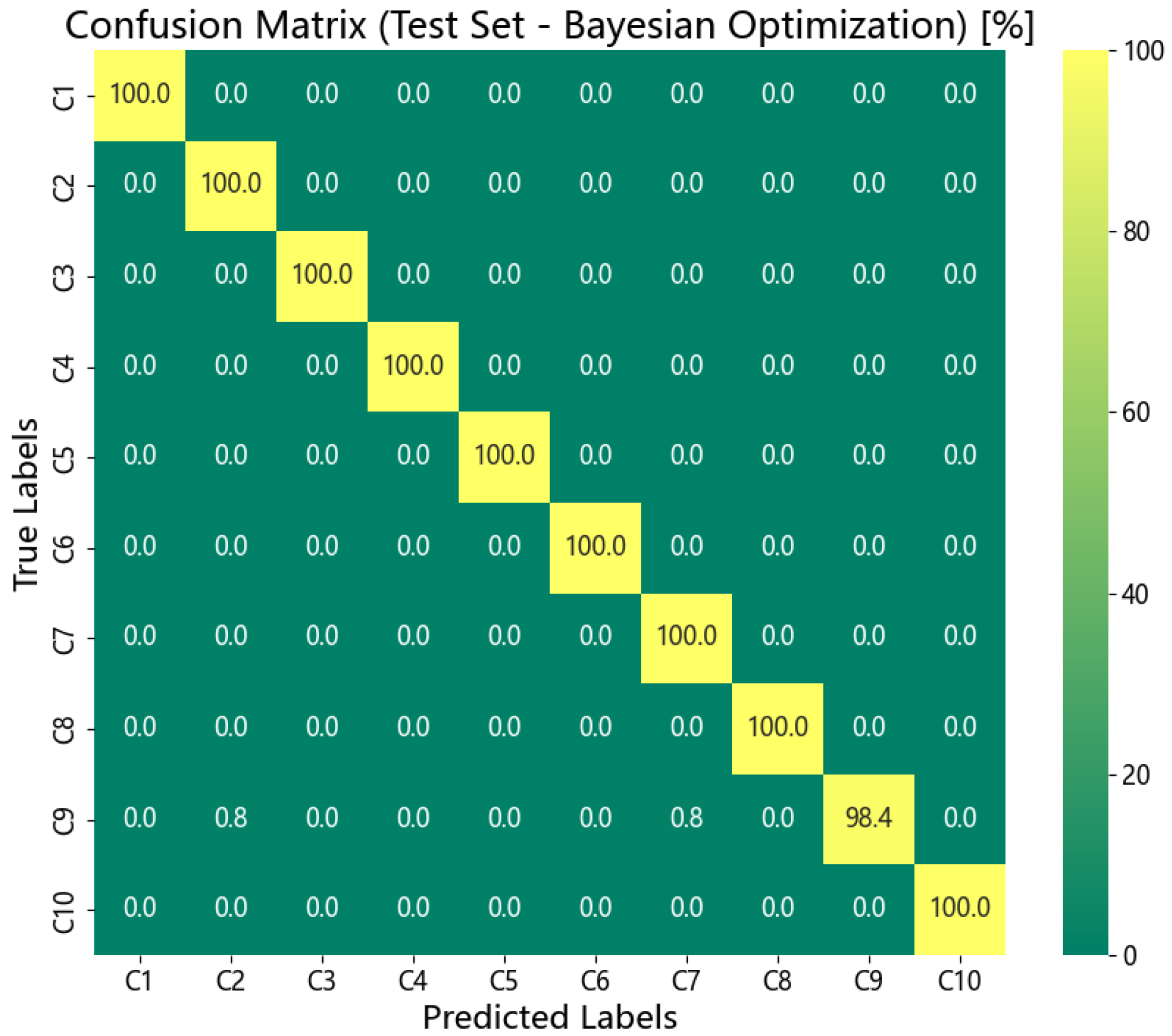
The training process of the model is illustrated in Figure 8, where the curve demonstrates rapid convergence and a stable training process without signs of overfitting. Figure 9 presents the confusion matrix, which further confirms the model’s excellent performance. The model achieves nearly perfect classification across the ten fault types, with only a minimal misclassification rate of 1.6% observed in the “0.007-inch rolling element fault.” This result highlights the effectiveness of the proposed framework.

4.2.4. Ablation and Comparative Experiments

The EMDWS-CNT-BO was compared with three baseline models on the CWRU bearing dataset, and the results are as follows.

Figure 10, Figure 11 and Figure 12 provide a visual representation of the training dynamics and classification outcomes for each baseline model. It is evident from the results that the single-architecture EMD-CNN and EMD-Transformer models exhibit limitations in terms of convergence speed, training stability, and final classification accuracy. Furthermore, their corresponding confusion matrices reveal a higher number of misclassification instances. Although the performance of the initially integrated EMD-CNN-Transformer model shows improvement, the training process still experiences noticeable fluctuations.

Table 4. Comparative Ablation Study Results based on the CWRU Bearing Dataset.

Models	Accuracy (%)	Precision (%)	Recall (%)	F1-Score (%)	Parameters	Inference Time per Sample (ms)
EMD-CNN	96.83 ± 0.26	96.83 ± 0.24	96.86 ± 0.26	96.70 ± 0.23	7562	0.292 ± 0.064
EMD-Transformer	96.67 ± 1.05	96.93 ± 0.89	96.59 ± 1.06	96.61 ± 1.08	110,730	1.261 ± 0.056
EMD-CNN-Transformer	98.58 ± 0.25	98.61 ± 0.24	98.58 ± 0.25	98.58 ± 0.25	286,378	1.274 ± 0.055
EMDWS-CNT-BO	99.85 ± 0.12	99.85 ± 0.11	99.84 ± 0.11	99.84 ± 0.11	595,698	1.806 ± 0.032

summarizes the contribution of each individual component. The baseline hybrid EMD-CNN-Transformer model, with an accuracy of 98.58%, outperforms the standalone EMD-CNN (96.83%) and EMD-Transformer (96.67%) models, thereby confirming the synergistic effect between CNN and Transformer. Furthermore, the complete EMDWS-CNT-BO model achieves a superior accuracy of 99.85%. This significant improvement over the baseline demonstrates that the EMDWS preprocessing module and Bayesian optimization play a critical role in unlocking the full potential of the model. Overall, the experimental results clearly illustrate a progressive enhancement in performance as each functional module is incrementally integrated.

4.2.5. Comparison with Recent Representative Methods

To ensure a more objective and comprehensive evaluation of the proposed EMDWS-CNT-BO framework, we further selected three representative models recently published in high-impact journals for comparative analysis. Following the principles of fairness and reproducibility, we reimplemented these models based on the detailed descriptions provided in their original publications and conducted training and testing under identical experimental conditions as those applied to our framework. The selected models include: the CNN-AM model incorporating an attention mechanism [15]; the advanced SKND-TSACNN framework [3], which integrates a time-scale adaptive CNN (TSACNN) with a neural network denoiser (SKND) through deep fusion; and CLFormer [30], a lightweight Transformer architecture specifically designed for scenarios with limited training samples.

Table 5. Overall performance comparison with representative methods on the CWRU Bearing Dataset.

Models	Accuracy	Precision	Recall	F1-Score	Parameters	Inference Time per Sample (ms)
CNN-AM	98.68 ± 0.33	98.73 ± 0.98	98.46 ± 0.76	98.42 ± 0.87	6282	0.589 ± 0.046
SKND-TSACNN	99.59 ± 0.28	99.63 ± 0.53	99.60 ± 0.53	99.59 ± 0.53	138,190	2.826 ± 0.213
CLFormer	95.78 ± 0.25	95.97 ± 0.68	95.80 ± 0.66	95.58 ± 0.75	8829	2.404 ± 0.145
EMDWS-CNT-BO	99.85 ± 0.12	99.85 ± 0.11	99.84 ± 0.11	99.84 ± 0.11	595,698	1.806 ± 0.032

presents a comprehensive summary of the quantitative performance of all models on the CWRU dataset. As shown in the table, the proposed EMDWS-CNT-BO framework achieves the highest performance across all four core diagnostic metrics: accuracy (99.85%), precision (99.85%), recall (99.84%), and F1 score (99.84%). Regarding model complexity and efficiency, although the proposed framework has the largest parameter count (595,698) due to its systematic architecture, it exhibits superior inference efficiency, with a single-sample inference time of 1.806 ms. This result not only significantly outperforms the structurally complex SKND-TSACNN (2.826 ms), but also surpasses the lightweight CLFormer (2.404 ms), demonstrating an excellent trade-off between performance and efficiency.

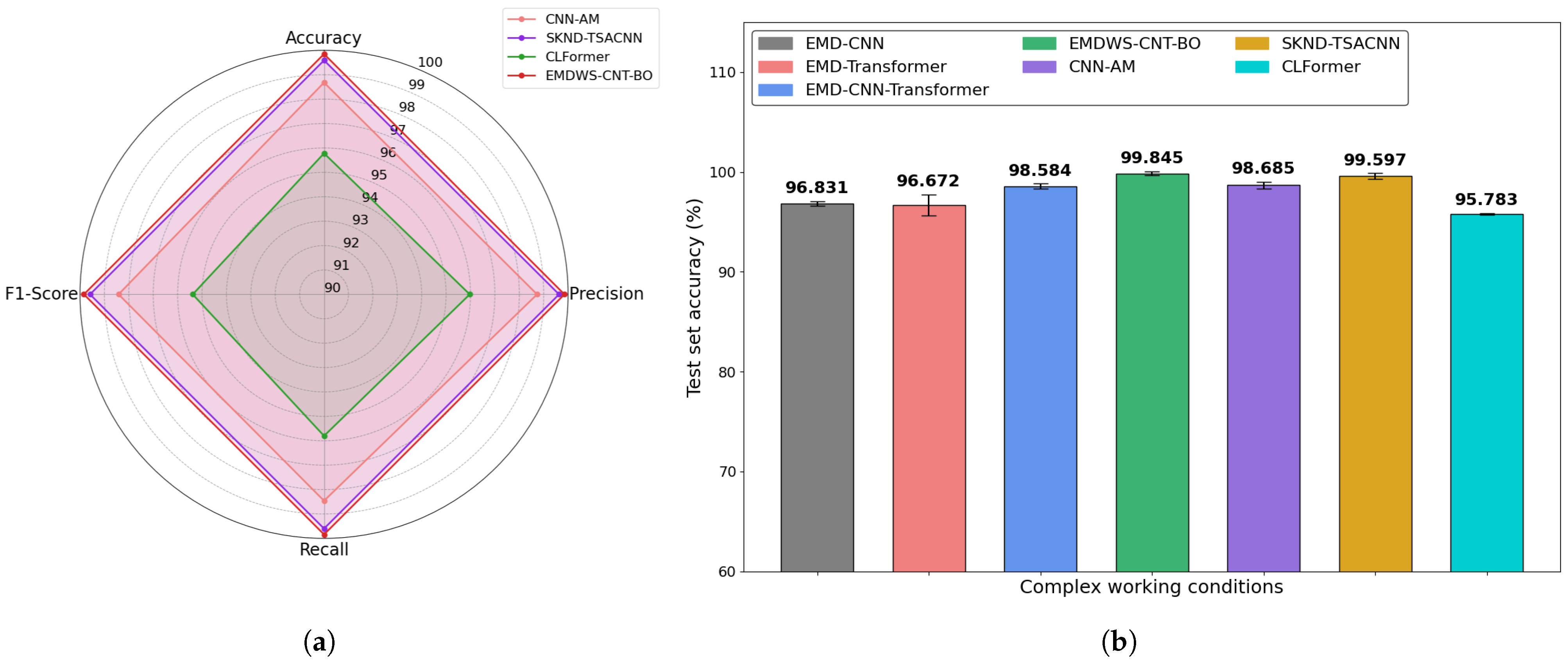
Figure 13 further visualizes these performance differences. The radar chart in Figure 13a clearly shows that our model’s performance envelope has the largest area among all compared methods, proving its superior overall performance across key diagnostic indicators. The bar chart in Figure 13b highlights the robustness advantage of our model, where the error bars represent performance confidence intervals from multiple independent runs. Notably, the EMDWS-CNT-BO model exhibits the narrowest confidence interval (±0.12), providing strong evidence of its enhanced consistency and stability against random data perturbations. Overall, compared to other recent state-of-the-art (SOTA) models, the framework proposed herein achieves an exceptional balance between diagnostic accuracy, model robustness, and inference efficiency.

4.3. Case 2: Simulation Experiment of JNU-Bearing-Dataset

4.3.1. Experimental Platform and Data Settings

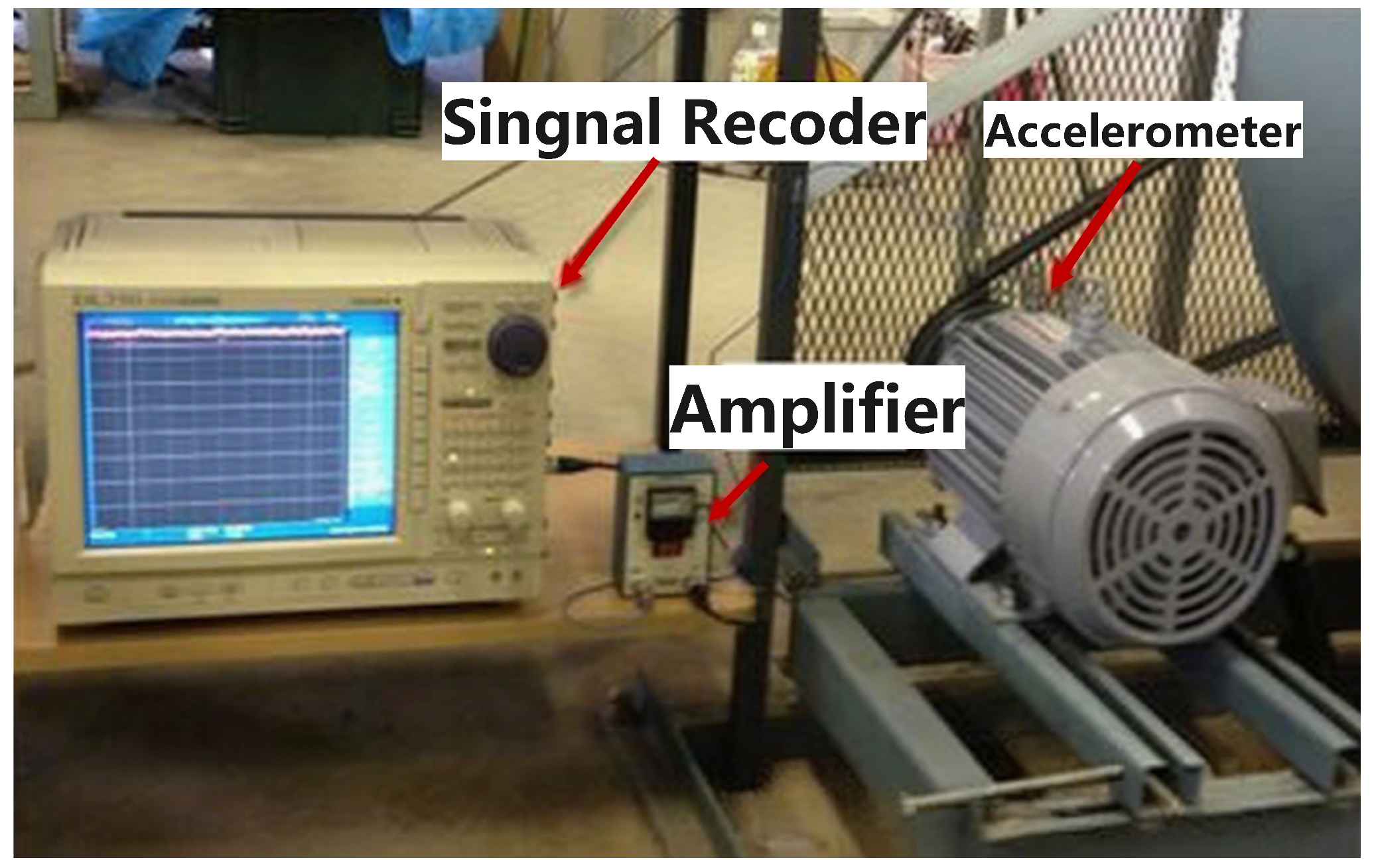
To further validate the generalization capability of the proposed framework across diverse public datasets, the second set of experiments employed the bearing dataset from Jiangnan University (JNU). This dataset was collected from an experimental platform consisting of a centrifugal fan driven by a Mitsubishi SB-JR three-phase induction motor, where vibration signals were acquired using an accelerometer at a sampling frequency of 50 kHz [45,46]. Detailed specifications of the experimental platform are presented in Figure 14.

This experiment focuses on the operational condition at a rotational speed of 800 rpm. The dataset includes four distinct categories: normal condition, inner ring fault, outer ring fault, and rolling element fault. Detailed fault parameters are summarized in

Table 6. Fault Characterization Parameters of the JNU-Bearing-Dataset.

Parameter Category	Specific Item	N205	NU205
Basic Dimensions	Outer diameter	52 mm
	Inner diameter	25 mm
	Width	15 mm
Roller Parameters	Diameter	7 mm
	Quantity	10	11
Contact Angle	Angle	0 rad
Fault Defects (W × D)	Outer race	0.3 × 0.25 mm (Early)	—
	Rolling element	0.5 × 0.15 mm (Early)	—
	Inner race	—	0.3 × 0.35 mm (Early)

. To construct the samples, we applied an overlapping sliding window approach and partitioned the data into a training set (7034 samples), a validation set (2344 samples), and a test set (2346 samples) with a 6:2:2 ratio, enabling a comprehensive evaluation of the model’s diagnostic performance.

4.3.2. Model Performance Evaluation

The EMDWS-CNT-BO model was evaluated on the JNU-Bearing-Dataset, and the optimal hyperparameters derived from the Bayesian optimization algorithm are detailed in the following

Table 7. Optimal Values after Bayesian Hyperparameter Optimization.

Hyperparameters	Optimized Best Value
batch_size	112
conv1_out	60
conv2_out	83
conv3_out	250
conv4_out	239
dropout_rate	0.319
epochs	34
hidden_dim	132
lr	$1.202\times {10}^{-4}$
num_heads	8
num_layers	3
weight_decay	$9.651\times {10}^{-4}$

:

Train the model using this parameter, calculate the loss value and accuracy of the test set, generate the corresponding classification report, and obtain the precision, recall and F1 value of each category in the final fault identification.

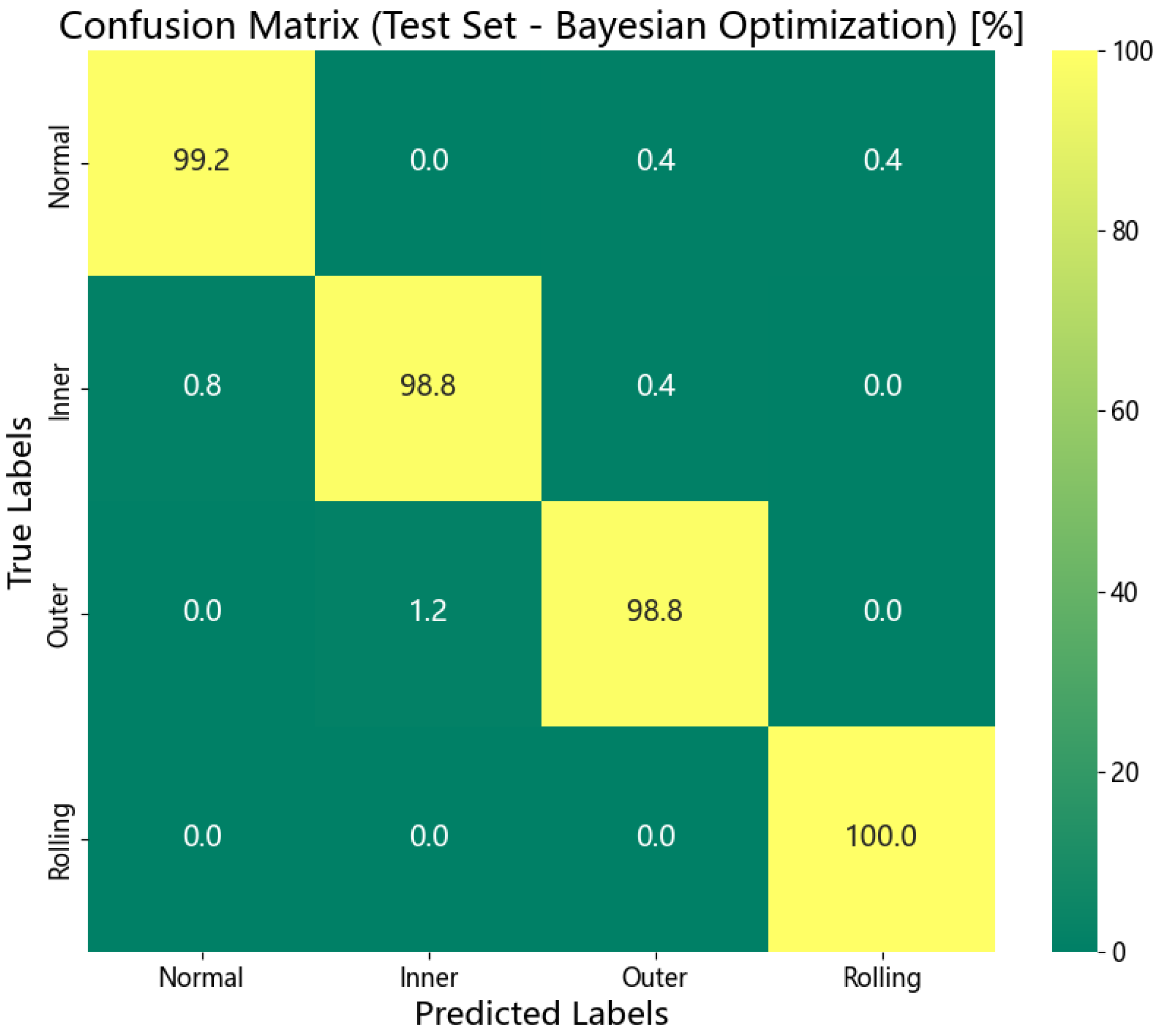
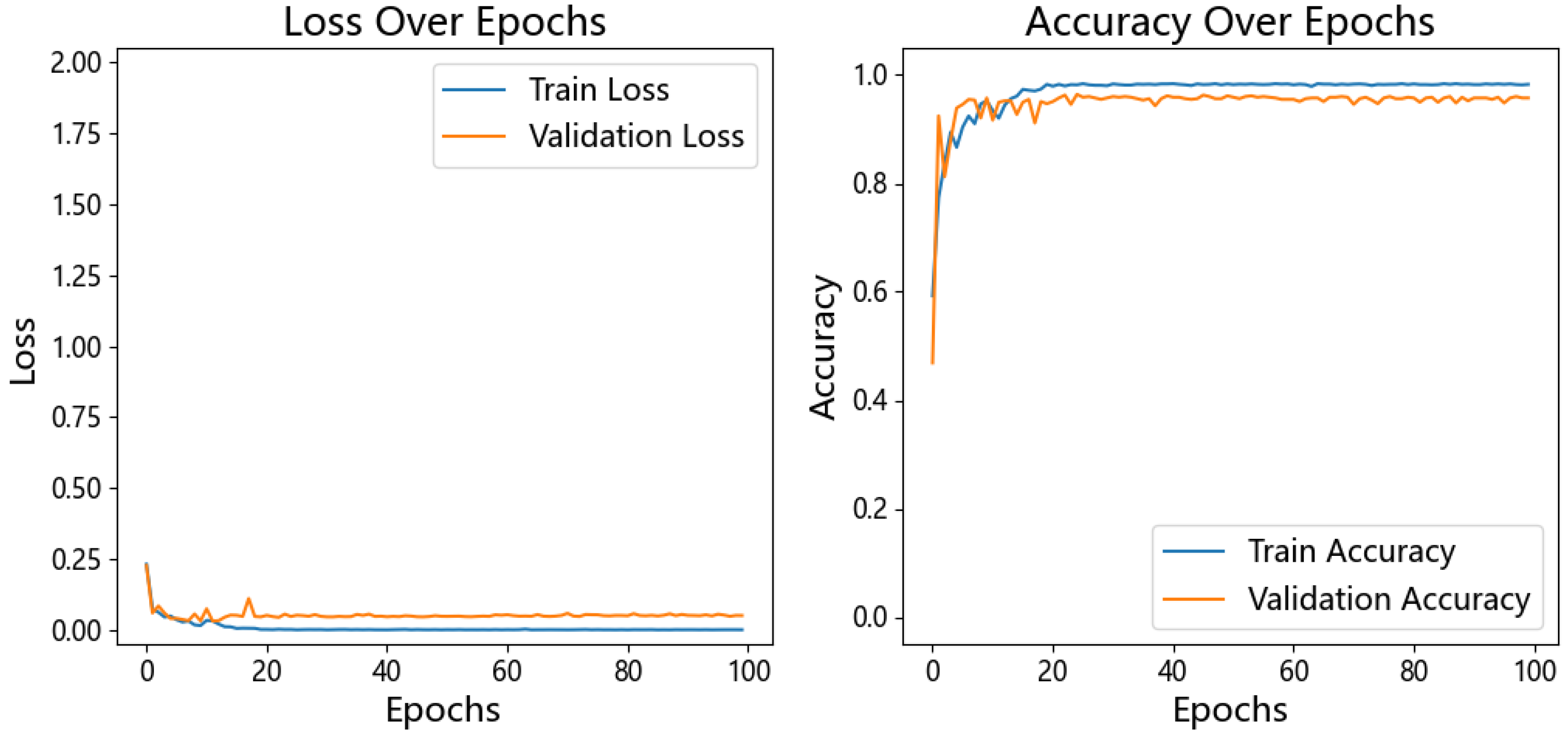
As illustrated in Figure 14 and Figure 15, the model again exhibited excellent performance on this dataset, characterized by a rapid and stable training process as well as an almost perfect confusion matrix (Figure 16), thereby independently validating its effectiveness.

4.3.3. Ablation and Comparative Experiments

The EMDWS-CNT-BO was compared with three baseline models on the JNU-Bearing-Dataset, and the results are as follows.

Figure 17, Figure 18 and Figure 19 provide a visual representation of the training dynamics and final classification performance of the baseline models. As observed from the training curves (Figure 17 and Figure 18), each baseline model demonstrates varying levels of limitations: EMD-CNN exhibits relatively slow convergence; EMD-Transformer shows notable fluctuations in validation loss, indicating instability during training; and although the basic EMD-CNN-Transformer achieves improved performance, a considerable discrepancy remains between its training and validation curves. These observations stand in sharp contrast to the rapid, smooth, and tightly aligned training curves of our proposed model (Figure 15). Furthermore, the confusion matrices in Figure 18 highlight the performance disparities among the baseline models, all of which exhibit significant class confusion, with EMD-Transformer performing the worst in terms of classification accuracy.

Table 8. Comparative Ablation Study Results based on the JNU Bearing Dataset.

Model Name	Accuracy	Precision	Recall	F1-Score	Parameters	Inference Time per Sample (ms)
EMD-CNN	96.44 ± 0.19	96.44 ± 0.24	96.44 ± 0.19	96.43 ± 0.19	7172	0.017 ± 0.003
EMD-Transformer	92.67 ± 0.86	93.04 ± 0.74	92.66 ± 0.86	92.73 ± 0.84	110,388	0.046 ± 0.041
EMD-CNN-Transformer	97.40 ± 0.25	97.40 ± 0.25	96.46 ± 0.25	96.46 ± 0.25	283,300	0.848 ± 0.046
EMDWS-CNT-BO	99.81 ± 0.12	99.81 ± 0.14	99.79 ± 0.15	99.81 ± 0.12	589,548	1.643 ± 0.089

presents a precise quantitative summary of the final performance of all models. The results indicate that the EMDWS-CNT-BO framework proposed in this study achieved a dominant performance advantage, with both an accuracy rate and F1 score reaching 99.81%. The standalone EMD-Transformer model exhibited the lowest accuracy on this dataset, achieving only 92.67%. In contrast, the preliminary fusion model EMD-CNN-Transformer (97.40%) showed improved performance but still lagged significantly behind the proposed framework. This substantial improvement—from 97.40% to 99.81%—clearly demonstrates that the integration of systematic EMDWS preprocessing with Bayesian optimization plays a critical role in unlocking the model’s full potential and enhancing its generalization capability.

4.3.4. Comparison with Recent Representative Methods

To further validate the generalization capability of the EMDWS-CNT-BO framework across diverse datasets, we conducted comparative experiments on the JNU Bearing Dataset.

The quantitative results presented in

Table 9. Overall performance comparison with representative methods on the JNU Bearing Dataset.

Models	Accuracy	Precision	Recall	F1-Score	Parameters	Inference Time per Sample (ms)
CNN-AM	97.97 ± 1.24	98.06 ± 1.06	97.97 ± 1.25	97.98 ± 1.27	6084	0.988 ± 0.032
SKND-TSACNN	99.70 ± 0.20	99.63 ± 0.53	99.60 ± 0.53	99.59 ± 0.53	136,648	3.355 ± 0.426
CLFormer	99.27 ± 0.18	99.25 ± 0.18	99.28 ± 0.18	99.26 ± 0.18	8631	2.484 ± 0.142
EMDWS-CNT-BO	99.81 ± 0.12	99.81 ± 0.14	99.79 ± 0.15	99.81 ± 0.12	589,548	1.643 ± 0.089

further confirm the findings observed on the CWRU dataset. The EMDWS-CNT-BO model proposed in this study continues to outperform other models in critical diagnostic metrics, including an accuracy rate of 99.81% and an F1 score of 99.81%. Moreover, its inference speed (1.643 ms) remains superior to that of comparably complex models such as SKND-TSACNN, highlighting its consistent advantages in both performance and computational efficiency.

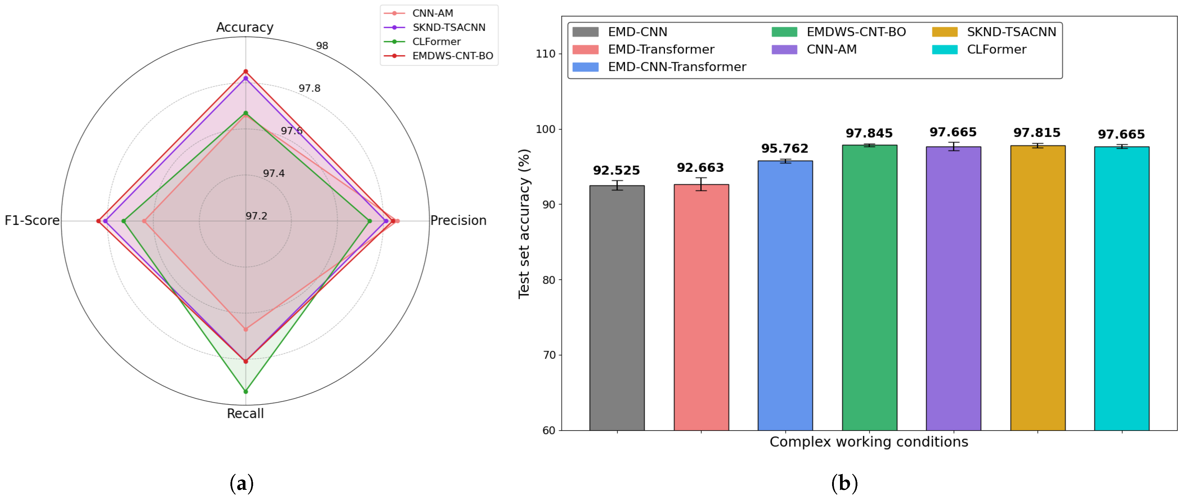
The visual analysis of Figure 20 further underscores the model’s comprehensive performance. Figure 20a presents a radar chart that intuitively illustrates the most complete performance envelope, while Figure 20b employs a bar chart to demonstrate superior stability and robustness across diverse data distributions, as evidenced by the narrowest confidence interval (±0.12) among all models. This consistent cross-dataset performance offers compelling support for the advanced capabilities and broad applicability of our framework.

4.4. Case 3:Simulation Experiment of Self-Built Dataset

4.4.1. Experimental Platform and Data Settings

The rotating machinery fault experimental platform is illustrated in the Figure 21. It is a SSF-DFP-100mini portable mechanical fault demonstration platform. The platform includes six bearing bases, three of which are equipped with bearings featuring inner ring faults, outer ring faults, and ball element faults, while the remaining three are fitted with normal bearings. Specifications of the faulty bearings are as follows: the inner ring fault bearing has a groove defect measuring 0.8 mm in width and 0.3 mm in depth in the inner raceway; the outer ring fault bearing features a groove defect of the same dimensions (0.8 mm * 0.3 mm) in the outer raceway; and the ball fault bearing contains a groove defect measuring 0.8 mm in width, 0.3 mm in depth, and 2 mm in length on the ball surface, as detailed in

Table 10. Fault Types and Corresponding Parameters of the Self-Constructed Bearing Dataset at the Rotor End.

No.	Fault Type	Code	Fault Parameters
1	Normal State	Normal_0	—
2	Rolling Element Fault	ball	0.8 mm × 0.3 mm
3	Inner Ring Fault	inner	0.8 mm × 0.3 mm
4	Outer Ring Fault	outer	0.8 mm × 0.3 mm

.

A single-axis MEMS accelerometer (model SSF-MEMS-X-V1) was mounted at the rotor end—the sensor installation position indicated in Figure 21—to acquire vibration signals at a sampling frequency of 10 kHz. This location is in close proximity to the vibration source, minimizing signal attenuation and enabling the most direct reflection of the bearing’s operational condition. The sensor’s measurement axis is oriented perpendicularly to the radial direction of the rotating shaft and is securely attached to the surface of the bearing housing via a magnetic base, ensuring positional stability throughout the experiment and preventing the introduction of extraneous noise caused by loosening.

This experiment was carried out under no-load conditions (i.e., without external loading). The load acting on the entire rotating system primarily originates from the gravitational force of the rotor and its associated components. The no-load condition was selected to initially evaluate the model’s capability to distinguish various fault types (inner race, outer race, rolling element) under fundamental operating scenarios, while eliminating the potential coupling effects of radial load variations on fault characteristics. This approach allows for a more direct and uncontaminated analysis of vibration differences specifically induced by the faults themselves. The experiment was designed to include four distinct fault categories: one normal condition, one inner race fault, one outer race fault, and one rolling element fault, collectively representing the typical failure modes of critical bearing components. The motor speed was maintained at 2250 r/min to ensure consistent operating conditions. The dataset was specifically constructed to rigorously evaluate the model’s generalization capability. Initially, data were collected in the original experimental environment, sampled using an overlapping sliding window approach, and subsequently randomly partitioned into a training set (2287 samples) and a validation set (762 samples). To simulate real-world variations in working conditions, the test rig was relocated and reinstalled at a new site, where a completely independent dataset was acquired under identical operational parameters. After preprocessing, this dataset constituted a separate test set (764 samples). Prior to each data collection session at both locations, the test rig was operated for approximately 10 min to ensure system stabilization. By physically separating the training/validation data from the test data across different environments, we introduced realistic challenges that better reflect practical scenarios, thereby enabling a more reliable evaluation of the EMDWS-CNT-BO model’s diagnostic accuracy and adaptability under consistent rotational speed and sampling frequency conditions.

4.4.2. Model Performance Evaluation

The EMDWS-CNT-BO model was validated on the self-built dataset, and the optimal parameters obtained by the Bayesian hyperparameter algorithm are shown in the following

Table 11. Optimal Values after Bayesian Hyperparameter Optimization.

Hyperparameters	Optimized Best Value
batch_size	102
conv1_out	62
conv2_out	74
conv3_out	152
conv4_out	230
dropout_rate	0.412
epochs	44
hidden_dim	167
lr	$2.159\times {10}^{-4}$
num_heads	8
num_layers	3
weight_decay	$1.346\times {10}^{-4}$

:

Train the model using this parameter, calculate the loss value and accuracy of the test set, generate the corresponding classification report, and obtain the precision, recall and F1 value of each category in the final fault identification.

As shown in the training monitoring curve (Figure 22), the model’s training process remains highly effective. Both the training and validation losses rapidly decrease and converge to an extremely low and stable level within the first few epochs. Concurrently, the training and validation accuracies quickly reach a near-saturation high-performance level, with the two curves closely aligning throughout the training process. This demonstrates that the model exhibits not only high learning efficiency but also robust generalization performance, with no observable signs of overfitting.

The confusion matrix presented in Figure 23 provides a quantitative evaluation of the model’s final classification performance on the test set. The matrix exhibits a distinct diagonal pattern, demonstrating that the model achieves exceptionally high recognition accuracy across the majority of fault categories. Specifically, the recognition rates for “Normal” and “Inner” faults reach 100% and 99.5%, respectively. At the same time, the matrix objectively reveals the model’s confusion areas, which are primarily observed between “Outer” and “Rolling” faults, where approximately 12.7% of “Outer” faults are misclassified as “Rolling” faults. Despite this limited degree of misclassification, the model’s overall diagnostic performance remains highly robust.

4.4.3. Ablation and Comparative Experiments

The EMDWS-CNT-BO was compared with three baseline models on the Self-built Bearing Dataset, and the results are as follows:

The training and validation curves, presented in Figure 24 and Figure 25, clearly demonstrate that the baseline models generally suffer from limited generalization capabilities. The EMD-CNN model exhibits a pronounced overfitting tendency in the later stages of training, whereas the EMD-Transformer displays an unstable training process characterized by significant fluctuations. Furthermore, the confusion matrices, shown in Figure 26, reveal notable deficiencies in their classification performance. Specifically, all baseline models consistently struggle to distinguish between the “outer ring fault” and “rolling element fault” categories, resulting in substantial misclassification between these two fault types.

As shown in

Table 12. Comparative Ablation Study Results based on the Self-built Bearing Dataset.

Model Name	Accuracy	Precision	Recall	F1-Score	Parameters	Inference Time per Sample (ms)
EMD-CNN	92.53 ± 0.63	92.68 ± 0.49	93.15 ± 0.53	93.10 ± 0.57	7172	0.024 ± 0.011
EMD-Transformer	92.66 ± 0.86	93.04 ± 0.74	92.66 ± 0.86	92.73 ± 0.84	110,388	0.056 ± 0.023
EMD-CNN-Transformer	95.76 ± 0.15	95.95 ± 0.21	95.89 ± 0.12	95.89 ± 0.13	283,300	0.921 ± 0.423
EMDWS-CNT-BO	97.85 ± 0.09	97.84 ± 0.12	97.81 ± 0.11	97.84 ± 0.09	589,548	1.401 ± 0.644

, the performance of the single-architecture models EMD-CNN (92.53% accuracy) and EMD-Transformer (92.66% accuracy) is relatively limited. The basic hybrid architecture, EMD-CNN-Transformer, increases the accuracy to 95.76%, thereby demonstrating the initial effectiveness of combining different architectural components. However, it is only our complete EMDWS-CNT-BO framework that achieves a significantly higher accuracy of 97.85% under the same challenging conditions. This substantial improvement—from 95.76% to 97.85%—provides compelling evidence that systematic EMDWS preprocessing, together with Bayesian optimization, plays a critical role in mitigating overfitting and enhancing both the robustness and generalization capability of the model when confronted with real-world domain shift scenarios.

4.4.4. Comparison with Recent Representative Methods

To evaluate the model’s robustness under conditions that closely simulate real-world industrial environments, we conducted experiments on a self-constructed dataset in the final stage of our study.

As presented in

Table 13. Overall performance comparison with representative methods on the Self-Constructed Dataset.

Models	Accuracy	Precision	Recall	F1-Score	Parameters	Inference Time per Sample (ms)
CNN-AM	97.66 ± 0.55	97.86 ± 0.98	97.67 ± 1.11	97.64 ± 1.13	6084	0.843 ± 0.027
SKND-TSACNN	97.82 ± 0.31	97.81 ± 0.33	97.81 ± 0.32	97.81 ± 0.32	136,648	2.862 ± 0.363
CLFormer	97.67 ± 0.27	97.74 ± 0.67	97.94 ± 0.56	97.73 ± 0.72	8631	2.119 ± 0.121
EMDWS-CNT-BO	97.85 ± 0.09	97.84 ± 0.12	97.81 ± 0.11	97.84 ± 0.09	589,548	1.401 ± 0.644

, the quantitative results confirm that, as anticipated, the cross-environment configuration resulted in a performance degradation across all models. Nevertheless, even under these most demanding conditions, the proposed EMDWS-CNT-BO framework maintained superior performance, achieving the highest accuracy (97.85%) and F1 score (97.84%). Moreover, its inference efficiency (1.401 ms) consistently surpassed that of other complex models, further validating its effective balance between high performance and computational efficiency.

As illustrated in Figure 27a,b, the visualization charts reveal a more comprehensive performance profile. The radar chart in Figure 27a indicates that while our model achieves the best overall balance in F1 score, it exhibits slightly lower performance in individual precision and recall compared to models specifically optimized for those metrics. Nevertheless, the bar chart in Figure 27b emphasizes our model’s most critical advantage: its performance confidence interval (±0.09) remains the narrowest across all models. This provides irrefutable evidence that our model demonstrates the highest consistency and robustness when confronted with real-world distribution shifts. Consequently, although the numerical results show a slight decline in this experiment, they offer a more realistic and meaningful evaluation of the generalization capability of our framework.

5. Discussion

The EMDWS-CNT-BO framework proposed in this study, through its deep integration of systematic signal preprocessing, a hybrid CNN-Transformer architecture, and Bayesian hyperparameter optimization, has demonstrated its superiority as an advanced diagnostic paradigm across multiple bearing datasets. The framework not only achieved near-perfect recognition accuracy on standard datasets but also showcased its robust capability in handling non-stationary, noisy, and imbalanced data.

However, despite the significant success of our framework, we must objectively acknowledge its limitations in the context of complex industrial applications. First, this study validates the model’s effectiveness in a closed-set recognition scenario. A closed-set assumption posits that a test sample must belong to one of the classes known during training. This setup is common in many early simulation-driven AI diagnostic studies, such as the work by Xiang & Zhong [47], who utilized FEM simulation data to train an SVM model for distinguishing several known shaft system faults. While this approach is valuable for validating diagnostic logic and analyzing fault mechanisms, it carries a risk of misclassification in real-world industrial settings, where novel or compound faults not seen during training may emerge at any time.

Second, this challenge is preliminarily highlighted in the custom-built dataset from Case Study 3. By introducing a more realistic domain shift through a change in the experimental venue, the model’s performance, while still high, exhibited a slight degradation compared to its performance on stable datasets. This indicates that subtle variations in data distribution, caused by factors such as background noise and minor adjustments in sensor placement, still pose a challenge to the model’s generalization ability.

Therefore, future work will primarily focus on overcoming the aforementioned limitations. A core direction is to upgrade the model from a closed-set framework to an open-set recognition (OSR) paradigm, endowing it with the ability to identify “unknown” faults and thus avoid forced misclassification. Concurrently, research into model lightweighting and edge deployment is crucial. This involves employing techniques like knowledge distillation and network pruning to maintain high diagnostic accuracy while meeting the real-time monitoring demands of practical equipment such as machine tools. Furthermore, we will continue to optimize the model architecture and incorporate techniques like domain adaptation to enhance its generalization capabilities across different operating conditions and address the challenge of domain shift. Finally, to verify the versatility of our framework, we plan to apply it to a broader range of industrial time-series tasks, such as gearbox fault diagnosis and rotor crack detection, to explore its potential as a general-purpose time-series analysis paradigm.

6. Conclusions

In this work, a significant contribution is made by presenting EMDWS-CNT-BO, a novel and systematic framework for bearing fault diagnosis. The core innovation of this framework lies not in the invention of new standalone components, but in their synergistic and holistic integration to address the complex, multi-faceted challenges of real-world industrial environments. The EMDWS preprocessing pipeline effectively mitigates noise interference and resolves data imbalance, supplying the subsequent deep learning model with high-quality, balanced training data. Furthermore, the integration of a CNN-Transformer model with Bayesian Optimization achieves a sophisticated balance between local feature extraction and global dependency modeling. Our work empirically demonstrates that it is this systematic combination that unlocks superior performance, rather than the simple application of individual techniques.

Validation on three distinct datasets confirms the framework’s superiority. The EMDWS-CNT-BO consistently and significantly surpasses other diagnostic approaches, particularly under fluctuating and noisy conditions. Looking ahead, promising research directions include extending the framework’s application to a broader spectrum of rotating machinery faults. Furthermore, investigations into model lightweighting will be pursued to enable efficient deployment on industrial edge computing platforms.

References

1. Wang, D.; Li, Y.; Jia, L.; Song, Y.; Liu, Y. Novel three-stage feature fusion method of multimodal data for bearing fault diagnosis. IEEE Trans. Instrum. Meas. 2021, 70, 1–10. [Google Scholar] [CrossRef]
2. Lee, C.-Y.; Le, T.-A.; Lin, Y.-T. A feature selection approach hybrid grey wolf and heap-based optimizer applied in bearing fault diagnosis. IEEE Access 2022, 10, 56691–56705. [Google Scholar] [CrossRef]
3. Yu, Z.; Zhang, C.; Liu, J.; Deng, C. SKND-TSACNN: A novel time-scale adaptive CNN framework for fault diagnosis of rotating machinery. Knowl.-Based Syst. 2023, 275, 110682. [Google Scholar] [CrossRef]
4. Zhang, Z.; Huang, W.; Liao, Y.; Song, Z.; Shi, J.; Jiang, X.; Shen, C.; Zhu, Z. Bearing fault diagnosis via generalized logarithm sparse regularization. Mech. Syst. Signal Process. 2022, 167, 108576. [Google Scholar] [CrossRef]
5. Yu, M.; Zhang, Y.; Yang, C. Rolling bearing faults identification based on multiscale singular value. Adv. Eng. Inform. 2023, 57, 102040. [Google Scholar] [CrossRef]
6. Li, Z.; Liu, N.; Zhang, X.; Luo, Y. Research on Fault Diagnosis of Rotating Machinery Based on Improved Convolutional Neural Network. J. Liaoning Inst. Sci. Technol. 2025, 27, 24–29. [Google Scholar]
7. Gao, S.; Li, T.; Zhang, Y.; Pei, Z. Fault diagnosis method of rolling bearings based on adaptive modified CEEMD and 1DCNN model. ISA Trans. 2023, 140, 309–330. [Google Scholar] [CrossRef] [PubMed]
8. Li, H.; Wang, T.; Zhang, F.; Chu, F. KurVMDPgram: A Signal Decomposition Algorithm for Fault Diagnosis of Rotating Machinery. J. Mech. Eng. 2025, 61, 11–23. [Google Scholar]
9. Li, J.; Wang, H.; Wang, X.; Zhang, Y. Rolling bearing fault diagnosis based on improved adaptive parameterless empirical wavelet transform and sparse denoising. Measurement 2020, 152, 107392. [Google Scholar] [CrossRef]
10. Dong, H.; Zheng, K.; Wen, S.; Zhang, Z.; Li, Y.; Zhu, B. Lightweight Ghost Enhanced Feature Attention Network: An Efficient Intelligent Fault Diagnosis Method under Various Working Conditions. Sensors 2024, 24, 3691. [Google Scholar] [CrossRef]
11. Zhang, K.; Fan, C.; Zhang, X.; Shi, H.; Li, S. A hybrid deep-learning model for fault diagnosis of rolling bearings in strong noise environments. Meas. Sci. Technol. 2022, 33, 065103. [Google Scholar] [CrossRef]
12. Geng, D.; Tong, H. Optimized Analysis of Mechanical Vibration Signals Through Improved Wavelet Threshold Denoising. In Proceedings of the 2024 6th International Symposium on Robotics & Intelligent Manufacturing Technology (ISRIMT), Shanghai, China, 24–26 May 2024; pp. 187–191. [Google Scholar]
13. Li, H.; Shi, J.; Li, L.; Tuo, X.; Qu, K.; Rong, W. Novel wavelet threshold denoising method to highlight the first break of noisy microseismic recordings. IEEE Trans. Geosci. Remote Sens. 2022, 60, 1–10. [Google Scholar] [CrossRef]
14. Hao, W.; Liu, F. Imbalanced data fault diagnosis based on an evolutionary online sequential extreme learning machine. Symmetry 2020, 12, 1204. [Google Scholar] [CrossRef]
15. Wang, Z.; Liu, T.; Wu, X.; Liu, C. A diagnosis method for imbalanced bearing data based on improved SMOTE model combined with CNN-AM. J. Comput. Des. Eng. 2023, 10, 1930–1940. [Google Scholar] [CrossRef]
16. Yang, D.; Karimi, H.R.; Gelman, L. An explainable intelligence fault diagnosis framework for rotating machinery. Neurocomputing 2023, 541, 126257. [Google Scholar] [CrossRef]
17. Zhong, W.; Jiang, J.; Song, Y.; Zhang, L.; Gu, Q. A Prediction Model for the Remaining Useful Life of Rolling Bearings Based on Improved CNN-BGRU. J. Mech. Electr. Eng. 2025, 12, 1–12. [Google Scholar]
18. Wang, X.; Hua, T.; Xu, S.; Zhao, X. A novel rolling bearing fault diagnosis method based on BLS and CNN with attention mechanism. Machines 2023, 11, 279. [Google Scholar] [CrossRef]
19. Ma, N.; Sun, L.; He, Y.; Zhou, C.; Dong, C. CNN-TransNet: A hybrid CNN-transformer network with differential feature enhancement for cloud detection. IEEE Geosci. Remote Sens. Lett. 2023, 20, 1–5. [Google Scholar] [CrossRef]
20. He, Z.; Fu, G.; Cao, Y.; Cao, Y.; Yang, J.; Li, X. ESKN: Enhanced selective kernel network for single image super-resolution. Signal Process. 2021, 189, 108274. [Google Scholar] [CrossRef]
21. Ni, J.; Shen, K.; Chen, Y.; Cao, W.; Yang, S.X. An improved deep network-based scene classification method for self-driving cars. IEEE Trans. Instrum. Meas. 2022, 71, 1–14. [Google Scholar] [CrossRef]
22. Chen, Z.; Chen, J.; Liu, S.; Feng, Y.; He, S.; Xu, E. Multi-channel calibrated transformer with shifted windows for few-shot fault diagnosis under sharp speed variation. ISA Trans. 2022, 131, 501–515. [Google Scholar] [CrossRef]
23. Liang, P.; Yu, Z.; Wang, B.; Xu, X.; Tian, J. Fault transfer diagnosis of rolling bearings across multiple working conditions via subdomain adaptation and improved vision transformer network. Adv. Eng. Inform. 2023, 57, 102075. [Google Scholar] [CrossRef]
24. Yang, L.; Jiang, X.; Li, X.; Zhu, Z. Self-supervised learning with signal masking and reconstruction for machinery fault diagnosis under limited labeled data and varying working condition. IEEE Sens. J. 2023, 23, 24862–24873. [Google Scholar] [CrossRef]
25. Zhu, S.; Liao, B.; Hua, Y.; Zhang, C.; Wan, F.; Qing, X. A transformer model with enhanced feature learning and its application in rotating machinery diagnosis. ISA Trans. 2023, 133, 1–12. [Google Scholar] [CrossRef] [PubMed]
26. Li, Y.; Zhou, Z.; Sun, C.; Chen, X.; Yan, R. Variational attention-based interpretable transformer network for rotary machine fault diagnosis. IEEE Trans. Neural Netw. Learn. Syst. 2022, 35, 6180–6193. [Google Scholar] [CrossRef]
27. Chen, J.; Yue, J.; Chen, Y.; Zhou, H.; Hu, Z. Nonlinear activation functions are not necessary: A lightweight nonlinear activation free network based on multi-scale large kernel attention mechanism for fault diagnosis. IEEE Sens. J. 2025, 25, 18926–18940. [Google Scholar] [CrossRef]
28. Wang, J.; Shao, H.; Yan, S.; Liu, B. C-ECAFormer: A new lightweight fault diagnosis framework towards heavy noise and small samples. Eng. Appl. Artif. Intell. 2023, 126, 107031. [Google Scholar] [CrossRef]
29. Han, Y.; Zhang, F.; Li, Z.; Wang, Q.; Li, C.; Lai, P.; Li, T.; Teng, F.; Jin, Z. Mt-ConvFormer: A multi-task bearing fault diagnosis method using a combination of CNN and transformer. IEEE Trans. Instrum. Meas. 2024, 74, 3501816. [Google Scholar] [CrossRef]
30. Fang, H.; Deng, J.; Bai, Y.; Feng, B.; Li, S.; Shao, S.; Chen, D. CLFormer: A lightweight transformer based on convolutional embedding and linear self-attention with strong robustness for bearing fault diagnosis under limited sample conditions. IEEE Trans. Instrum. Meas. 2021, 71, 1–8. [Google Scholar] [CrossRef]
31. Lu, Y.; Wang, Z.; Xie, R.; Zhang, J.; Pan, Z.; Liang, S.Y. Bayesian optimized deep convolutional network for bearing diagnosis. Int. J. Adv. Manuf. Technol. 2020, 108, 313–322. [Google Scholar] [CrossRef]
32. Fan, H.; Shao, S.; Zhang, X.; Wan, X.; Cao, X.; Ma, H. Intelligent fault diagnosis of rolling bearing using FCM clustering of EMD-PWVD vibration images. IEEE Access 2020, 8, 145194–145206. [Google Scholar] [CrossRef]
33. Yin, C.; Wang, Y.; Ma, G.; Wang, Y.; Sun, Y.; He, Y. Weak fault feature extraction of rolling bearings based on improved ensemble noise-reconstructed EMD and adaptive threshold denoising. Mech. Syst. Signal Process. 2022, 171, 108834. [Google Scholar] [CrossRef]
34. Yuan, J.; Xu, C.; Zhao, Q.; Jiang, H.; Weng, Y. High-fidelity noise-reconstructed empirical mode decomposition for mechanical multiple and weak fault extractions. ISA Trans. 2022, 129, 380–397. [Google Scholar] [CrossRef]
35. Jiao, Z.; Yang, T.; Gao, X.; Chen, S.; Liu, W. Welding penetration monitoring for ship robotic GMAW using arc sound sensing based on improved wavelet denoising. Machines 2023, 11, 911. [Google Scholar] [CrossRef]
36. Lei, C.; Jiao, M.; Fan, G.; Liu, S.; Xue, L.; Li, J. Rolling Bearing Fault Diagnosis Method Based on SSA-IWT-EMD. J. Beijing Univ. Aeronaut. Astronaut. 2025, 51, 1152–1162. [Google Scholar]
37. Zhang, J.; Hu, M.; Huang, F. Flight Normal Rate Prediction Based on SMOTE Algorithm. J. East China Jiaotong Univ. 2025, 42, 57–66. [Google Scholar]
38. Saputra, D.C.E.; Sunat, K.; Ratnaningsih, T. SMOTE-MRS: A Novel SMOTE-Multiresolution Sampling technique for imbalanced distribution to improve prediction of anemia. IEEE Access 2024, 12, 1204. [Google Scholar]
39. Santry, D.J. Convolutional Neural Networks. In Demystifying Deep Learning: An Introduction to the Mathematics of Neural Networks; IEEE: Piscataway, NJ, USA, 2024; pp. 111–131. [Google Scholar]
40. Fu, W.; Li, S.; Zheng, B.; Zhu, X.; Xiong, H.; Shao, M. Rolling Bearing Fault Diagnosis Based on Multi-scale Residual Attention Network and Adaptive Transformer Encoder. Mach. Tool Hydraul. 2025, 53, 1–9. [Google Scholar]
41. Frazier, P.I. A tutorial on Bayesian optimization. arXiv 2018, arXiv:1807.02811. [Google Scholar] [CrossRef]
42. Sasaki, T.; Bandoh, Y.; Kitahara, M. Complexity Reduction of Graph Signal Denoising Based on Fast Graph Fourier Transform. In Proceedings of the 2023 IEEE International Conference on Image Processing (ICIP), Kuala Lumpur, Malaysia, 8–11 October 2023; pp. 1910–1914. [Google Scholar]
43. Smith, W.A.; Randall, R.B. Rolling element bearing diagnostics using the Case Western Reserve University data: A benchmark study. Mech. Syst. Signal Process. 2015, 64, 100–131. [Google Scholar] [CrossRef]
44. Zhou, X.; Yang, Z.; Wu, W. Rotating Machinery Fault Diagnosis Based on Multi-channel Parallel LSTM-CNN. Ind. Instrum. Autom. Devices 2025, 2, 92–98. [Google Scholar]
45. Zhao, Z.; Li, T.; Wu, J.; Sun, C.; Wang, S.; Yan, R.; Chen, X. Deep learning algorithms for rotating machinery intelligent diagnosis: An open source benchmark study. ISA Trans. 2020, 107, 224–255. [Google Scholar] [CrossRef] [PubMed]
46. Xie, Y.; Zhang, J. A Small Sample Fault Diagnosis Method for Bearings and Gears Based on Triplet Network. J. Mech. Electr. Eng. 2022, 39, 8. [Google Scholar]
47. Xiang, J.; Zhong, Y. A Novel Personalized Diagnosis Methodology Using Numerical Simulation and an Intelligent Method to Detect Faults in a Shaft. Appl. Sci. 2016, 6, 414. [Google Scholar] [CrossRef]
Figure 1. Convolutional Neural Network (CNN) architecture.
Machines 13 00865 g001
Figure 3. Model Architecture Flowchart.
Machines 13 00865 g003
Figure 5. Rolling bearing experimental platform.
Machines 13 00865 g005
Figure 6. Visualized vibration signals of ten types of faults.
Machines 13 00865 g006
Figure 7. Visualized graphs of the signal before and after denoising preprocessing by EMDWS.
Machines 13 00865 g007
Figure 8. Training Monitoring Curve of EMDWS-CNT-BO.
Machines 13 00865 g008
Figure 9. Confusion Matrix of EMDWS-CNT-BO.
Machines 13 00865 g009
Figure 10. Loss for each epochs of different models: (a) EMD-CNN; (b) EMD-Transformer; (c) EMD-CNN-Transformer.
Machines 13 00865 g010
Figure 11. Accuracy for each epochs of different models: (a) EMD-CNN; (b) EMD-Transformer; (c) EMD-CNN-Transformer.
Machines 13 00865 g011
Figure 12. Confusion matrix for each epochs of different models: (a) EMD-CNN; (b) EMD-Transformer; (c) EMD-CNN-Transformer.
Machines 13 00865 g012
Figure 13. Visual performance comparison with representative methods on the CWRU Bearing Dataset: (a) Radar chart comparing key diagnostic metrics; (b) Bar chart of average test set accuracy with confidence intervals.
Machines 13 00865 g013
Figure 14. Mitsubishi SB-JR Induction Motor Fault Diagnosis Test Rig.
Machines 13 00865 g014
Figure 15. Training Monitoring Curve of EMDWS-CNT-BO.
Machines 13 00865 g015
Figure 16. Confusion Matrix of EMDWS-CNT-BO.
Machines 13 00865 g016
Figure 17. Loss for each epochs of different models: (a) EMD-CNN; (b) EMD-Transformer; (c) EMD-CNN-Transformer.
Machines 13 00865 g017
Figure 18. Accuracy for each epochs of different models: (a) EMD-CNN; (b) EMD-Transformer; (c) EMD-CNN-Transformer.
Machines 13 00865 g018
Figure 19. Confusion matrix for each epochs of different models: (a) EMD-CNN; (b) EMD-Transformer; (c) EMD-CNN-Transformer.
Machines 13 00865 g019
Figure 20. Visual performance comparison with representative methods on the JNU Bearing Dataset: (a) Radar chart comparing key diagnostic metrics; (b) Bar chart of average test set accuracy with confidence intervals.
Machines 13 00865 g020
Figure 21. Self-Constructed Bearing Dataset Experimental Platform.
Machines 13 00865 g021
Figure 22. Training Monitoring Curve of EMDWS-CNT-BO.
Machines 13 00865 g022
Figure 23. Confusion Matrix of EMDWS-CNT-BO.
Machines 13 00865 g023
Figure 24. Loss for each epochs of different models: (a) EMD-CNN; (b) EMD-Transformer; (c) EMD-CNN-Transformer.
Machines 13 00865 g024
Figure 25. Accuracy for each epochs of different models: (a) EMD-CNN; (b) EMD-Transformer; (c) EMD-CNN-Transformer.
Machines 13 00865 g025
Figure 26. Confusion matrix for each epochs of different models: (a) EMD-CNN; (b) EMD-Transformer; (c) EMD-CNN-Transformer.
Machines 13 00865 g026
Figure 27. Visual performance comparison with representative methods on the Self-Constructed Bearing Dataset: (a) Radar chart comparing key diagnostic metrics; (b) Bar chart of average test set accuracy with confidence intervals.
Machines 13 00865 g027