Abstract
The increasing number of space exploration missions and the complexity of exploration missions have brought great challenges to the design of launch vehicles. The guidance system is the key subsystem of launch vehicles and the key to the success of launch. Traditional document-based design patterns have been increasingly unable to cope with the problems of insufficient expression, rapid change analysis, and design iteration brought by the increase in system complexity. Employing the MBSE (Model-Based Systems Engineering) method in guidance system design has the advantages of integrated design, closed-loop verification, and fast iteration. The co-simulation between the system-level MBSE model—which captures requirements, functions, and architecture—and domain model (e.g., CAD models and MATLAB-based guidance algorithms, representing discipline-specific implementation models) is conducive to verification and accurate trade-off analysis under frequent changes in requirements and provides support for the rapid design and selection of the launch vehicle guidance system.
1. Introduction
The growing frequency of space exploration missions and their increasing operational complexity present significant challenges to launch vehicle design. As the core operational framework of rocket systems, the Guidance, Navigation, and Control (GNC) system plays a critical role in maintaining precise trajectory adherence and ensuring seamless transition between flight phases [1,2]. This integrated system comprises three functional components: the navigation subsystem responsible for measuring and calculating vehicle motion parameters, the guidance subsystem that generates operational commands, and the control subsystem that executes these commands to maintain flight stability against launch disturbances.
Optimal design of navigation and guidance systems constitutes a fundamental prerequisite for successful rocket launches [3]. Inadequate system design specifications or incomplete verification of those specifications can directly compromise orbital insertion accuracy and, in the worst case, lead to mission failure. These challenges are exacerbated by escalating system complexity and evolving stakeholder requirements, which conventional design methodologies increasingly fail to address in sophisticated navigation and guidance applications.
Traditional aerospace engineering practices predominantly employ document-centric design approaches using natural language specifications. However, as system complexity intensifies, this method reveals critical limitations including expression ambiguity, specification inconsistency across documentation versions, and difficulties in conducting comprehensive change impact analyses and simulation validations—all of which impede rapid system development and iterative optimization [4,5,6].
Model-Based Systems Engineering (MBSE) [7,8,9] has emerged as a transformative methodology, formally defined as “the formalized application of modeling to support system requirements design, analysis, verification, and validation activities throughout the system lifecycle from conceptual design to post-development phases.” MBSE addresses complex system modeling challenges through tripartite analysis of requirements, architecture, and behavior, enabling comprehensive system requirement analysis and behavioral verification [4,10,11].
The engineering community has increasingly adopted MBSE methodologies due to their demonstrated advantages in design optimization [12,13], closed-loop verification capabilities [14,15], cost-effectiveness [16], and rapid iteration potential [17,18]. Recent applications span multiple domains including, as an example, using MBSE and the DoDAF (Department of Defense Architecture Framework) to improve the design of manned lunar landing systems. Through SysML modeling and logical simulation verification, the challenges of information traceability and requirement management in traditional text mode are solved [19]. The method of structured modeling and multi-perspective requirement analysis is proposed and used to improve the process of aeronautical equipment support and civil aircraft design [20,21]. Ref. [22] introduced a method based on airworthiness compliance evidence chains for planning and designing certification flight test scenarios for civil aircraft. Additionally, Ref. [23] addressed the characteristics of the current civil aircraft development process and proposed a process management method based on MBSE. The MBSE modeling approach was also utilized to construct digital twin systems for industrial robots [24] and to develop multi-stage weapon target allocation strategies [25].
Extensive scholarly efforts have been devoted to rocket system research, with notable advancements in model-based methodologies. As documented in Ref. [12], comprehensive investigations into launch vehicle architecture resulted in the development of an innovative model-based framework for integrated system design. This pioneering work addressed critical challenges in system development through systematic modeling solutions. Subsequent studies further expanded these methodologies: ref. [26] implemented MBSE principles to simulate stage separation dynamics between primary and secondary rocket components, establishing rigorous requirement specifications through multi-level architectural modeling encompassing operational requirements, logical frameworks, and physical implementations. Complementary research by ref. [27] demonstrated the efficacy of Modelica language in validating complex aerospace power system architectures. Meanwhile, ref. [28] pioneered the application of model-view approaches for concurrent evaluation of manufacturing tooling configurations and failure mode effects in sounding rocket design. Despite these advancements, the current literature reveals a significant research gap in applying MBSE methodologies, specifically to rocket guidance system optimization, and conducting comprehensive trade-off analyses across competing system parameters. Lu and his team have developed a service-oriented MBSE toolchain development framework, designed to support the development of toolchains using systematic engineering methods and to promote interoperability across the entire developed toolchain through a service-oriented approach. With this framework, their team has also developed a toolchain for aero-engine systems engineering based on MBSE [29]. Additionally, Xuzhou proposed a toolchain framework for the MBSE in the civil aircraft design process. This framework starts from the requirement-level design of the civil aircraft design system, completes functional analysis and definition at the functional level, supplements architectural analysis and research at the logical level, and ultimately carries out three-dimensional physical modeling and simulation analysis at the physical level [30]. In summary, the integration of system modeling languages with discipline-specific tools, as an emerging technology, has achieved partial implementation and is expected to become an effective method for resolving multi-domain cross-platform coupling of heterogeneous information sources.
Current MBSE applications in launch vehicle modeling primarily emphasize system requirement analysis and architectural framework development yet neglect the integration of simulation verification with domain-specific models. This oversight fails to leverage MBSE’s core advantage of serving as an integrative platform for multidisciplinary model coordination. Existing verification methodologies within MBSE tools face dual constraints: tool performance limitations compromise indicator validation precision, while standalone domain models lack sufficient capacity for comprehensive indicator verification and multi-scenario trade-off analysis. The critical challenge lies in establishing effective model mapping and bidirectional data exchange mechanisms between system-level MBSE models and specialized computational programs or discipline-specific models. Successfully integrating the technical rigor of domain models with MBSE’s rapid design capabilities represents a crucial frontier for advancing MBSE implementation.
This study focuses on the guidance, navigation, and control (GNC) system of launch vehicles, employing MBSE methodology to develop an architectural GNC system model; implement co-simulation with domain-specific guidance models; establish closed-loop validation of system indicators; and conduct multi-parameter trade-off analysis by combining MBSE’s rapid iteration capabilities with high-fidelity navigation models to optimize guidance schemes under various operational conditions.
The subsequent sections of this paper are arranged as follows: Section 2 introduces the modeling work of the guidance system, Section 3 introduces the relevant theories of guidance, Section 4 combines the MBSE model with the domain model for joint simulation, Section 5 conducts trade-off analysis, and Section 6 summarizes the full text.
2. Modeling of Navigation and Guidance System Based on MBSE
The navigation and guidance system belongs to the control system of the carrier rocket, and its main function is to solve the current flight state of the rocket and to calculate the required attitude reference to fly to the target point according to the flight state; the guidance module inputs the attitude reference into the attitude control module, and the attitude control module adjusts the flight attitude of the carrier rocket by driving its actuators to gimbal the engines, thereby achieving precise attitude-angle tracking. These two influence each other and couple with each other to complete the guidance control of the carrier rocket. In the process of carrier rocket flight, the flow chart of the guidance control completed by the navigation and guidance system and the attitude control system is as shown in Figure 1.
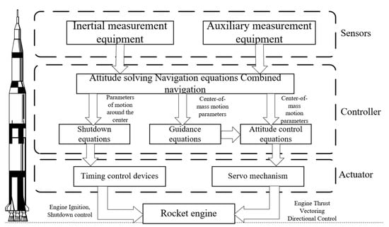
Figure 1.
Guidance and control diagram of the launch vehicle.
2.1. MBSE Modeling Process
MBSE refers to the establishment of a unified formal model, which involves the entire development process from the conceptual design stage to product realization and life cycle, to support system requirements, design, analysis, verification, and validation activities. The MBSE model shall acquire, manage, and provide access to all system and program data and their relationships. Its key characteristics are requirements and the internal and external interaction relationships of various data items.
As illustrated in Figure 2, the modeling method used in this paper is based on the MagicGrid method, which is specially used for systems engineering applications. During the MBSE modeling process, this paper initially uses user indices as the primary input to conduct a comprehensive requirement analysis tailored to stakeholders. Through iterative cycles, preliminary system requirements are shaped, and a preliminary system model is established to complete the schematic demonstration phase. Further analysis of the logical composition is then carried out, and the physical architecture is defined during the process of unpacking high-level requirements, which serves as input for subsequent engineering stages. Ultimately, the system is verified through simulation and testing against predefined test criteria and scenarios, and system requirements are traced back to close the loop. The whole process can be summarized in the following steps:
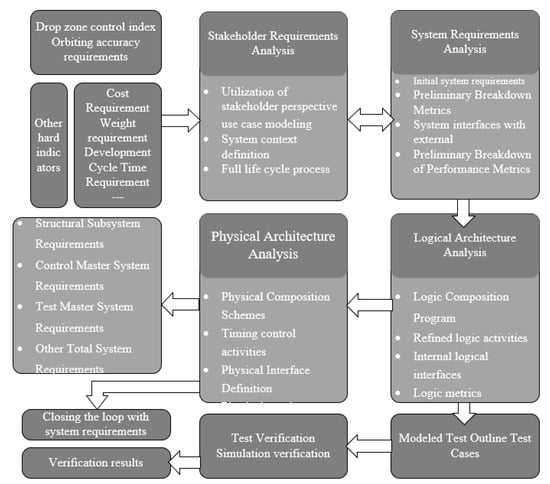
Figure 2.
MBSE modeling process diagram.
- (a)
- Requirement Elicitation and Analysis;
- (b)
- Logical Architecture Definition;
- (c)
- Physical Architecture Specification;
- (d)
- Simulation and Verification;
- (e)
- Iterative Refinement.
2.2. Navigation Guidance System Modeling
In this section, the MBSE method—implemented with MagicDraw 2021x using the MagicGrid methodology—is applied to analyze user requirements, define system functions, and perform design synthesis and system verification in the early development of the navigation and guidance system. First, the information of stakeholders related to the system construction scheme is obtained through the analysis of top requirements. This information includes the main user requirements, government regulations, industry standards, policies, and internal guidelines related to the system.
After analysis, the top-level requirement of the navigation guidance system is to design the guidance system of the launch vehicle, which is used to guide the vehicle to the target orbit. Combined with the characteristics of the mission and the decomposition of the top-level requirements, it is concluded that the requirements of the stakeholders can be divided into 12 aspects, including sensing the launch point parameters, initial alignment requirements, launch signal requirements, data transmission requirements, orbit entry accuracy requirements, six-degree dependability requirements (reliability, maintainability, safety, testability, supportability, and environmental adaptability), economic constraints, development cycle constraints, management requirements, self-inspection requirements, interface requirements, and flight information acquisition requirements.
In the model, each requirement has a unique identifier, name, and text specification. The entire list of stakeholder requirements can be displayed in a SysML requirement diagram, as shown in Figure 3.
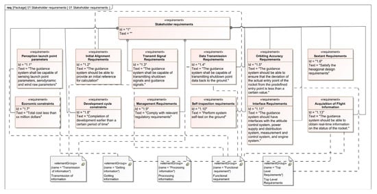
Figure 3.
Stakeholder requirement diagram.
During the process of requirement analysis, it is very crucial to describe the system requirements using use case diagrams. Use case diagrams can refine the stakeholder requirements into scenarios, telling people more precisely what they want to achieve from the system and what they want to achieve through the system. As shown in Figure 4, users in the use case diagram include the flight environment, power supply and distribution system, attitude control system, engine system, and test and launch control system, and the diagram can also be used to analyze each module in detail. In order to further describe the activity process of guiding the effective load to the orbit insertion point in use, the activity diagram of the guidance process is refined and designed as shown in Figure 5.
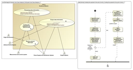
Figure 4.
Use case scenario diagram.
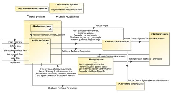
Figure 5.
System context analysis.
When constructing the requirement model, in order to complement the interactive elements in the use case model, including other external systems and users (human, organization, etc.), system context analysis will be further carried out. The system context determines the external view of the system, aiming at introducing elements that do not belong to the system but interact with it. As shown in Figure 5, the context of the guidance system includes an attitude control system, navigation system, and timing system.
The functional activities and non-functional activities based on the use case scenario provide support for in-depth analysis of system behavior, and the system context analysis lays foundation for the construction of the entire system’s requirement model. A complete requirement model not only needs to define what the system can do, that is, the functional requirements of the system, but also needs to analyze and define the non-functional requirements of the system, including performance requirements, six-character requirements, interface requirements, etc.
To ensure the integrity of the requirements model, it is necessary to trace the requirements and form a requirement traceability matrix. This can ensure that each requirement is fully analyzed and tracked throughout the development process. This paper traces the functional requirements using the system use case scenarios and links the preliminary requirements of the system with the system; the functional requirements of the system effectively implement good support for the scenarios constructed in the use case analysis, and the traceability of the system requirements assigned to the system context is realized, which ensures that the top-level requirement traceability runs through the entire project design process. The traceability matrix is shown in Figure 6 and Figure 7.
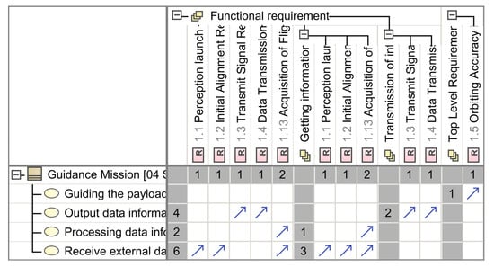
Figure 6.
Functional requirement traceability matrix diagram.
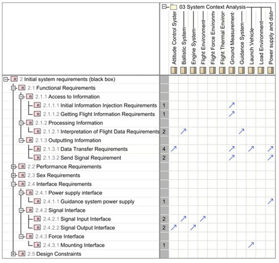
Figure 7.
System requirement traceability matrix diagram.
After the system requirements are initially determined, it is crucial to conduct a logical architecture analysis of the system in order to derive a specific solution. The purpose of the logical architecture is to capture the logical components within the system and to describe in detail the logical activities between the components and the internal logical interfaces. The logical architecture of the guidance system includes the measuring device, the communication device, the resolving device, and the data parameters contained therein.
Similarly to the goal of logical architecture analysis, the physical architecture is also a necessary part of the solution. The difference is that the technical choices involve specific physical components, added on the basis of the previous logical architecture analysis, and these physical components correspond to the logical architecture composition. The measuring device contains a GNSS and a gyroscope, while the communication device and the solving device contain the on-board computer. Each physical component will clarify the design parameters in the design process, such as the strapdown sampling cycle of the on-board computer and the inertial measurement unit (IMU) comprising accelerometers and gyroscopes. As shown in Figure 8, its output is the final architecture of the system.
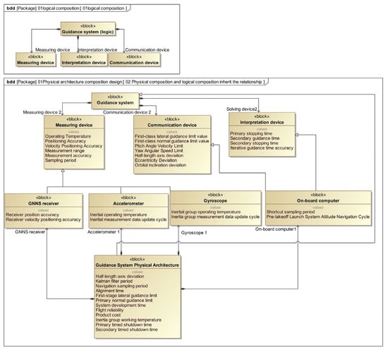
Figure 8.
Logical composition and physical architecture diagram.
3. Launch Vehicle Guidance Design
The task of the guidance system of the launch vehicle is to make the effective load of the launch vehicle enter the predetermined orbit and to ensure the accuracy of the orbit elements at the satellite orbit insertion point. In order to achieve this function, on the one hand, it is necessary to solve the real-time flight state of the rocket through the navigation system; on the other hand, it is necessary to give instructions to change its thrust vector and control the engine ignition and shutdown according to the requirements.
The guidance mode of the launch vehicle involved in this study is a composite guidance mode, which uses the perturbation guidance and iterative guidance methods to calculate guidance rate in segments. Perturbation guidance is used during the first-stage flight of the launch vehicle, and iterative guidance is used during the second-stage flight of the launch to improve the accuracy of orbit entry [3].
3.1. Perturbation Guidance Method
Under the action of perturbation, the rocket will deviate from its trajectory. For the analysis of perturbation, the perturbation method is used, the essence of which is to expand the actual trajectory near the standard trajectory and take the first-order term for study. When the interference is not too large, it can be regarded as a perturbation near the standard trajectory.
Taking the first-stage range as an example, the first-stage range is a function of the state parameters of the first-stage shutdown point (including seven state variables: velocities, positions, and time). That is,
According to perturbation theory, it is expanded in Taylor series near the standard trajectory. Let be the standard trajectory parameter and be the perturbation.
Since is much less than , the series converges. The higher order terms can usually be neglected, leaving only the first-order term.
Taking the pitch channel guidance as an example, its program pitch angle, actual pitch angle, and guidance quantity relationship formula is
where is the actual pitch angle, is the program pitch angle, and is the guidance quantity. The guidance quantity is calculated based on the velocity and position parameters of the rocket under the actual trajectory and the standard trajectory. It can be seen from the above formula that the sum of the program pitch angle and the guidance target quantity is the actual pitch angle. The main process is shown in Figure 9.
Figure 9.
Perturbation guidance process.
The upper half of Figure 9 depicts the five-step perturbation–guidance computation flow: the navigation guidance system feeds the current flight state into the perturbation guidance module, and the computed reference (program) angles are then forwarded to the attitude-control module, which in turn drives the six-degree-of-freedom rocket dynamics model [31], thereby closing the control loop. In the process of perturbation guidance calculation, the guidance quantity should include two parts, velocity guidance and position guidance. When there is only velocity, under the action of disturbance force and disturbance torque, the velocity error does not increase with time t, but there is a static error, and the position error increases time, which is the result of velocity guidance. When there is only position guidance, under the action of disturbance force and disturbance torque, the position error shows an oscillating trend, and the velocity error also oscillates accordingly, which shows that only position guidance is not sufficient. The disturbed motion oscillates back and forth on the standard trajectory, so it is necessary to form a mixed guidance command of velocity and position, and the command is as follows:
where is the static amplification coefficient, is the pitch guidance coefficient, and is the difference between the state variables of the rocket at the shutdown point and the standard trajectory after being disturbed. In engineering, in order to facilitate implementation, the guidance coefficients are generally calculated according to the values obtained near the point, and then a large number of trials are carried out to adjust them empirically, so as to finally achieve the highest guidance accuracy under the influence of disturbances.
3.2. Iterative Guidance Method
Perturbation guidance is to control the rocket to fly near the pre-designed standard trajectory, which has the advantages of a simple algorithm and small calculation amount for the guidance computer, but the disadvantages of a large amount of ground design and the need to adjust multiple guidance coefficients. Moreover, due to the use of small perturbation assumption, the guidance accuracy is poor in the case of large perturbations.
Iterative guidance is an explicit guidance method that defines a set of shutdown conditions according to the mission requirements and issues a shutdown command when the conditions are met. This guidance problem belongs to a high-dimensional two-point boundary value problem. In order to fully improve the utilization of rocket fuel, the shortest flight is generally taken as the performance index, and the optimal control theory is used for guidance to find its optimal flight trajectory. Iterative guidance does not rely on a predetermined program. Whether the predetermined range or the required speed, orbit period, and other parameters are used as the shutdown control function, iterative guidance requires real-time calculation according to the function and the current motion parameters of the rocket and real-time calculation of the optimal flight trajectory, so it has strong flexibility and adaptability, allowing the actual flight to deviate greatly from the predetermined standard trajectory, and still has high guidance accuracy under large disturbances.
Taking the pitch channel as an example, the expression of the optimal control angle can be obtained by using the analytical solution method of the optimal control problem:
where is the control angle that satisfies the velocity vector of the target point, and and are the additional control angle quantities generated by the position of the target point.
The iterative guidance calculation process is shown in Figure 10.
Figure 10.
Iterative guidance process.
The remaining flight time needs to be solved by iteration. First, set the convergence accuracy . Choose an initial value (usually the convergence of the previous guidance cycle) and substitute it into the above formula to obtain a new . When the convergence condition is satisfied, stop the iteration and record convergence value as for subsequent calculations.
The final optimal pitch angle can be obtained:
where is the sampling frequency.
During the flight of the launch vehicle, the above process needs to be repeated continuously until the launch vehicle meets the shutdown characteristic quantity.
3.3. Launch Vehicle Guidance Model
Section 3.1 and Section 3.2 presented the perturbation guidance and iterative guidance components of the combined guidance scheme; this section describes the end-to-end simulation model used for guidance design. Because the study is intended for the conceptual phase of launch vehicle guidance development, the following simplifying assumptions are adopted in the dynamic simulation:
- (1)
- The Earth is treated as a spherical, non-rotating mass point; hence, the gravity model contains no perturbative terms.
- (2)
- Engine start-up transients, tail-off thrust, and time-varying mass-flow rates are neglected.
- (3)
- Small-offset thrust equations are omitted. Within the atmosphere, thrust is modeled as the nominal vacuum thrust reduced by nozzle exit pressure effects; outside the atmosphere, only nominal vacuum thrust is applied.
- (4)
- The instantaneous equilibrium assumption is employed: aerodynamic and control torques are ignored, and attitude changes are assumed to occur instantaneously.
Based on these assumptions, the complete simulation workflow is established as follows.
The simulation object is the navigation-and-guidance model. Its role in the closed loop is to acquire the instantaneous flight state (position, velocity, and mass), compute the control command or optimal attitude required to reach the target orbit, and pass this information downstream to the attitude control model.
A MATLAB 2019 ode 45 integrator is used for the launch vehicle dynamics. The integrator replaces the navigation module; its outputs—position, velocity, and mass—are used directly as the flight-state variables for the guidance algorithm, as shown in Equation (6):
where is the state equation of the flight-state variables , its time derivative , and the parameters .
Our focus is on guidance algorithms; the simulation employs the same algorithms used in engineering practice.
Atmospheric phase: Perturbation guidance supplies the control command. The governing equation is given in Equation (7).
The resulting command is forwarded to the attitude control model.
Exo-atmospheric phase: Iterative guidance yields the optimal attitude angles. The governing equation is given in Equation (5). These angles are likewise transmitted to the attitude control model.
Using the current attitude and the guidance-derived reference, the attitude control model performs control allocation and issues commands to the engines. Because the navigation-and-guidance model does not include actuators, the simulation adopts the instantaneous equilibrium assumption: attitude changes are considered to occur in zero time, thereby simplifying the attitude control portion of the algorithm.
4. System Simulation Verification
In the design process of the launch vehicle guidance system, the landing point of its sub-stage and the final orbit entry accuracy are important indicators to whether the design of the navigation guidance system meets the requirements. It takes a long time and high cost to manufacture a real launch vehicle to verify the navigation guidance system, it is also inconsistent with the actual engineering situation. Therefore, it is necessary to use computers to simulate and analyze the virtual prototype. On the basis of the architecture model of the navigation guidance system, this paper carries out joint simulation and closed-loop verification of the system index in combination with the domain model. At the same time, the advantages of the rapid iterative design of the SysML model are combined with the precise model of navigation guidance to carry out trade-off analysis and the optimal guidance scheme under different parameter combinations.
In order to verify the design index of the navigation guidance system, it is necessary to carry out the dynamic modeling of the carrier rocket. In this, the guidance system is designed by using the combined guidance method. The perturbation guidance method is used in the flight stage of the carrier rocket in the atmosphere, and the iterative guidance method is used in the flight stage outside the atmosphere. In the simulation model, the control effect is changed by adjusting the design parameters of the guidance system, as to achieve the design index of the system. The design parameters of the guidance system are shown in Figure 11.
Figure 11.
Guidance design parameter diagram.
However, when performing multi-condition simulation tasks in MATLAB, only one condition’s simulation results can be obtained at a time, which means a lot of is needed to adjust the program. This process leads to high labor costs, and the results obtained are not intuitive enough for comparison. The advantage of SysML models is they can quickly adjust simulation conditions and integrate multiple subsystems for simulation, compensating for the difficulty of performing multi-condition simulations when using simulation software alone. This paper integrates SysML system architecture models with domain models for simulation, as shown in Figure 12.
Figure 12.
SysML simulation process diagram.
In the MBSE model, the input of the simulation guidance model based on MATLAB is parameterized, and the overall parameters of the launch vehicle, the launch site, the target orbit, and other information are used as the input for the simulation model. The simulation results are obtained by calling the functions in MATLAB. In Figure 12, modules labeled “Standard Ballistic Information”, “Guidance Program”, and “Drop Zero Solver” are capable of performing trajectory, guidance, and landing point calculation functions for the launch vehicle. These calculation modules obtain parameters from upstream reading modules via MagicDraw models. Within the calculation modules, the MATLAB language is selected, and interactions between MagicDraw and MATLAB are achieved through MATLAB’s function calls, thereby determining compliance with mission requirements.
Figure 13 shows the detailed activity diagram of the GNC system. This includes an innovative method for data exchange between Magic Draw software and MATLAB software. In order to achieve closed-loop feedback control of the rocket, the single-step data exchange technique is shown in Figure 14a–d. The Magic Draw software calls the MATLAB programs of the rocket dynamics model, navigation model, guidance model, and attitude control model through behavior attribute programming in the Call Behavior Action module and returns the MATLAB calculation results to the Magic Draw software for the next flight program calculation.
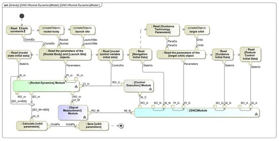
Figure 13.
Detailed activity diagram of the GNC system.
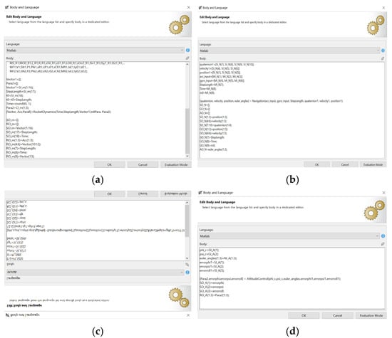
Figure 14.
Diagrams of data exchange (a) to rocket dynamics model; (b) to navigation model; (c) to guidance model; and (d) to attitude control model.
This paper establishes a mission scenario for a launch vehicle, with the accuracy of the sub-stage landing point and the accuracy of orbit insertion as the basis judging whether the navigation and guidance system design meets the requirements. The mission scenario is as follows: a three-stage launch vehicle with boosters is taken as the research object, and the rocket is guided by the navigation and guidance system to bring the effective load into the sun-synchronous orbit (SSO), and the orbit elements are shown in Table 1. All vehicle mass properties, thrust profiles, and stage-sequence parameters are taken directly from ref. [31].

Table 1.
Orbital elements of the target orbit.
The launch took place at the Taiyuan Satellite Launch Center, with the launch point parameters shown in Table 2.
Table 2.
Launch point parameters.
In the process of guidance simulation, it is generally assumed that the carrier rocket is not affected by any disturbances, and a standard trajectory is designed with sub-stage impact points and extremely high orbit insertion accuracy. Subsequently, disturbances are added, and the results without control and with control are compared to verify the guidance of the navigation guidance system. The disturbances in the guidance simulation process mostly take the influence of flight environmental factors and the deviation of the overall parameters of the rocket itself. This paper focuses on guidance performance under crosswind conditions. The wind field model is a stochastic, three-component field defined in the ground coordinate system [32]:
where is the altitude in meters, wind speed is the relative speed of the atmosphere to the ground, is the wind azimuth angle relative to the ground x-axis, and is the angle between the direction of wind speed and the y-axis in the plane of y–z. To ensure robustness, the design phase assumes an extreme wind speed of 40 m/s.
As shown in Table 3, it can be observed that under interference conditions, the semi-major axis deviation without guidance reaches 0.4372%, the eccentricity deviation is 0.012724, and the orbital inclination deviation is 0.2202%. The landing lateral deviation is approximately 1000 m, and the longitudinal deviation is about 700 m. After the guidance system is applied, the flight accuracy is improved, especially with the semi-major axis deviation reduced to 0.0116%, the eccentricity deviation minimized to 0.004657, and the landing lateral deviation reduced to 27 m. Compared to the unguided interference trajectory, this demonstrates that the guidance method presented in this paper has excellent adaptability and reliability in the control of launch vehicles.
Table 3.
Verification of guidance effects.
5. Parameter Trade-Off Analysis
In the process of guidance system design, the selection of design parameters in the guidance algorithm is key to determining whether the system meets the requirements. For perturbation guidance algorithms, the design parameters include the guidance coefficient, the start guidance time, and the guidance time. For iterative guidance algorithms, the parameters include the initial value of the remaining shutdown time, the accuracy of the remaining shutdown time, etc. These parameters are confirmed by the developers of the guidance system. In the traditional engineering design process, developers adjust the parameters empirically through a large number of trials in simulation software and finally achieve the highest guidance accuracy. However, during the trial process, developers need to manually adjust the parameters and often can only adjust one parameter at a time, making it difficult to consider the and combination of different parameter adjustment processes. This paper simulates the SysML system architecture model and domain model together, extracts the design parameters as the input of the simulation, uses the advantage that the SysML model can perform multi-input trade-off research to input multiple sets of data into the simulation model, and then selects the best set of design parameters according to specific indicators, as shown in Table 4.
Table 4.
List of indicators.
5.1. Determine the Design Parameters and Indicators
The guidance method used in this paper is a combined guidance method, which includes perturbation guidance and iterative guidance. The writing process of the two guidance types contains many parameters, but not all parameters can be adjusted to change the guidance effect. Therefore, before the trade-off study, it is necessary to determine the design parameter evaluation indicators. The design parameters initially confirmed by the trade-off study are shown in Table 5.
Table 5.
Parameter list.
5.2. Contribution Analysis
In the process of confirming the design parameters of perturbation guidance, the evaluation index is mainly the lateral and longitudinal deviation of the sub-stage landing point. In this paper, combined with the experience of the previous trial calculation, it is found that the adjustment of some design parameters of perturbation guidance has no obvious effect on the landing point deviation. Therefore, in order to reduce the unnecessary calculation amount, improve the efficiency of optimization design, and carry out the trade-off study pertinently, this paper uses the contribution analysis method to screen the preliminarily confirmed perturbation guidance design parameters and six guidance coefficients and selects the key coefficients for study.
Contribution analysis requires accurate and rich samples. This paper gives a set of coefficient combinations obtained from preliminary trials as initial values. Each coefficient takes 0.3 times and 0.7 times the initial value as the maximum and minimum value, respectively. The three types of values obtained are orthogonally designed to obtain 8 groups of samples. Firstly, the samples need to be normalized, as shown in Equation (6):
is the i-th sample, is the mean of the samples, is the standard deviation of the samples, and is the total number of the samples. Then, based on the normalized samples, the mathematical relationship between the input and the output is fitted by a polynomial approximation expression, and its formula is as follows:
is the value of the objective function, is the number of variables, is the constant term, is the coefficient of the linear main effect, is the coefficient of the interaction effect, and is the interaction effect and error between the multivariate. can represent the contribution degree of each design to the response.
To better show the contribution of each design variable to the response, the contribution of each variable is quantified by using a percentage, as shown in the following formula:
The initial values of the coefficients are shown in Table 6.
Table 6.
Coefficient initial value.
The guidance algorithm was simulated with the perturbation guidance coefficients in the guidance law according to the 27 sets of samples determined, and the simulation was recorded.
Subsequently, the samples were normalized, and the contribution of each coefficient to the lateral and longitudinal deviation of the sub-stage impact point was calculated with the data, with the results shown in blue column in Figure 15 and Figure 16.
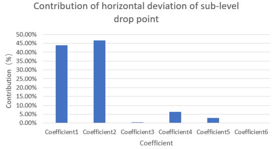
Figure 15.
Contribution of lateral deviation of sub-level landing point.
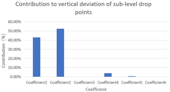
Figure 16.
Contribution of longitudinal deviation of sub-level landing point.
The contribution of coefficient 3 and coefficient 6 to the lateral deviation of the sub-level landing point is less than 1% in Figure 15, and the contribution to the longitudinal deviation is less than 0.5% in Figure 16. Coefficient 1 , coefficient 2 , coefficient 4 , and coefficient 5 have a higher contribution to the landing point deviation compared to the other two coefficients and have a greater impact on the landing point accuracy, so they are focused for improvement and optimization in the subsequent trade-off analysis. Coefficient 3 and coefficient 6 , which have less impact on the landing point accuracy, are no longer included in the subsequent trade-off analysis.
5.3. Weighted Analysis
The advantage of the SysML model is that it can input multiple sets of data for the joint simulation model. After the contribution analysis of the input parameters, the finally confirmed input parameters for perturbation guidance are the X-direction velocity guidance coefficient, Y-direction velocity guidance coefficient, X-direction position guidance coefficient, and Y-direction position guidance coefficient, while for iterative guidance, they are the remaining shutdown time initial value and remaining shutdown time accuracy. The evaluation indicators for perturbation guidance are sub-level landing point lateral deviation and longitudinal deviation, while for iterative guidance, they are orbit semi-major axis deviation, eccentricity deviation, and orbit inclination deviation.
This paper makes a trade-off analysis of perturbation guidance and iterative guidance, respectively, and the input parameters involved in perturbation guidance are 4, with the corresponding parameter values given in the previous section taken as the initial values of the 4 input parameters, as shown in Table 7.
Table 7.
Initial values of the final coefficients.
These initial values are obtained by preliminary trial calculation and engineering experience, which can achieve better guidance effects. In this paper, for perturbation guidance, the weight analysis of each type of coefficient takes 5 sample values, which are 95%, 97.5%, 100%, 102.5%, and 105% of the initial value. The permutation and combination of these 4 types of coefficients are carried out to obtain 65 groups of samples as the input data of the joint simulation model, as shown in Figure 17.
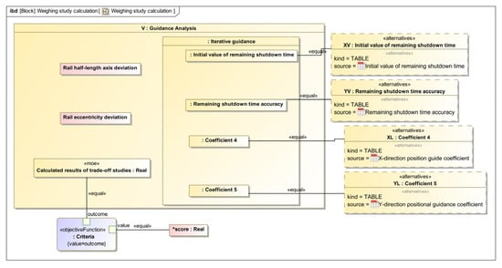
Figure 17.
Perturbation guidance weight analysis model diagram.
The SysML model will automatically carry out joint simulation for each group of data samples and output the evaluation index. The results of the perturbation guidance weight analysis are shown in Figure 18.
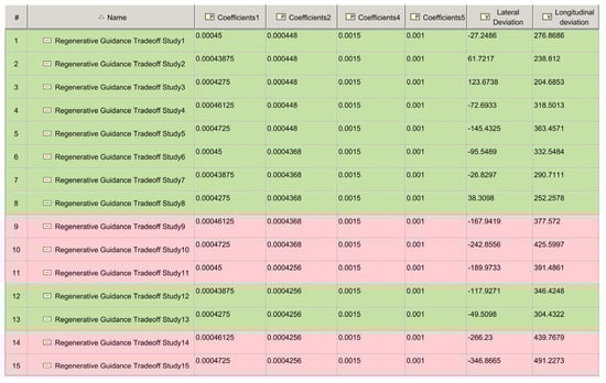
Figure 18.
Perturbation guidance weight analysis result chart.
This paper uses an absolute lateral deviation of less than 150 m and an absolute longitudinal deviation of less than 35 m as the index conditions for screening, and the parameter combination that meets the index in the figure will be marked as green, while the parameter combination that does not meet the index marked as red.
There are two input parameters involved in iterative guidance, which are the initial value of the remaining shutdown time and the accuracy of the remaining shutdown time. The initial value of the input parameters is given by the previous trial calculation and engineering experience, as shown in Table 8.
Table 8.
Initial values of the iterative guidance parameters.
This paper selects 11 sample values for each type of parameter in the trade-off analysis of iterative guidance, which are 95%, 96%, 97%, 98%, 99%, 100%, 101%, 102%, 103%, 104%, and 105% of the initial value. The permutation and combination of these two types of data are used to obtain 121 groups of samples as input data, and the orbit injection accuracy is used as the evaluation index. The analysis model diagram is shown in Figure 19, and some of the results after the trade-off analysis are shown in Figure 20.
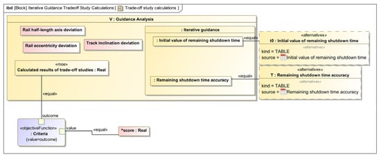
Figure 19.
Iterative guidance weight analysis model diagram.
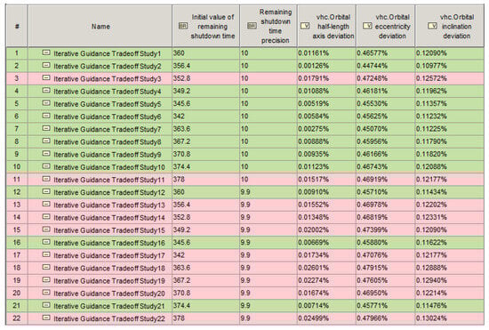
Figure 20.
Iterative guidance weight analysis result chart.
The results of the iterative guidance weight analysis are filtered with the conditions of orbit accuracy deviation less than 0.01%, eccentricity deviation less than 0.047%, and orbit inclination deviation less than 0.121%. The parameter combinations that meet the indicators are displayed in green, and the combinations that partially meet or do not meet are displayed in red.
From the results of the observation weight analysis, it can be seen that the parameter combination obtained by the previous trial calculation and engineering experience is not the combination for the guidance effect. For perturbation guidance, the best combination can be obtained by selecting the initial value of the coefficient 1 as 95%, coefficient 2 as 100%, coefficient 4 as 102.5% and coefficient 5 as 100%, which results in the smallest sub-level landing point deviation. For iterative guidance, the best combination can be obtained by selecting the initial value of the remaining shutdown time as 9% and the initial value of the remaining shutdown time accuracy as 101%, which results in the smallest orbit entry deviation.
6. Conclusions
This study concentrates on the guidance system design for launch vehicles, employing MBSE methodology to conduct comprehensive system modeling, integrated simulations, and trade-off analyses.
Following the completion of a four-dimensional framework model encompassing requirements, functions, logic, and physical architecture for the navigation system, we established a specialized simulation model for the guidance system. This enabled the implementation of MBSE-integrated simulations that effectively combine domain-specific professional models, thereby achieving closed-loop verification of system requirements.
Building upon the integrated simulation platform, we conducted parametric sensitivity analyses to identify critical factors influencing launch vehicle performance. By leveraging the dual advantages of rapid iteration capability and high precision inherent in professional domain models, this research systematically compares parameter configurations under various mission scenarios. Through this approach, optimal parameter selections were determined, resulting in minimized orbital insertion errors.
The study ultimately completes the trade-off analysis for guidance system design, demonstrating a methodology that effectively bridges theoretical modeling with practical engineering implementation.
Author Contributions
Conceptualization, Z.J. and W.Z.; methodology, K.Y.; software, Y.J.; validation, Z.J., W.Z., and S.L.; formal analysis, H.L.; investigation, K.Y.; resources, S.L.; data curation, H.L. and Y.J.; writing—original draft preparation, K.Y.; writing—review and editing, Z.J.; supervision, Z.J.; project administration, W.Z.; funding acquisition, W.Z. All authors have read and agreed to the published version of the manuscript.
Funding
This research was funded by the Defense Industrial Technology Development Program (Grant No. JCKY2023203A002).
Data Availability Statement
No new data were created or analyzed in this study. Data sharing is not applicable to this article.
Conflicts of Interest
No potential conflict of interest was reported by the authors.
References
- Lu, P. What is guidance? J. Guid. Control Dyn. 2021, 44, 1237–1238. [Google Scholar] [CrossRef]
- Farrior, J.; Roberson, R. Guidance and Control; American Institute of Aeronautics and Astronautics: New York, NY, USA, 1962. [Google Scholar]
- Ma, W. Review and prospect of missile/launch vehicle guidance, navigation and control technologies. J. Astronaut. 2020, 412, 860–867. [Google Scholar]
- Wang, D.; Liang, H.; Cui, J. Modeling and simulation of top-level design based on MBSE. J. Phys. Conf. Ser. 2020, 1486, 72061. [Google Scholar]
- Xiao, J.; Zhou, X.; Li, J.; Zhang, Q.; Sun, S. Propulsion critical system design for launch vehicle by model-based systems engineering. Missiles Space Veh. 2023, 2023, 37–42. [Google Scholar]
- Oroz, J.; Roohi, Z.; Abelezele, S. Implementing the digital thread—A proof-of-concept. In Proceedings of the AIAA SCITECH 2023 Forum, National Harbor, MD, USA, 23–27 January 2023; American Institute of Aeronautics and Astronautics: Reston, VA, USA, 2023. [Google Scholar]
- Wang, W.; BI, W.; Zhang, A.; Fan, Q. Functional modeling method of civil aircraft system based on MBSE. Syst. Eng. Electron. 2021, 43, 2884–2892. [Google Scholar] [CrossRef]
- Nichols, D.; Lin, C. Integrated Model-Centric Engineering: The Application of Mbse at Jpl Through the Life Cycle; INCOSE International Workshop MBSE Workshop: Los Angeles, CA, USA, 2014. [Google Scholar]
- Delligatti, L. Sysml Distilled: A Brief Guide to the Systems Modeling Language, 1st ed.; Addison-Wesley Professional: Boston, MA, USA, 2013. [Google Scholar]
- Taraila, W.; Asundi, S. Model-based systems engineering for a small-lift launch facility. Syst. Eng. 2022, 25, 537–550. [Google Scholar] [CrossRef]
- Weiland, K.; Holladay, J. Model-Based Systems Engineering Pathfinder: Informing the Next Steps; INCOSE International Symposium: Adelaide, Australia, 2017; pp. 1594–1608. [Google Scholar]
- He, W.; Hu, J.; Zhao, T.; Peng, Y.; Tang, J. Research on model based launch vehicle overall design. Missiles Space Veh. 2021, 378, 12–17. [Google Scholar]
- Wang, T.; Tan, C.; Huang, L. Simplexity testbed: A model-based digital twin testbed. Comput. Ind. 2023, 145, 103804–103821. [Google Scholar] [CrossRef]
- Liu, S.; Li, W.; Zhang, W. Iterative feedback design of de laval nozzle. In Proceedings of the 1st International Conference on Mechanical System Dynamics (ICMSD), Nanjing, China, 24–27 August 2022; pp. 1429–1434. [Google Scholar]
- Madni, A.; Purohit, S. Augmenting MBSE with digital twin technology: Implementation, analysis, Preliminary Results, and Findings. In Proceedings of the 2021 IEEE International Conference on Systems, Man, and Cybernetics (SMC), Melbourne, Australia, 17–20 October 2021; IEEE: Piscataway, NJ, USA, 2021; pp. 2340–2346. [Google Scholar]
- Madni, A.; Purohit, S. Economic analysis of model-based systems engineering. Systems 2019, 7, 12. [Google Scholar] [CrossRef]
- Bajaj, M.; Cole, B.; Zwemer, D. Architecture to geometry—Integrating system models with mechanical design. In Proceedings of the AIAA SPACE, Long Beach, CA, USA, 13–16 September 2016; American Institute of Aeronautics and Astronautics: Reston, VA, USA, 2016; pp. 1453–1471. [Google Scholar]
- Ko, A.; Keel, W.; Beale, J. ModelCenter MBSE for OpenMBEE: MBSE analysis integration for distributed development. In Proceedings of the AIAA AVIATION 2022 Forum, Chicago, IL, USA, 27 June–1 July 2022; American Institute of Aeronautics and Astronautics: Reston, VA, USA, 2022; pp. 1–20. [Google Scholar]
- Huang, P.; Peng, Q.; Wu, X.; Ni, Q. Architecture modeling for manned lunar landing mission based on DoDAF. Syst. Eng. Electron. 2023, 45, 2131–2137. [Google Scholar] [CrossRef]
- Miao, X.; Dong, X.; Qian, Z.; Hu, Y.; Li, M. Architecture modeling of aviation equipment intelligent support system based on DoDAF. Syst. Eng. Electron. 2024, 46, 640–648. [Google Scholar] [CrossRef]
- Wang, Y.; Bi, W.; Zhang, A. DoDAF-based civil aircraft MBSE development method. Syst. Eng. Electron. 2021, 43, 3579–3585. [Google Scholar] [CrossRef]
- Mao, Z.; Qu, Z.W.; Zhang, T.; Lu, Y.; Fu, S.; Huang, D. Design of civil aircraft certification test flight scenario based on MBSE. Syst. Eng. Electron. 2020, 42, 1768–1775. [Google Scholar] [CrossRef]
- Li, D.; Bi, W.; Zhang, A.; Fan, Q. MBSE-based process management in the development of civil aircraft. Syst. Eng. Electron. 2021, 43, 2209–2220. [Google Scholar] [CrossRef]
- Zhang, X.; Wu, B.; Zhang, X.; Duan, J.; Wan, C.; Hu, Y. An effective MBSE approach for constructing industrial robot digital twin system. Robot. Comput.-Integr. Manuf. 2023, 80, 102455–102474. [Google Scholar] [CrossRef]
- Jia, Z.; Lu, F.; Wang, H. Multi-stage attack weapon target allocation method based on defense area analysis. J. Syst. Eng. Electron. 2020, 31, 539–550. [Google Scholar] [CrossRef]
- Zhang, W.; Liu, Z.; Liu, X.; Jin, Y.; Wang, Q.; Hong, R. Model-based systems engineering approach for the first-stage separation system of launch vehicle. Actuators 2022, 11, 366. [Google Scholar] [CrossRef]
- Liu, Z.; Chen, Q.; Xia, N.; Yang, M.; Du, Q.; Lu, J. An MBSE tool to support architecture design for spacecraft electrical power system. INCOSE Int. Symp. 2018, 28, 64–78. [Google Scholar] [CrossRef]
- Caballes, M.; Odita, T.; Chen, G. Implementation of MBSE approach for developing reliability model to ensure robustness of sounding rocket program using made modeling tool. In Proceedings of the 9th Annual World Conference of the Society for Industrial and Systems Engineering, Johor Bahru, Malaysia, 17–18 September 2020; pp. 140–147. [Google Scholar]
- Ma, J.; Wang, G.; Lu, J.; Vangheluwe, H.; Kiritsis, D.; Yan, Y. Systematic literature review of MBSE tool-chains. Appl. Sci. 2022, 12, 3431. [Google Scholar] [CrossRef]
- Xu, Z. Construction of tool chains for civil aircraft design based on MBSE method. Aeronaut. Manuf. Technol. 2017, 5, 100–104. [Google Scholar]
- Zhang, W. Dynamics and Control of Launch Vehicles; Astronautics Publishing House: Beijing, China, 2015. [Google Scholar]
- Li, W.; Yan, H.; Zhang, W. Trajectory simulation of a certain type of missile under wind disturbance. Comput. Technol. Dev. 2011, 21, 246–249. [Google Scholar]


Disclaimer/Publisher’s Note: The statements, opinions and data contained in all publications are solely those of the individual author(s) and contributor(s) and not of MDPI and/or the editor(s). MDPI and/or the editor(s) disclaim responsibility for any injury to people or property resulting from any ideas, methods, instructions or products referred to in the content. |
© 2025 by the authors. Licensee MDPI, Basel, Switzerland. This article is an open access article distributed under the terms and conditions of the Creative Commons Attribution (CC BY) license (https://creativecommons.org/licenses/by/4.0/).