Research on Path Tracking Technology for Tracked Unmanned Vehicles Based on DDPG-PP

Abstract

Realizing path tracking is crucial for improving the accuracy and efficiency of unmanned vehicle operations. In this paper, a path tracking hierarchical control method based on DDPG-PP is proposed to improve the path tracking accuracy of tracked unmanned vehicles. Constrained by the objective of minimizing path tracking error, with the upper controller, we adopted the DDPG method to construct an adaptive look-ahead distance optimizer in which the look-ahead distance was dynamically adjusted in real-time using a reinforcement learning strategy. Meanwhile, reinforcement learning training was carried out with randomly generated paths to improve the model’s generalization ability. Based on the optimal look-ahead distance output from the upper layer, the lower layer realizes precise closed-loop control of torque, required for steering, based on the PP method. Simulation results show that the path tracking accuracy of the proposed method is better than that of the LQR and PP methods. The proposed method reduces the average tracking error by 94.0% and 79.2% and the average heading error by 80.4% and 65.0% under complex paths compared to the LQR and PP methods, respectively.

1. Introduction

As a core component of automated operation systems, unmanned vehicle technology is currently in a critical period of rapid development. In particular, tracked unmanned vehicles, with excellent terrain adaptability, are playing an increasingly important role in both military reconnaissance in complex terrain and disaster relief in difficult road conditions [1,2,3]. For tracked unmanned vehicles, the path tracking function aims to ensure that the vehicle can arrive accurately and follow the established path stably, and its tracking accuracy is directly related to the accuracy and efficiency of the operation, which is one of the most critical issues in this field. Therefore, in-depth investigation of tracking control algorithms for tracked unmanned vehicles is of great practical significance for improving the quality of operation and for promoting the realization of fully autonomous operation [4,5].

In general, a lot of practices and studies have been conducted previously. The path-tracking control methods proposed in related studies can be mainly categorized into three types: model-free methods, model-based methods, and geometry-based methods. Model-free control methods realize path tracking by simplifying the dynamic characteristics of the system and by relying on empirical regulation of the feedback signal. Wael proposed a Proportional Integral Differential (PID) controller for facilitating the longitudinal aspect of self-driving car tracks. Three different design approaches were used to find and tune the controller hyperparameters [6]. Anh et al. proposed an adaptive fuzzy PID method for non-complete autonomous mobile robots to follow a desired path, where the adaptive tuning of the PID controller is realized through a fuzzy controller [7]. Although these methods have advantages of a simple structure and intuitive parameter adjustment, their parameter tuning methods are largely dependent on experience, and, in trajectory tracking control, unsuitable parameters can lead to vehicle destabilization, which brings high testing costs and time consumption [8]. In addition, when the nonlinearity and uncertainty of the system are high, model-free control becomes unreliable due to its inability to accurately represent the motion state of the system [9]. To account for this limitation, model-based control methods construct a feedforward–feedback composite control architecture by introducing a vehicle/robot dynamics model to achieve improved dynamic response accuracy and disturbance resistance. Tao et al. proposed a feedforward + predictive LQR lateral control method that can improve the accuracy of distance error control and heading error control [10]. Wang et al. proposed an adaptive fuzzy LQR-based control strategy for optimizing the direct lateral deflection torque control of a distributed-drive electric vehicle [11]. Park et al. used the LQR method, combined with an adaptive preview distance scheme, to derive a dynamics model of the vehicle, and implemented path tracking control through an optimized design [12]. However, such methods are highly sensitive to the accuracy of the model parameters and the observability of external disturbances [13], and are prone to triggering control volume jitter under model mismatch or complex perturbation conditions [14], which constrains their robustness in unstructured environments. In this context, geometry-based path tracking methods transform path tracking into a geometric tracking problem by reconfiguring the problem perspective, which circumvents the bottleneck caused by model dependency from the bottom. The geometry-based approach of Pure Pursuit (PP) methods have unique physical intuition and engineering ease of use by controlling the heading angle of the vehicle to eliminate the lateral and heading errors between the current position and the desired position.

PP is a geometry-based control algorithm that has been studied by many scholars due to its simplicity and efficiency. Elbanhawi et al. proposed a model-predictive active yaw control implementation for PP path tracking that adapts to the steady-state lateral dynamic characteristics of a vehicle in order to improve its tracking performance at high speeds [15]. Jiang et al. proposed an enhanced PP path tracking algorithm for mobile robots that is optimized using NSGA-II with high-accuracy GNSS navigation for precise positioning [16]. However, the path tracking effect of the PP method is closely related to the selection of the look-ahead distance, and different values will directly lead to significant differences in the tracking effect. To address this problem, Sun et al. adaptively adjust the look-ahead distance based on the steering angle and deflection angle to improve the performance of the traditional PP algorithm [17]. Huang et al. establish a dynamic pre-scanning mechanism that integrates the vehicle speed and path geometry into the look-ahead distance calculation, which improves the adaptability of the algorithm to complex paths [18]. Ahn et al. place the forward target point out of the path based on the vehicle’s position, direction, and the curvature of the path, thus solving the problem of tracking the target point in the front of a vehicle placed outside the path, thus solving the tangency problem in path tracking; however, the generalization is limited, as the relevant parameters need to be adjusted when the curvature and speed change [19]. According to previous studies, look-ahead distance is affected by vehicle speed, path curvature, and other factors. Although these studies have made some progress in calculating look-ahead distance, there are still some problems to be solved. First, it is difficult to accurately describe the relationship between the influencing factors and the look-ahead distance through mathematical expressions, which leads to the selection of the look-ahead distance not being reasonable enough. Secondly, selection of the look-ahead distance does not fully consider the vehicle path connection, resulting in poor model adaptability.

Deep Reinforcement Learning (DRL), as an important branch of machine learning, has become an effective tool for solving complex continuous control problems by virtue of its advantage of combining deep neural networks to perceive the environment and reinforcement learning to make dynamic decisions [20,21]. Currently, DRL has achieved considerable results in the field of gaming [22], and has also been widely studied in some fields that require complex control, such as intelligent ships [23], unmanned surface vehicles [24], and driverless vehicles [25]. In the field of path tracking, researchers have tried to improve the control performance by using various DRL methods: Niu et al. proposed and implemented a preference-based reinforcement learning method for ROV path tracking [26]. Zhang et al. constructed a Deep Q-Network based on a 5-layer Back Propagation neural network to improve the path tracking accuracy of vehicles [27]. Chen et al. designed a non-complete wheeled robot path tracking controller based on DRL, and established the control strategy of the wheel line speed and steering speed using the Deep Deterministic Policy Gradient (DDPG) algorithm, and the experimental results show that the reinforcement learning method had higher computational efficiency and robustness compared to the MPC method [28]. The network architecture of DRL can learn from a large amount of data containing different driving conditions [29,30] and automatically excavate the complex and precise intrinsic connection between the influencing factors and the look-ahead distance. However, existing DRL-based path tracking methods still have the some problems, for example, the ‘black box’ nature of deep neural networks, which leads to the insufficient interpretability of strategies [31] and poor convergence stability after training [32]. Aiming at the above problems, a series of exploratory studies have been carried out in academia. Reference [33] proposed an adaptive robust framework based on Control Barrier Function (CBF), which embeds physical constraints into optimization objectives and improves the interpretability of the model. Reference [34] designed an event-triggered mechanism that updates the control variable only when the tracking error exceeds a threshold. Compared with traditional DRL, it reduces 40% of invalid calculations and improves the convergence speed of the algorithm. The above research provides a new idea for a solution to the path tracking problem. For this reason, this study proposes an architecture that combines DDPG with classical PP algorithms. The PP model is embedded into the framework as the basic control layer, and its explicit expression based on geometric kinematics can enhance the strategy interpretability; a priori knowledge of the kinematics of the PP model reduces the difficulty of the strategy search and effectively mitigates the problem of the stability of the traditional DRL training.

In summary, in this paper, with the goal of improving the path tracking accuracy of tracked vehicles, a path tracking scheme with hierarchical control is proposed by fusing the DDPG and PP methods. The proposed scheme is divided into two parts: the upper controller adaptively adjusts the look-ahead distance based on reinforcement learning according to the tracking error, heading error, and the velocity ratio between the left and right tracks; the lower controller calculates the required torque of the tracked vehicle based on the PP algorithm according to the look-ahead distance obtained from the upper layer to achieve stable tracking of a given path.

The main contributions of this paper can be summarized as follows.

• A DDPG-based upper controller is proposed to dynamically adjust and optimize the look-ahead distance, with the optimization objective of minimizing the path tracking error, which deals with the path tracking problem caused by unreasonable look-ahead distance in the PP algorithm of tracked vehicles.
• A random path generation mechanism is adopted, and the model is trained in a path environment containing various types of random curvature features, which prompts the model to deeply learn the look-ahead distance-adjustment strategies under different complex paths and improves the controller’s generalization ability and adaptability.
• A PP-based lower controller is proposed to accurately calculate the driving moments of the left and right tracks of a tracked vehicle to achieve the stable tracking of a tracked unmanned vehicle against a planned path.

The rest of the paper is organized as follows: Section 2 describes the tracked vehicle dynamics model used in this paper. Section 3 gives the theoretical background and the path tracking control system based on the DDPG-PP controller. Section 4 carries out path tracking tests to validate the proposed method and gives the test results and analysis. Finally, in Section 5, the main conclusions are given.

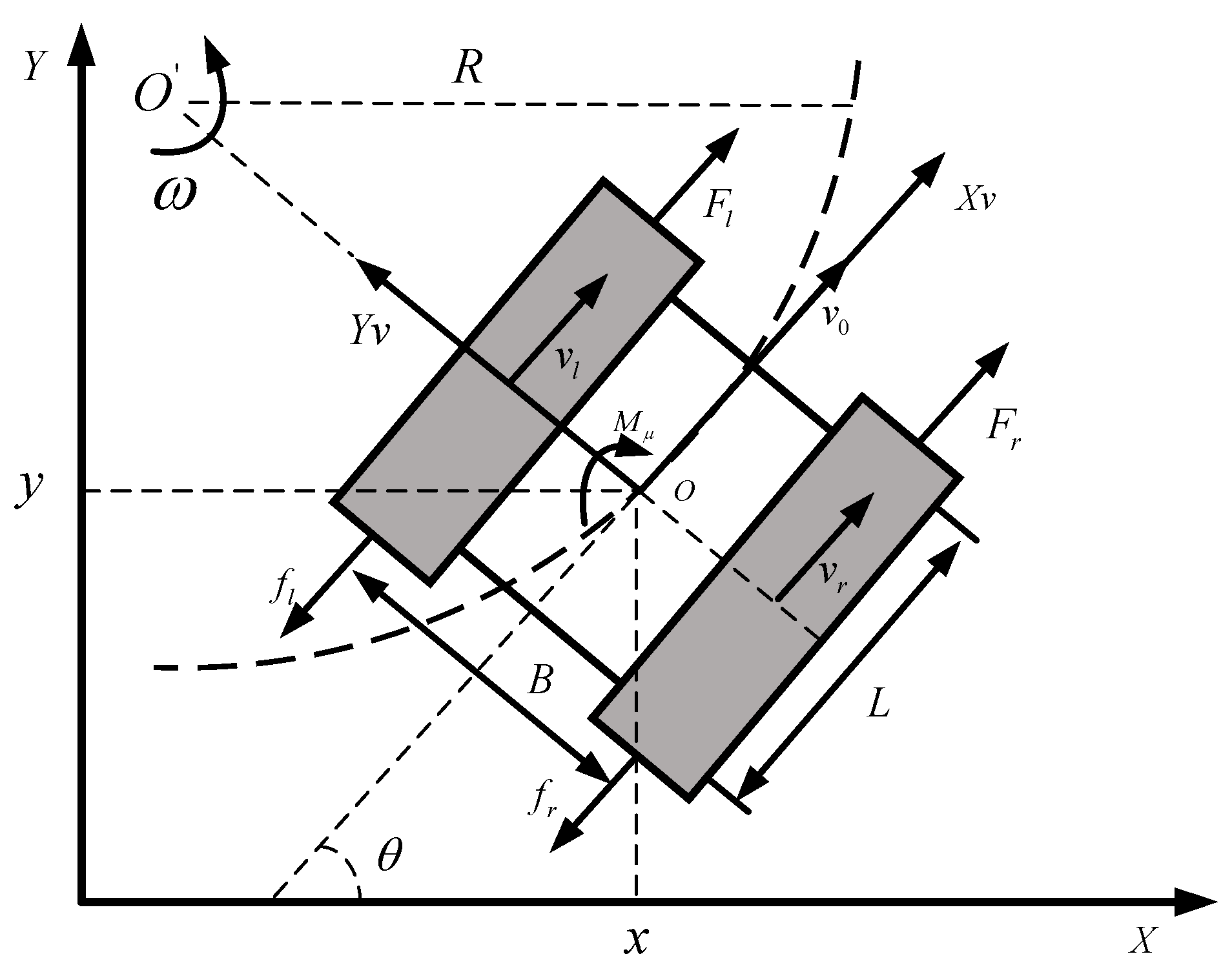
2. Dynamic Model of a Tracked Unmanned Vehicle

A vehicle kinematics model is a mathematical model that describes the laws of motion of a vehicle. It usually includes parameters such as the position, velocity, acceleration, and steering angle of the vehicle, as well as equations describing its laws of motion. By building a vehicle model, simulation experiments can be conducted to verify the effectiveness of the path tracking algorithm. By simulating the vehicle’s motion behavior in different scenarios, the performance of the path tracking algorithm can be evaluated and parameter-tuning and optimization can be performed. Common vehicle models are the kinematic and dynamic models. The kinematic model describes the vehicle motion state by calculating the acceleration, velocity, and position of the vehicle. And the dynamics model considers the force, mass, inertia, and other characteristics when describing the vehicle’s motion. Therefore, in this paper, tracked vehicle dynamics models are introduced.

The main body of the tracked unmanned vehicle chassis is rectangular in shape and carries the weight and equipment of the entire system. The tracks on both sides are the key moving parts, consisting of multiple track-plates supported and driven by drive wheels, load wheels, and carrier wheels. The tracks on both sides of the vehicle are driven by independent motors. When the vehicle is traveling in a straight line, both motors output the same rotational speed and torque, the tracks advance at the same linear speed, and the vehicle maintains a straight-line motion. When steering, differential steering is realized by controlling the different speeds of the motors on both sides. The torque output from the motors overcomes the friction resistance between the track and the ground, the friction inside the track, and the inertia resistance when the vehicle is steering, providing the power base for steering.

A steering schematic of a tracked vehicle is shown in Figure 1.

Tracked vehicles rely on two electric motors to overcome rolling resistance and steering resistance. The vehicle dynamics model is represented as follows:

$$\left\{\begin{array}{l}m\stackrel{·}{v_0}=F_1+F_r-f_l-f_r-C_{d}A{v}_0^2/21.15\\ I_z\stackrel{·}{\omega }=\left(F_r-F_l\right)B/2+\left(f_l-f_r\right)B/2-M_{\mu }\\ f_l=f_r=0.5fmg\\ M_{\mu }=0.25\mu mgl\\ v_l=v_0-0.5\omega B\\ v_r=v_0+0.5\omega B\end{array}\right.$$

(1)

where $F_l$ and $F_r$ are the driving forces of the left and right motors, respectively. $f_l$ and $f_r$ denote the corresponding track rolling resistance. $M_{\mu }$ denotes the steering resistance movement. $C_d$ and A represent the air resistance coefficient and the frontal area of the vehicle, respectively, and $v_0$ is the velocity of the vehicle at the center point. In addition, $B$ is the tread surface of the vehicle. $I_z$ and m represent the yaw moment of inertia and mass of the vehicle, respectively. $f$ is the coefficient of radial rolling resistance of the vehicle, $\mu$ denotes the coefficient of lateral resistance, and g is the acceleration of gravity. Based on the empirical results, $\mu$ is calculated by the following formula:

$$\mu ={\mu }_{\max }/\left(0.925+0.075R/B\right)$$

(2)

where ${\mu }_{max}$ is the maximum value of the lateral drag coefficient, determined by the terrain characteristics. The turning radius R is calculated as follows, where track slip is neglected:

$$R={\displaystyle \frac{B}{2}}{\displaystyle \frac{v_r+v_l}{v_r-v_l}}={\displaystyle \frac{v_0}{\omega }}$$

(3)

Since the drive of the vehicle is provided by two motors, the drive can be expressed as follows:

$$\left\{\begin{array}{l}{F}_l=T_l{i}_0{\eta }_T/r\\ F_r=T_r{i}_0{\eta }_T/r\end{array}\right.$$

(4)

where $T_r$ is the right motor torque. $T_l$ is the left motor torque. $i_0$ denotes the lateral transmission ratio. $r$ is the radius of the drive wheel. ${\eta }_T$ denotes the efficiency from the drive motor shaft to the track, calculated as follows:

$${\eta }_T=0.95-0.003v_0$$

(5)

The parameters of the tracked vehicle dynamics model, adopted from reference [35] and shown in

Table 1. Crawler vehicle dynamics and model parameters.

Parameter	Physical Meaning	Value
m	Curb weigh	1200 kg
g	Gravitational acceleration	9.8 kg/m2
f	Rolling resistance coefficient	0.05
r	Driving wheel radius	0.25 m
i0	Side driving ratio	8.21
Iz	yaw moment of inertial	1500
L	Contact length of the track on the ground	1.6 m
${\mu }_{max}$	Maximum coefficient of lateral resistance	0.49
CD	Air resistance coefficient	0.6
A	Windward area of the vehicle	1.12 m2

, were validated in the same reference to demonstrate acceptable accuracy, which justifies its application in this study.

It is also necessary to calculate the position of the vehicle in the geodetic coordinate system, which is crucial for path tracking. The counterclockwise direction of the vehicle rotation is positive, and the position of the vehicle should satisfy the following differential equation:

$$\left\{\begin{array}{l}\stackrel{·}{x}\left(t\right)=v_0\cos \theta \\ \stackrel{·}{y}\left(t\right)=v_0\sin \theta \\ \stackrel{·}{\theta }\left(t\right)=\omega \end{array}\right.$$

(6)

where $x\left(t\right)$ and $y\left(t\right)$ are the displacements of the tracked vehicle in the x—direction and y—direction respectively in the geodetic coordinate system, $\theta \left(t\right)$ is the relative rotation angle between the vehicle coordinate system and the geodetic coordinate system.

3. Path Tracking Control Strategy for Tracked Unmanned Vehicles

3.1. Hierarchical Control Strategy for Path Tracking of a Tracked Unmanned Vehicle

In order to improve the path tracking accuracy of tracked unmanned vehicles, this paper proposes a path tracking hierarchical control strategy based on DDPG-PP, as shown in Figure 2.

As shown in Figure 2, in order to realize the high-precision path tracking of tracked unmanned vehicles, this paper constructs a layered control architecture based on DDPG-PP. The upper controller is designed based on the DDPG algorithm, and, using the pre-trained reinforcement learning model, with the goal of minimizing the path tracking error, it senses the vehicle state information in real-time and dynamically calculates the optimal look-ahead distance. The lower controller adopts the PP method and calculates the torque required for the steering of the tracked unmanned vehicle based on the look-ahead distance output from the upper layer so as to realize the precise control of the steering of the vehicle and ultimately ensure that the unmanned vehicle can track the planned path stably.

3.2. Tracked Unmanned Vehicle Path Tracking Upper Controller Design

The main purpose of the upper controller is to calculate the look-ahead distance according to the state of the tracked unmanned vehicle system. Considering the traditional look-ahead distance calculation method, due to the relationship between the influencing factors and the look-ahead distance, it is difficult to be accurately portrayed by mathematical expressions, which leads to the lack of reasonableness of the look-ahead distance selection, and the vehicle and the path connection are not sufficiently considered during the selection, resulting in the poor adaptability of the model. This paper adopts the DDPG algorithm to design an intelligent and adaptive look-ahead distance selection method. In this paper, the DDPG algorithm is used to design the upper controller to realize the intelligent and adaptive selection of the look-ahead distance.

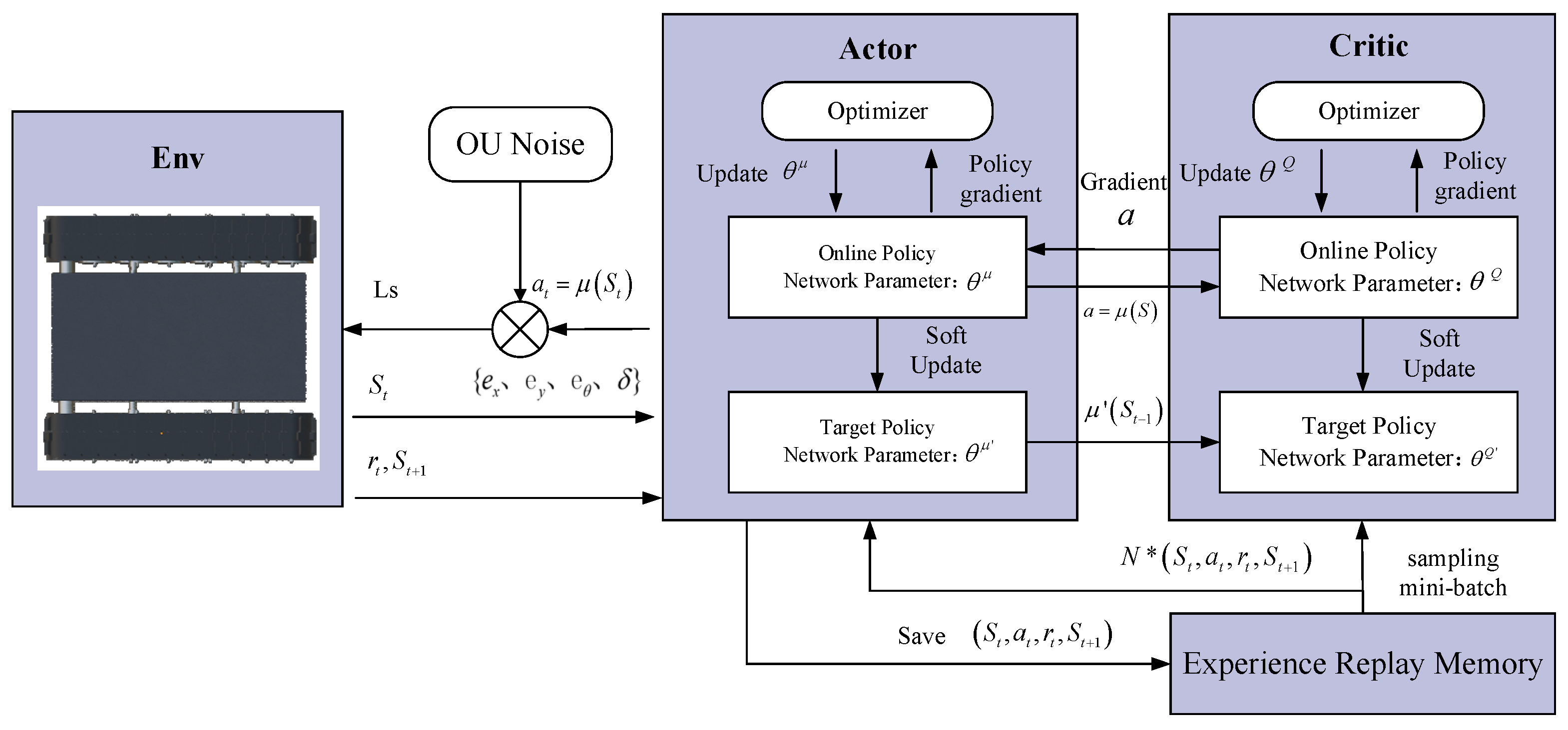
3.2.1. Principle of the DDPG Algorithm

DDPG is a reinforcement learning method that focuses on allowing for an intelligent body to learn autonomously in a specific environment by continuously interacting with the environment and taking a series of actions to maximize the cumulative reward. In reinforcement learning, the intelligent body chooses an action based on the current state by sensing the state of the environment, and the environment gives a new state as well as a reward value based on the intelligent body’s action. The goal of the intelligent body is to learn a strategy, i.e., a mapping from states to actions, that allows for as much cumulative reward as possible over a long period of interaction.

In the field of reinforcement learning, Markov Decision Process (MDP) is a widely used mathematical framework for modeling the decision process and formulating optimal strategies. The MDP consists of states, actions, state transfer probabilities, and rewards to describe a decision problem in which an agent takes actions to maximize the cumulative rewards in an environment. By solving the MDP, the optimal strategy, i.e., the best action to take in each state to maximize the long-term cumulative reward, can be found. The basic features of the MDP are shown in Equation (7).

$$P\left(s^{\prime },r|s,a\right)=\mathrm{Pr}\left\{S_{t+1}=s^{\prime },R_{t+1}=r|S_t=s,A_t=a\right\}$$

(7)

where the state space (S) contains all possible states; the action space (A) contains all possible actions that the intelligent body may take in each state; the transfer function (P) is the probability of transferring from one state to another according to the decision of a particular action; and the reward function (R) is the reward that the intelligent body obtains after taking action in a particular state. Traditional MDP frameworks are usually difficult to deal with in high-dimensional, continuous action spaces. The DDPG algorithm uses the actor-critic algorithm as its basic framework, employs deep neural networks as an approximation of the policy network and the action–value function, and uses the stochastic gradient method to train the parameters in the policy network and the value network models. The DDPG algorithm architecture uses a dual neural network architecture for both the strategy function and the value function, which makes the algorithm’s learning process more stable and accelerates the speed of convergence. At the same time, the algorithm introduces an experience playback mechanism, where the experience data samples generated from the interaction between the actor and the environment are stored in the experience pool, and the batch data samples are extracted for training, which removes the correlation and dependence of the samples and makes the algorithm easier to converge.

The output of the actor network is a deterministic action defined as $a=\mu (s,a|{\theta }^{\mu })$. μ is an estimation network that generates real-time actions, where ${\theta }^{\mu }$ is a parameter. The estimation network outputs action a based on the current state $s_t$ and interacts with the environment to generate the next state $s_{t+1}$ and reward $r_{t+1}$. The critic network is designed to fit a value function $Q\left(s,a|{\theta }^Q\right)$, which provides feedback to the actor network to judge the merit of the current action. The pseudo-code for DDPG is shown in Algorithm 1.

Algorithm 1 DDPG algorithm

${\theta }^Q$ and ${\theta }^{\mu }$ randomly initialize Critic networks $Q\left(s,a|{\theta }^Q\right)$ and Actor networks $\mu (s,{\theta }^{\mu })$ ${\theta }^{Q\prime }\leftarrow {\theta }^Q,{\theta }^{\mu \prime }\leftarrow {\theta }^{\mu }$ initialize target network weights $Q\prime$ and $\mu \prime$ Initialize the experience playback area R for episode = 1, M do:         Action exploration, random noise N initialization         Obtaining the initial observation state $s_t$         for t = 1, T do:                                           $a_t=\mu \left(s_t|{\theta }^{\mu }\right)+N_t$         Execute an action $a_t$, achieve $r_t$ and environmental state $s_{t+1}$, data $(s_t,a_t,r_t,s_{t+1})$ save to R.         Randomly sample a multidimensional array $(s_t,a_t,r_t,s_{t+1})$ of batch number values N from R                                               $y_t=r_t+\gamma Q^{\prime }\left(s_{t+1},{\mu }^{\prime }\left(s_{t+1}|{\theta }^{{\mu }^{\prime }}\right)|{\theta }^{Q^{\prime }}\right)$         Minimize the loss function L to update the Critic network:                                            $L={\displaystyle \frac{1}{N}}{\displaystyle {\sum }_i{\left(y_t-Q\left(s_t,a_t|{\theta }^Q\right)\right)}^2}$         The Actor policy network is updated by policy gradient:                                            ${\nabla }_{{\theta }^{\mu }}J\left({\theta }^{\mu }\right)\cong {\displaystyle \frac{1}{N}}{\displaystyle {\sum }_i{\nabla }_{{\theta }^{\mu }}\mu \left(s_t|{\theta }^{\mu }\right)}{\nabla }_{a}Q\left(s_t,a|{\theta }^Q\right){|}_{a=\mu \left(s_t\right)}$         Update the target network:                                            $\begin{array}{l}{\theta }^{Q^{\prime }}\leftarrow \tau {\theta }^Q+\left(1-\tau \right){\theta }^{Q^{\prime }}\\ {\theta }^{{\mu }^{\prime }}\leftarrow \tau {\theta }^{\mu }+\left(1-\tau \right){\theta }^{{\mu }^{\prime }}\end{array}$         End For End For

3.2.2. Upper Controller Design Based on DDPG

The DDPG-based path tracking upper controller consists of four networks, an OU noise module, a reward value calculation module, and an experience pool. The four networks are the actor network, commenter network, target actor network and target commenter network. The role of the OU noise module is to increase the exploration of strategies. The reward value calculation module can calculate the reward value for network learning based on the current state. The experience pool is designed to increase the utilization of data, and the overall framework is shown in Figure 3.

The DDPG is designed to handle continuous action space, enabling it to meticulously adjust and optimize the look-ahead distance to provide smoother control effects, thus improving the problem of poor tracking due to the difficulty in adjusting the look-ahead distance in PP algorithms. Its state, action, and reward functions are defined as follows.

The selection of an appropriate state space is crucial for the convergence of the reinforcement learning algorithm. The selected state information should be related to the motion state of the tracked vehicle as well as the path information.

$$s_t=\left\{e_x,e_y,e_{\theta },\delta \right\}$$

(8)

where $e_x$ denotes the longitudinal error between the tracked vehicle and the look-ahead point, $e_y$ denotes the lateral error between the tracked vehicle and the look-ahead point, $e_{\theta }$ denotes the yaw error between the tracked vehicle and the look-ahead point, and $\delta$ denotes the ratio of the speeds between the left and right tracks, which is used to characterize the path curvature information.

The action denoted $a=\mu (s,a|{\theta }^{\mu })$ is expressed as the look-ahead distance Ls and acts on the PP algorithm.

The reward function is designed to penalize the tracked vehicle when it deviates from the path, as shown in Equation (9).

$$r\left(t\right)=-e_y^2$$

(9)

where $e_y$ denotes the lateral error between the tracked vehicle and the look-ahead point; this design ensures that the lateral error is penalized and that the penalty is higher when the lateral error is larger and smaller when the lateral error is smaller.

The network structure consists of two actor networks and two commentator networks. Both the actor and commenter neural networks are composed of two hidden layers. Each layer is equipped with a Rectified Linear Unit (ReLU) activation function with 256 neurons in both hidden layers. The action undergoes a tanh transformation to limit its range. In the evaluation network, actions and states are concatenated to form an input. For the optimization of the neural network, the Adam optimizer is used with a small batch data size of 256. Subsequently, five separate training sessions are performed to evaluate the effectiveness and stability of the algorithm. Each training utilizes a different random seed to control the path generation parameters. This approach ensures the reproducibility of the experiments. The hyperparameters are summarized in

Table 2. Hyperparameters of both the actor and critic networks for path following.

Description	Value
Number of hidden layers	2
Number of neurons per layers	256
Activation function	ReLU
Optimizer	Adam
Learning rate	5 × 10−4
Minibatch size	256

.

The training environment consists of a robot dynamics model together with a reference path. Given the complexity of real-world application scenarios, it is particularly critical to ensure that the intelligent body strategies are adaptable to diverse challenges. Such adaptability can enhance the decision-making ability of the strategy in generalized scenarios and effectively circumvent the performance degradation problem caused by over-fitting specific path features. In order to enhance the generalization ability of the model, this paper adopts a stochastic path generation algorithm [36] which introduces dynamically variable training trajectories to drive the intelligent body to learn under diverse environmental conditions so as to strengthen its robustness in dealing with complex scenarios. The Stochastic Path Generate Algorithm is shown in Algorithm 2.

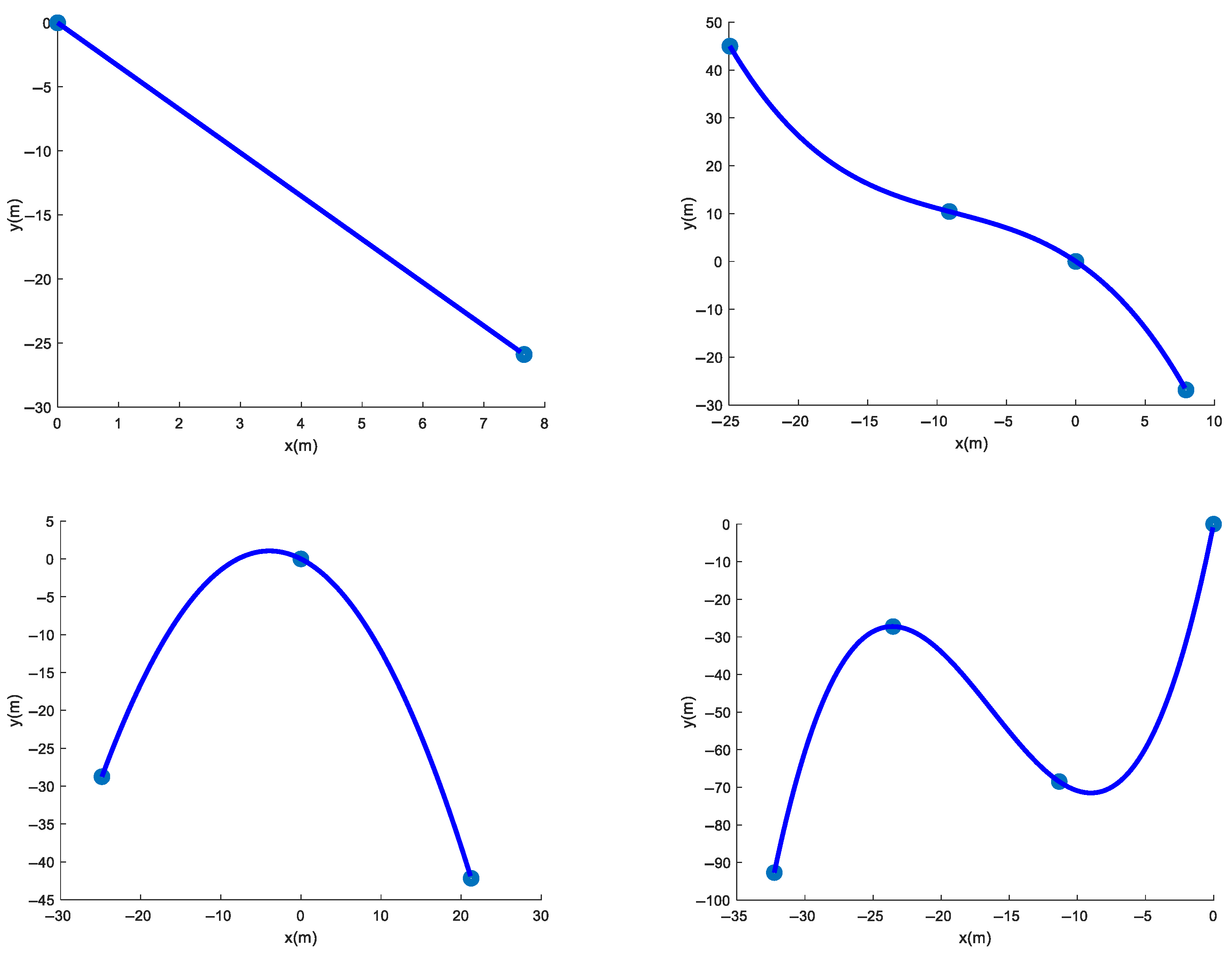
Algorithm 2 Stochastic Path Generate Algorithm

Generated waypoint counter n←1, starting waypoint p1←[0,0], Number of path waypoints $N_{\omega }\in \mathbb{N}$, Range of length between waypoints $[L_{min},L_{max}]\in {\mathbb{R}}^{+}$ While $n\le N_{\omega }$ do        Sample $L_{\omega }$ from $randi\left(L_{min},L_{max}\right)$        Sample ${\theta }_{\omega }$ from $randi\left(\mathrm{0,2}\pi \right)$        New $\mathrm{waypoint} {\mathrm{P}}_{\mathrm{n}+1}\leftarrow {\mathrm{P}}_{\mathrm{n}}+L_{\omega }{\left[\mathrm{c}\mathrm{o}\mathrm{s}\right({\theta }_{\omega }),\mathrm{s}\mathrm{i}\mathrm{n}({\theta }_{\omega }\left)\right]}^T$        n←n + 1 End while Create parameterized path $P_T\left(\omega \right)={[x_T\left(\omega \right),y_T\left(\omega \right)]}^T$ using Cubic Spline Interpolator

In this paper, $N_{\omega }$= U (2, 6), $L_{min}$ = 25, $L_{max}$ = 50. Figure 4 shows some of the paths randomly generated using the algorithm.

At each environment reset, the random seed is reset to control the path generation parameters and compute the path data, the tracked unmanned vehicle is forced to be placed at the path start position and heading, and, at the same time, the vehicle state is zeroed out, thus eliminating the residual influence of the vehicle state at the end of the previous round of training, which ensures the independence and consistency of the training data for better generalization to various real-world scenarios.

3.3. Tracked Unmanned Vehicle Path Tracking Lower Controller Design

The core function of the lower controller is to accurately calculate the steering torque required for the tracked unmanned vehicle to realize path tracking based on the look-ahead distance output from the upper controller. In this design, the PP algorithm is adopted to determine the required track speed for steering and the steering torque based on the look-ahead distance output from the upper layer, forming a control architecture of “speed planning–torque calculation” to achieve precise control of the torque required for steering.

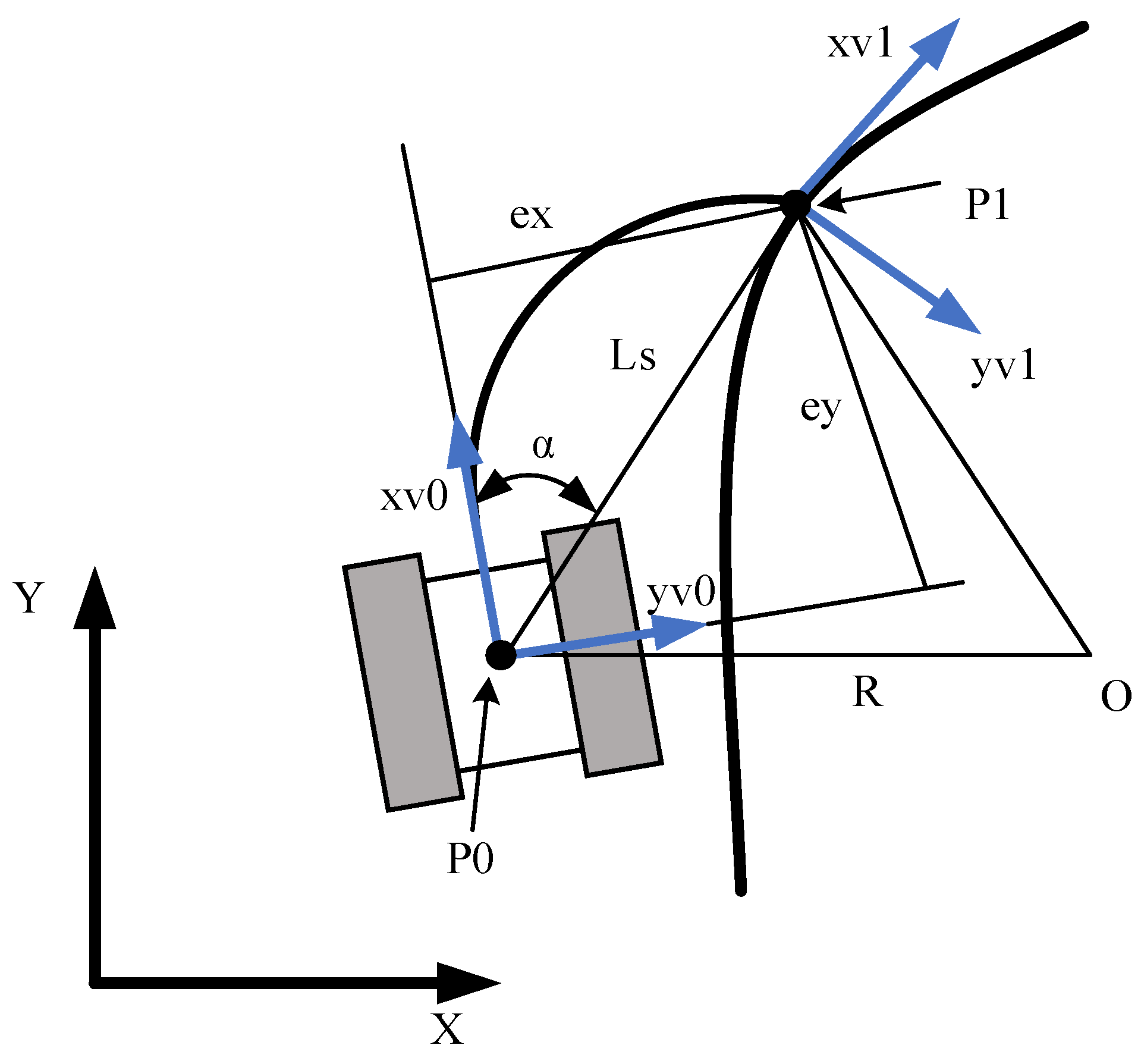
3.3.1. Principles of the PP Algorithm

The PP algorithm, proposed by R. Wallace in 1985, is a traditional geometric path tracking method. The PP algorithm was originally applied to front-wheel-steering vehicles, which utilizes the geometric relationship between the look-ahead point and the vehicle to calculate the steering angle and thus realize the lateral control of the vehicle. The application of the PP algorithm to tracked vehicles is different from that of front-wheel-steering vehicles, and the schematic diagram of the PP algorithm is shown in Figure 5.

$P0(X_0,Y_0,{\theta }_0)$ is the current position of the tracked vehicle. Take P0 as the center of the circle and the look-ahead distance Ls as the radius to make a circle intersecting the path at the look-ahead point $P1(X_1,Y_1,{\theta }_1)$. Make an extension line P0O at point P0 along the direction perpendicular to the current heading, and, at the same time, make a vertical line P1O at point P1 along the vertical direction of its heading and intersect with P0O at point O. Point O is the current vehicle rotation center. Take the distance R from P1O as the radius and make an arc through P0 and P1, which is the expected traveling path.

According to the cosine theorem, the following equation can be obtained:

$${\displaystyle \frac{Ls}{\sin \left(2\alpha \right)}}={\displaystyle \frac{R}{\sin \left(\frac{\pi }{2}-\alpha \right)}}$$

(10)

The expression of $R$ can be obtained as

$$R={\displaystyle \frac{Ls}{2\sin \alpha }}$$

(11)

In the formula, $\alpha$ is the angle between the vehicle heading and the preview point at this time, and the calculation formula is

$$\sin \alpha ={\displaystyle \frac{e_y}{Ls}}$$

(12)

where $e_y$ is the lateral error under the vehicle body coordinate system on the tracked vehicle forward path. The relationship between the error under the geodetic coordinate system, and the vehicle body coordinate system is

$$\left[\begin{array}{l}{e}_x\\ e_y\\ e_{\theta }\end{array}\right]=\left[\begin{array}{ccc}\begin{array}{l}\cos \theta \\ -\sin \theta \\ 0\end{array}& \begin{array}{l}\sin \theta \\ \cos \theta \\ 0\end{array}& \begin{array}{l}0\\ 0\\ 1\end{array}\end{array}\right]\left[\begin{array}{l}{X}_r-X\\ Y_r-Y\\ {\theta }_r-\theta \end{array}\right]$$

(13)

where ${\left[X_r,Y_r,{\theta }_r\right]}^T$ is the look-ahead point, and its calculation process is satisfied with the pseudocode, as shown in Algorithm 3.

Algorithm 3 Look-Ahead Point Generate Algorithm

$\mathrm{calculate} \mathrm{the} \mathrm{distance} \mathrm{sequence} \mathrm{between} \mathrm{the} \mathrm{path} \mathrm{and} \mathrm{the} \mathrm{vehicle} dist,$ $\mathrm{Initialize} \mathrm{parameters} L{s}_{step}=0, idx=\mathrm{argmin}\left(dist\right)$ $\mathbf{if} Ls<\mathrm{m}\mathrm{i}\mathrm{n}\left(dist\right)$    $\mathrm{Generate} \mathrm{Ls} Ls=\mathrm{m}\mathrm{i}\mathrm{n}\left(dist\right)$ else    While $L{s}_{step}<Ls$       Generate $L{s}_{step}=dist\left[idx\right]$       Generate $idx=idx+1$    End while    Generate $Ls=Ls\_step$    Generate look-ahead point ${\left[X_r,Y_r,{\theta }_r\right]}^T=curve\left[idx\right]$ End if

From Equation (11) and Equation (12), we obtain

$$R={\displaystyle \frac{L{s}^2}{2e_y}}$$

(14)

Equation (14) can be rewritten as

$$k={\displaystyle \frac{2e_y}{L{s}^2}}$$

(15)

From Equation (14), it can be seen that the PP algorithm is equivalent to a proportional control based on the error $e_y$; the control system is $2/{Ls}^2$, and its output is the steering radius of the vehicle motion.

From Equation (3) and Equation (15), we can obtain

$$\delta ={\displaystyle \frac{v_r}{v_l}}={\displaystyle \frac{2+Bk}{2-Bk}}$$

(16)

The velocities of the tracks on both sides required for path tracking are finally obtained.

3.3.2. PP-Based Lower Controller Design

Based on the PP lower controller, the PP algorithm firstly calculates the ratio of the left and right track speeds required for steering based on the look-ahead distance. In order to obtain the exact left and right track speeds, this paper adopts the differential algorithm to calculate the required speed for steering, and the specific calculation formula is shown in the following equation:

$$\left\{\begin{array}{l}{v}_l={\displaystyle \frac{2v}{1+\delta }}\\ v_r={\displaystyle \frac{2v\delta }{1+\delta }}\end{array}\right.$$

(17)

where $v_l$ and $v_r$ are the left track speed and the right track speed, respectively; $v$ is the desired speed of the tracked vehicle; and $\delta$ is the ratio of the left and right track speeds.

In this design, a PID controller is used to realize the tracking of tracked vehicle to the speed command of PP algorithm. PID control is proportional–integral–differential control. It is a widely used control algorithm in engineering applications. The control signal for PID can be generated using Equation (18):

$$u\left(t\right)=K_{p}e\left(t\right)+K_i{\displaystyle \int e\left(t\right)dt+K_d\frac{de\left(t\right)}{dt}}$$

(18)

where $K_P$, $K_i$, and $K_d$ are the parameters to be tuned by this controller and $e\left(t\right)$ is the error between the actual track speed and the desired track speed. $\mu \left(t\right)$ is the throttle opening for realizing the regulation of the output torque. The output torque is calculated as

$$\left\{\begin{array}{l}T={\displaystyle \frac{u\left(t\right)}{Acc}}f\left(n\right)\\ n={\displaystyle \frac{30v{i}_o}{\mathrm{r}\pi }}\end{array}\right.$$

(19)

where $Acc$ is the maximum throttle opening and f is a look-up table function of the maximum output torque at speed $n$.

In a PID controller, the proportional term $K_P$ provides an output that is proportional to the error between the desired and actual values. This term responds quickly to the error to reduce it, but may not be able to eliminate it completely. The integral term $K_i$ accumulates error over time and provides an output proportional to the integral of the error. This term helps to eliminate the steady-state error and ensures that the system achieves the desired value. The differential term $K_d$ provides an output proportional to the rate of change of the error. This term predicts the trend of the system and responds to rapidly changing errors, helping to improve the stability and responsiveness of the system.

3.4. LQR Controller Designed for Comparison Experiments

In the research of path tracking control strategies for tracked unmanned vehicles, reasonable comparative experiments are an important means to evaluate the performance advantages and disadvantages of different control algorithms. In this section, the LQR controller is introduced for comparative experiments. By elaborating its design principle, parameter adjustment, and performance verification, it provides a new perspective and strong support for the in-depth study of the path tracking control strategies of tracked unmanned vehicles.

3.4.1. Principle of LQR

The LQR controller belongs to the control technique obtained by constructing the state space equation of the controlled object, and the linear state space equation of the controlled system is shown as follows:

$$\left\{\begin{array}{l}\dot{x}\left(t\right)=A\left(t\right)x\left(t\right)+B\left(t\right)u\left(t\right),x\left(t\right)=x_0\\ y=C\left(t\right)x\left(t\right)\end{array}\right.$$

(20)

Define the quadratic performance index with respect to the state vector and the control vector as

$$J={\displaystyle {\int }_{t_0}^{t_f}\left[x^T\left(t\right)Qx\left(t\right)+u^T\left(t\right)Ru\left(t\right)\right]}$$

(21)

where $Q$ is an n × n-dimensional semipositive (or positive definite) symmetric matrix, $R$ is an m × m-dimensional positive definite matrix, and $t_f$ tf is the time at which the system is running.

The feedback matrix $K$ in the optimal control law requires solving the Riccati matrix differential equation, which is described by the Riccati equation as follows:

$$A^{T}P+PA-PB{R}^{-1}{B}^{T}P+Q=0$$

(22)

where $P$ is the unknown matrix to be solved. $A$ and $B$ are the state transfer matrices and control coefficients matrices in the system state equations, and $Q$ and $R$ are the loss function weight matrices in the quadratic performance index.

Solving the $P$ matrix in the Riccati equation, the feedback matrix $K$ can be expressed as follows:

$$K=-R^{-1}{B}^{T}P$$

(23)

At this point, the optimal control law ${\mu }^{*}\left(t\right)$ is denoted by the following:

$$u^{*}\left(t\right)=-Kx\left(t\right)$$

(24)

3.4.2. Design of LQR Based Path Tracking Controller for Tracked Unmanned Vehicles

As shown in Figure 1, neglecting the lateral deflection angle, the lateral velocity of the crawler robot in the local coordinate system is zero and the longitudinal velocity is $v$. The linear velocities of the crawler robot in the direction of the $X$ and $Y$ axes in the global coordinate system are discretized under the local coordinate system, which can be expressed as follows:

$$\left\{\begin{array}{l}\dot{X}\cos \theta +\dot{Y}\sin \theta =v\\ \dot{Y}\cos \theta -\dot{X}\sin \theta =0\end{array}\right.$$

(25)

Differentiating Equation (25), we obtain

$${\dot{e}}_x=({\dot{X}}_r-\dot{X})\cos \theta -(X_r-X)\dot{\theta }\sin \theta +({\dot{Y}}_r-\dot{Y})\sin \theta +(Y_r-Y)\dot{\theta }\cos \theta$$

(26)

$${\dot{e}}_y=(\dot{X}-{\dot{X}}_r)\sin \theta -(X_r-X)\dot{\theta }\cos \theta +({\dot{Y}}_r-\dot{Y})\cos \theta +(Y_r-Y)\dot{\theta }\sin \theta$$

(27)

Using Equation (25) to simplify Equations (26) and (27), the differential equation for the position error is obtained:

$$\left(\begin{array}{l}{\dot{e}}_x\\ {\dot{e}}_y\\ {\dot{e}}_{\theta }\end{array}\right)=\left(\begin{array}{l}{e}_y\omega -v+v_r\cos e_{\theta }\\ -\omega e_x+v_r\sin e_{\theta }\\ v_r\rho -w\end{array}\right)$$

(28)

When the crawler robot enters the steady state following state, at this time, $e_{\theta }\approx 0$, $cos{e}_{\theta }=1$, $sin{e}_{\theta }=e_{\theta }$. Further simplification of Equation (28) yields the differential equation of the position error of the crawler robot, as shown in Equation (29):

$$\left(\begin{array}{l}{\dot{e}}_x\\ {\dot{e}}_y\\ {\dot{e}}_{\theta }\end{array}\right)=\left(\begin{array}{l}{e}_y\omega -v+v_r\\ -\omega e_x+v_r{e}_{\theta }\\ v_r\rho -w\end{array}\right)$$

(29)

The lateral deviation $e_y$ and the heading angular deviation $e_{\theta }$ in the error differential equation are chosen as the state vectors of the controlled object, and the rotation angular velocity $\omega$ is used as the input action of the controlled system. The linear system of tracked mobile robot can be expressed as follows:

$$\left\{\begin{array}{l}\dot{x}\left(t\right)=\left[\begin{array}{c}\begin{array}{cc}0& v_r\end{array}\\ \begin{array}{cc}0& 0\end{array}\end{array}\right]x\left(t\right)+\left[\begin{array}{l}-e_x\\ -1\end{array}\right]u\left(t\right)\left[\begin{array}{l}0\\ v_r\end{array}\right]\rho \\ y\left(t\right)=\left[\begin{array}{l}\begin{array}{cc}1& 0\end{array}\\ \begin{array}{cc}0& 1\end{array}\end{array}\right]x\left(t\right)\end{array}\right.$$

(30)

where $x\left(t\right)=\left[\begin{array}{c}{e}_y\\ e_{\theta }\end{array}\right]$,$u\left(t\right)=\omega$,$A=\left[\begin{array}{c}\begin{array}{cc}0& v_r\end{array}\\ \begin{array}{cc}0& 0\end{array}\end{array}\right]$, $B=\left[\begin{array}{c}-e_x\\ -1\end{array}\right]$.

The form of the $Q$, $R$ matrix can be expressed as

$$Q\left[\begin{array}{l}q1\begin{array}{cc}& 0\end{array}\\ \begin{array}{cc}0& q2\end{array}\end{array}\right],R=r$$

(31)

where $q1$ = 8.5684 and $q2$ = 1.4256 denote the weighting coefficients on the lateral deviation $e_y$ and the heading angle deviation $e_{\theta }$, respectively. According to modern control theory, the larger the weighting coefficient, the more important the state variable is in the performance function; $r$ = 0.1 denotes the weighting coefficient on the rotational angular velocity $\omega$, and the larger the value, the stronger the control constraints.

Solving the Riccati equation yields the feedback matrix $K$. The optimal control law ${\mu }^{*}\left(t\right)$ of the LQR path-following controller is denoted by the following:

$$u^{*}\left(t\right)=-Kx\left(t\right)=-k_1{e}_y-k_2{e}_{\theta }$$

(32)

4. Simulation and Verification

4.1. Result of Path Tracking Control Strategy Training

The model training environment is configured as follows: Intel(R) Core (TM) i7-14650 HX processor with NVIDIA GeForce RTX 4060 Laptop GPU and 16 GB RAM, all installed in a Lenovo Y7000P laptop (manufactured by Lenovo in Hefei, China) to meet the demand of complex computing. The operating system is Windows 11. The training environment was built using Simulink, the model was trained according to the hyperparameters shown in Table 2, and the reward curves were obtained as shown in Figure 6.

The curves in Figure 6 show the average number of steps and the average reward value of the DDPG algorithm during each iteration. It can be seen that the number of steps and the reward value in the early stage of training are small and have a certain degree of randomness. In the late stage of training, both the average number of steps and the average reward value show a convergence trend, which verifies the effectiveness of the algorithm. As shown in the figure, the algorithm is in an exploratory phase at 100 steps, with a rapid increase in reward; it enters a period of rapid convergence at 100–250 steps, with a slowing down of reward growth; and it enters a period of stabilization at more than 250 steps, with a reward fluctuation of <1.5% to reach convergence.

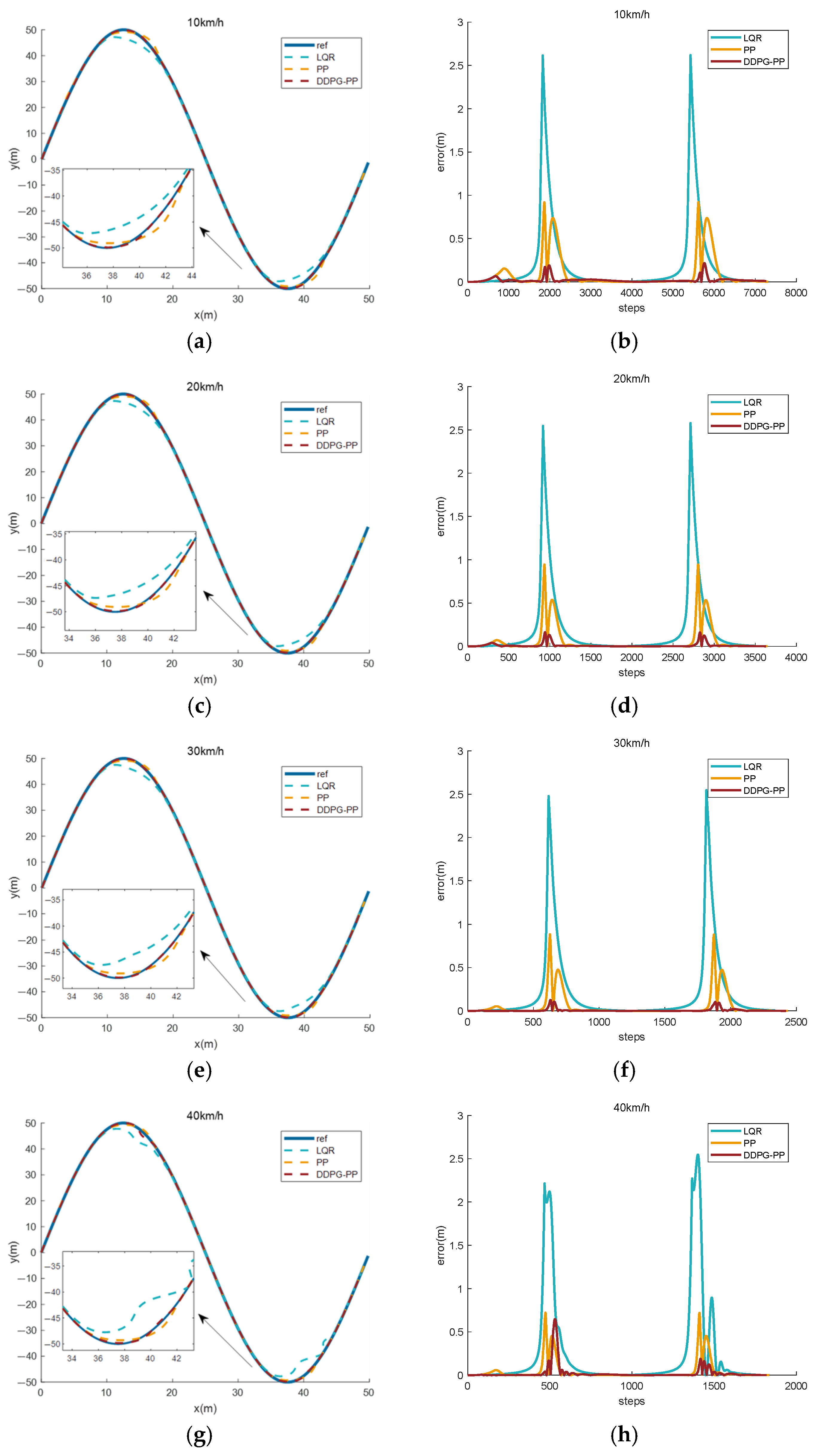
4.2. Effect of Path Tracking at Different Speeds

The path-following test path at different speeds is a sin-shaped curve that is widely used to test path tracking algorithms, as defined in Equation (33). The sin function is periodic and fluctuating, and can simulate the case of tracked vehicles undergoing curvilinear motions in the path.

$$\left\{\begin{array}{l}y=A\sin \left(\omega x+\phi \right)\\ x=\left[0,2\pi \right]\end{array}\right.$$

(33)

where $A$ is a constant that determines the height amplitude of the curve and is set to 50. $\omega$ is a constant that determines the period of the curve and takes the value of π/25. $\phi$ is a constant that determines the position of the curve and takes the value of 0. The results obtained by taking the LQR algorithm, the PP algorithm, and the DDPG-PP algorithm for tracking a given route at speeds of 10, 20, 30, and 40 km/h, respectively, are shown in Figure 7. The simulation results show that the maximum error occurs at the path bending section. The proposed algorithms all fit the path better than the comparison algorithms. The average tracking error is used as the path tracking accuracy to quantify the tracking effect, and the specific comparison results are summarized in

Table 3. Tracking results of different path tracking methods at different speeds.

Method	Velocity (km/h)
	10	20	30	40
LQR	0.2102	0.2022	0.2011	0.2498
PP	0.0905	0.0629	0.0547	0.0450
DDPG-PP	0.0215	0.0114	0.0089	0.0236

.

Table 3 presents a comparison of the tracking errors of the three path tracking methods, LQR, PP, and DDPG-PP, in the speed range of 10~40 km/h. The data show that the different algorithms exhibit significant differences in speed adaptability, error stability, and control accuracy.

The PP algorithm shows the characteristic of “error decreasing with speed” in the whole speed range: when the speed increases from 10 km/h to 40 km/h, the tracking error decreases from 0.0905 to 0.0450, which is a decrease of 50.3%. This phenomenon is directly related to the core mechanism of the PP algorithm, which dynamically adjusts the steering radius through the look-ahead distance, and the longer look-ahead distance in high-speed scenarios can effectively suppress the tracking bias caused by the change in path curvature. However, the error of PP algorithm at low speeds of 10 km/h (0.0905) is significantly higher than that of DDPG-PP (0.0215), which reflects the limitation of PP modeling in low-speed fine control. The vehicle steering radius is small in low-speed steering, and the geometric relation of the look-ahead point is less sensitive to the transverse error, which leads to the insufficient adjustment accuracy of the proportional control gain (2/Ls²).

The LQR algorithm maintains the error around 0.20 in the interval of 10~30 km/h, which shows relatively stable control performance, but the error increases abruptly to 0.2498 at 40 km/h, which is 24.2% higher than that at 30 km/h. This is due to the fact that the LQR is designed based on a linearized model, and the nonlinear characteristics of the vehicle are intensified under high-speed conditions, resulting in the amplification of the model mismatch effect.

The DDPG-PP algorithm shows a significant accuracy advantage in the range of 10~30 km/h, with errors of 0.0215, 0.0114, 0.0089, and 0.0236, respectively, which are better than the LQR algorithm and the PP algorithm. Thanks to the ability of DDPG to fit complex nonlinear mappings, the algorithm can dynamically adjust the pre-scanning strategy to achieve precise suppression of lateral errors during low-speed fine steering.

4.3. Effect of Path Tracking at Different Paths

In order to study the tracking effectiveness of the proposed algorithms on different paths, this section uses the LQR, PP, and DDPG-PP algorithms to travel on straight line paths, sin function paths, and obstacle avoidance sin function paths, respectively, at a speed of 25 km/h. The path tracking algorithms are quantitatively analyzed using average tracking error, maximum tracking error, average heading error, and maximum heading error as the evaluation indexes. The evaluation indexes are calculated as shown in Equations (34)–(37).

$$e_{\mathrm{p}}={\displaystyle \frac{1}{\mathrm{N}}}{\displaystyle \sum _{i=1}^{\mathrm{N}}\sqrt{e_{\mathrm{x}i}^2+e_{\mathrm{y}i}^2}}$$

(34)

$$e_{\mathrm{pmax}}=\max \left(\sqrt{e_{\mathrm{x}i}^2+e_{\mathrm{y}i}^2}\right)$$

(35)

$$e_{\mathsf{\theta }}={\displaystyle \frac{1}{\mathrm{N}}}{\displaystyle \sum _{i=1}^{\mathrm{N}}\left|e_{\mathsf{\theta }i}\right|}$$

(36)

$$e_{\mathsf{\theta }\max }=\max \left(\left|e_{\mathsf{\theta }i}\right|\right)$$

(37)

where $e_p$ is the average tracking error, $e_{pmax}$ is the maximum tracking error, $e_{\theta }$ is the average heading error, $e_{\theta max}$ is the maximum heading error, $e_{xi}$ is the longitudinal error, $e_{yi}$ is the lateral error, $e_{\theta i}$ is the heading error, and N is the number of samples.

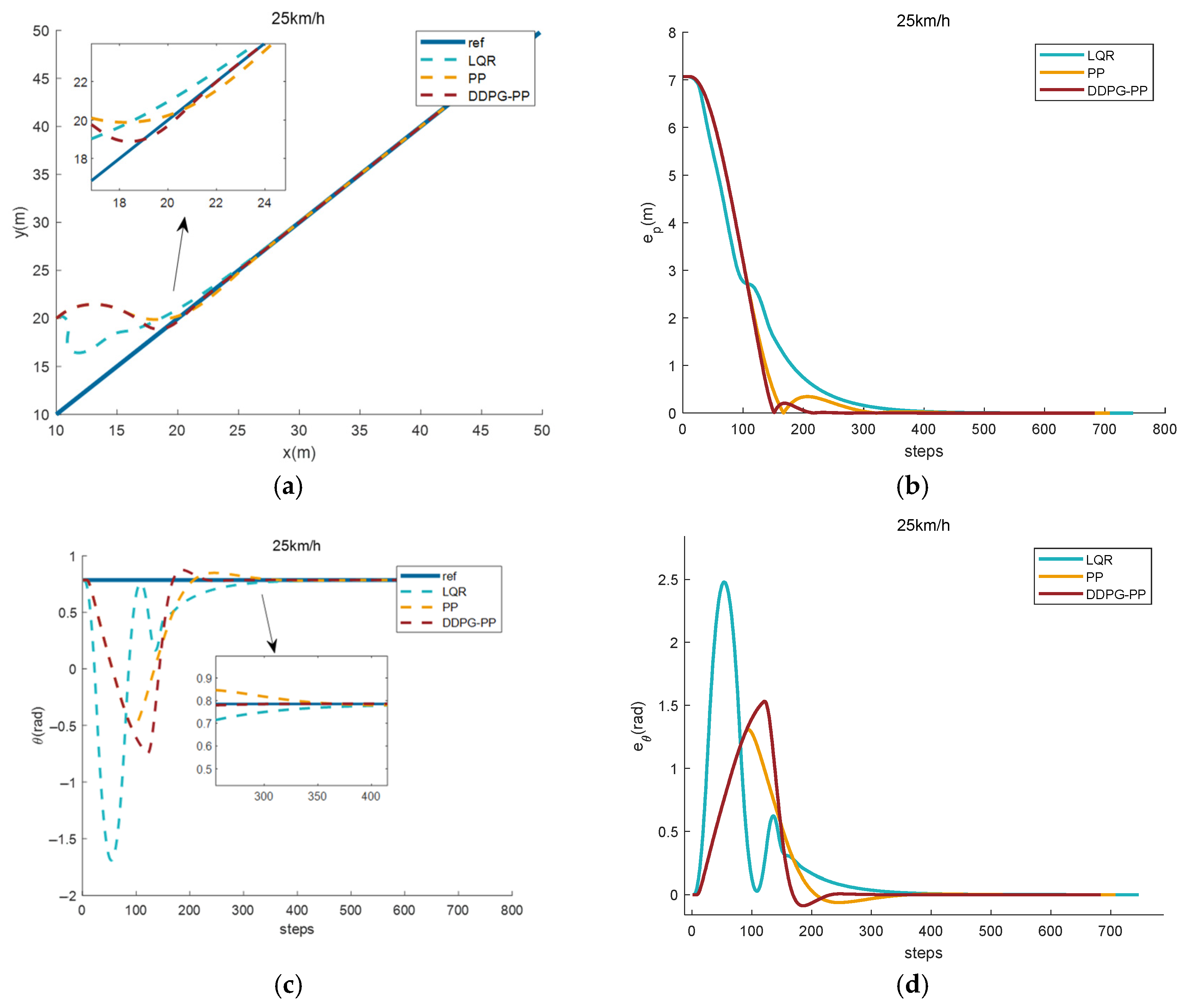
4.3.1. Effect of Path Tracking Under Straight Paths

The test path is a straight line and is used to evaluate the performance and accuracy of the system in simple situations. By setting the initial error and testing on a straight-line path, the system’s responsiveness to basic motion control can be examined. The straight-line path is the line between (10,10) and (50,50), and the tracked vehicle tracks the path starting at (10,20), as shown in Figure 8.

Simulation results show that the three methods have different responses in the initial phase of path tracking. The proposed algorithm fits the path better than the comparison algorithms. Path tracking metrics, as well as response time (time required for tracking accuracy less than 0.5 m), are used to quantify the tracking effectiveness, and the specific comparison results are summarized in

Table 4. Path tracking results of different methods under straight paths.

Method	Evaluation Indicators
	${\mathit{e}}_{\mathbf{p}}$ (m)	${\mathit{e}}_{\mathbf{p}\mathbf{m}\mathbf{a}\mathbf{x}}$ (m)	${\mathit{e}}_{\mathsf{\theta }}$ (rad)	${\mathit{e}}_{\mathsf{\theta }\mathbf{m}\mathbf{a}\mathbf{x}}$ (rad)	$\mathit{T}$ (s)
LQR	1.0032	7.0711	0.2277	2.4778	2.26
PP	0.9839	7.0711	0.1852	1.3075	1.50
DDPG-PP	0.9663	7.0711	0.2010	1.5323	1.40

.

Since all three methods can have better tracking effect on straight paths in the later stage, the values of the three methods on the average tracking error are relatively close to each other. However, the average tracking error of the DDPG-PP method is 0.9663, which is slightly lower than that of the LQR and PP methods, indicating that the DDPG-PP has an advantage in this metric. The maximum tracking error of all three methods is the initial position of the vehicle with the same value. PP method has better results in the average heading error and maximum heading error metrics, but the DDPG-PP method is not much different from it. In the response time metric T, the DDPG-PP method has a significant advantage with a value of 1.2340, which is lower than LQR and PP methods. This shows that DDPG-PP method has faster response time. Comparing the experimental results of the three methods (LQR, PP, and DDPG-PP), it can be seen that the different methods show some differences in each evaluation index. Overall, the DDPG-PP method shows superior performance in several indicators.

4.3.2. Effect of Path Tracking Under Sinusoidal Function Paths

The LQR algorithm, PP algorithm, and DDPG-PP algorithm are taken to track the given route at 25 km/h, and the route is obtained from Equation (33). The obtained results are shown in Figure 9.

The simulation results show that the maximum error occurs at the path bending section. The proposed algorithms all fit the path better than the comparison algorithms. Evaluation metrics are used to quantify the tracking effect, and the specific comparison results are summarized in

Table 5. Path tracing results of different methods under sin function paths.

Method	Evaluation Indicators
	${\mathit{e}}_{\mathbf{p}}$ (m)	${\mathit{e}}_{\mathbf{p}\mathbf{m}\mathbf{a}\mathbf{x}}$ (m)	${\mathit{e}}_{\mathsf{\theta }}$ (rad)	${\mathit{e}}_{\mathsf{\theta }\mathbf{m}\mathbf{a}\mathbf{x}}$ (rad)
LQR	0.1998	2.6011	0.0595	1.7352
PP	0.0588	0.9301	0.0298	0.5418
DDPG -PP	0.0071	0.1742	0.0064	0.1983

.

The average tracking error and the maximum tracking error of DDPG-PP are the smallest among the three methods; the value of the average tracking error is 0.0071, which is reduced by 96.44% and 87.92% with respect to the LQR method as well as the PP method, respectively. The value of the maximum tracking error is 0.1742, which is 93.30% and 81.27% lower than the LQR method and PP method, respectively. This indicates that DDPG-PP has a significant advantage in this metric and is able to track the path better. The average heading error and the maximum heading error are also the smallest among the three methods. The value of the average heading error is 0.0064, which is 89.24% and 78.52% lower than that of the LQR method and the PP method, respectively. The maximum heading error is 0.1983, which is 88.57% and 63.39% lower than the LQR and PP methods, respectively. This indicates that the DDPG-PP method is able to track the path heading better.

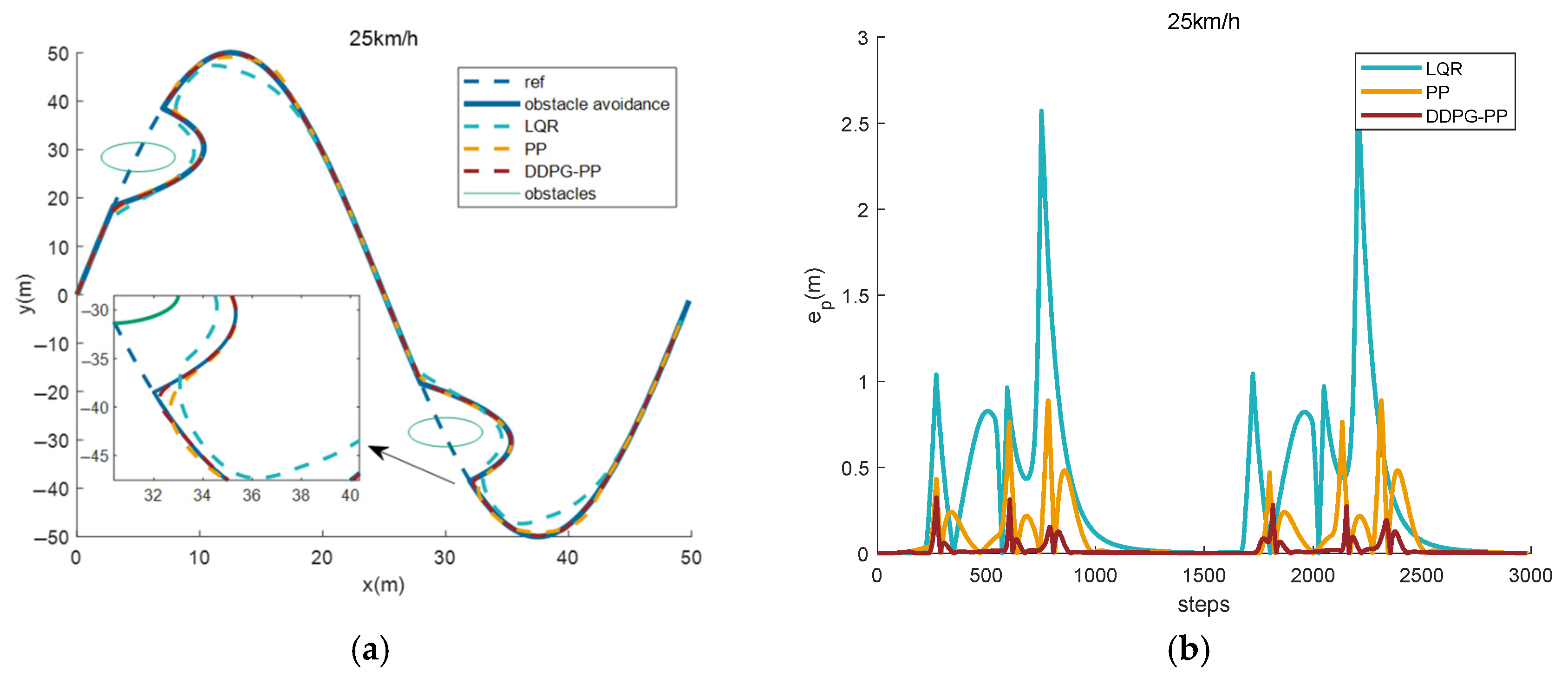
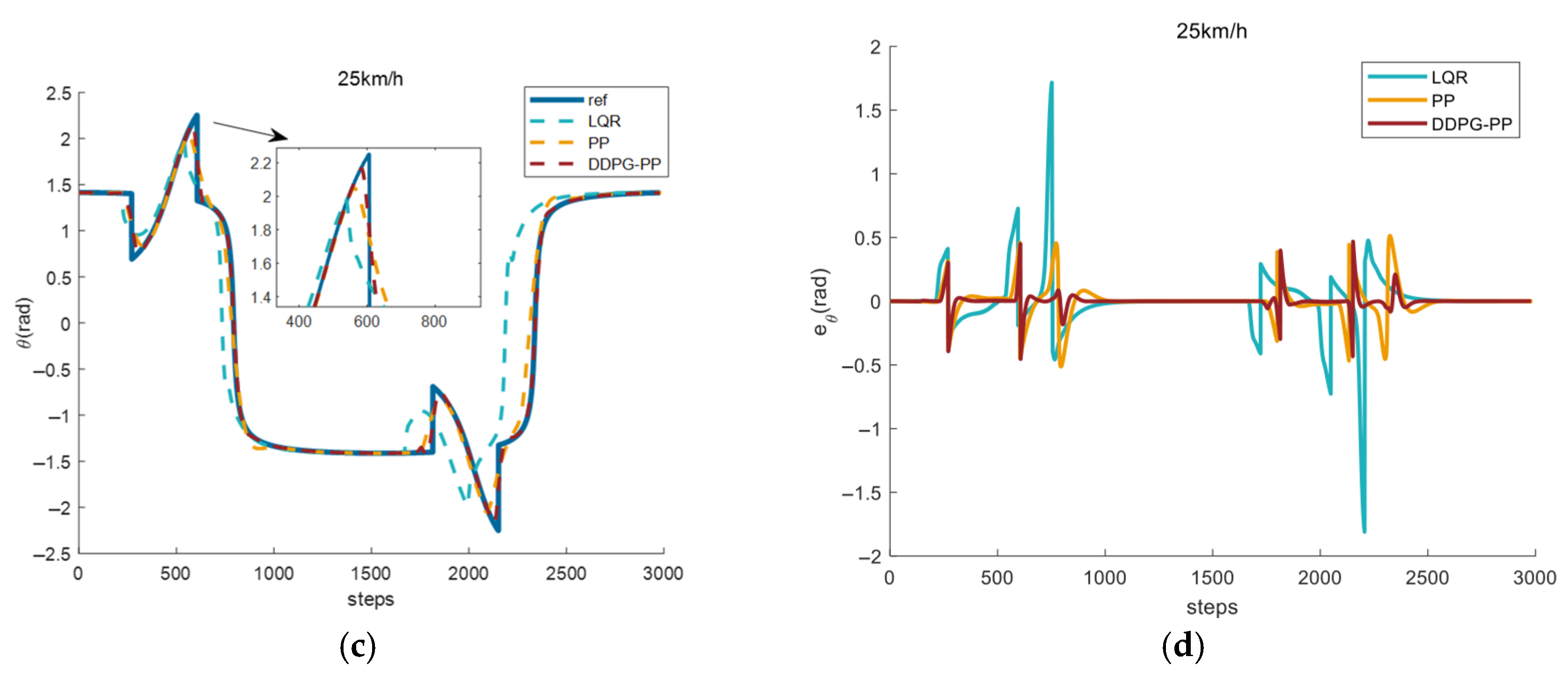
4.3.3. Effect of Path Tracking Under Sinusoidal Function Obstacle Avoidance Paths

In order to verify the effectiveness of the tracked vehicle path tracking algorithm in complex environments, obstacles are introduced into the simulation environment so as to test the adaptability of the algorithm to different obstacle-avoidance situations and verify the robustness of the algorithm. On the basis of the original sin function path, obstacles with a radius of 3 m are set at (5, 28) and (30, −28), and the path is re-planned to obtain the obstacle-avoidance path based on the sin function. The path tracking of this path is shown in Figure 10.

It can be seen from the figure that the maximum value of error still occurs during steering, and the value of the error is amplified compared to the unobstructed path. This indicates that the motion control of tracked vehicles faces greater challenges during steering. Among them, the proposed algorithms are better than the comparison algorithms in fitting the path in the obstacle-avoidance environment. Evaluation metrics are used to quantify the tracking effect, and the specific comparison results are summarized in

Table 6. Path tracking results of different methods under obstacle avoidance conditions.

Method	Evaluation Indicators
	${\mathit{e}}_{\mathbf{p}}$ (m)	${\mathit{e}}_{\mathbf{p}\mathbf{m}\mathbf{a}\mathbf{x}}$ (m)	${\mathit{e}}_{\mathsf{\theta }}$ (rad)	${\mathit{e}}_{\mathsf{\theta }\mathbf{m}\mathbf{a}\mathbf{x}}$ (rad)
LQR	0.3635	2.6414	0.1089	1.8106
PP	0.1051	0.8882	0.0610	0.5136
DDPG-PP	0.0219	0.3237	0.0214	0.4689

.

The average tracking error and the maximum tracking error of DDPG-PP are the smallest among the three methods. The value of the average tracking error is 0.0219, which is 94.0% and 79.2% lower than the LQR method as well as the PP method, respectively. The maximum tracking error is 0.3237, which is 87.7% and 63.6% lower than the LQR and PP methods, respectively. This indicates that DDPG-PP has a significant advantage in this metric and is able to track the path better. The mean heading error and maximum heading error are also the smallest among the three methods, with a value of 0.0214, which is 80.4% and 65.0% lower than the LQR and PP methods, respectively. The maximum heading error is 0.4689, which is 73.0% and 8.7% lower than the LQR and PP methods, respectively. This indicates that the DDPG-PP method is able to track the path heading better.

4.3.4. Effect of Path Tracking Under Complex Road Conditions

In order to verify the control effect of the controller under complex working conditions, a path tracking simulation was carried out under complex road conditions, where the path included multiple curvature changes [10]. The path tracking control effect is shown in Figure 11.

From the figure, it can be seen that the maximum value of error occurs in the steering phase. Among them, the proposed algorithm is better than the comparison algorithms in tracking the paths under complex paths. The tracking effectiveness is quantified using evaluation metrics, and the specific comparison results are summarized in

Table 7. Path tracking results of different methods under complex road conditions.

Method	Evaluation Indicators
	${\mathit{e}}_{\mathbf{p}}$ (m)	${\mathit{e}}_{\mathbf{p}\mathbf{m}\mathbf{a}\mathbf{x}}$ (m)	${\mathit{e}}_{\mathsf{\theta }}$ (rad)	${\mathit{e}}_{\mathsf{\theta }\mathbf{m}\mathbf{a}\mathbf{x}}$
LQR	0.2530	0.7185	0.0277	0.3489
PP	0.0526	0.3079	0.0164	0.2657
DDPG-PP	0.0139	0.1832	0.0097	0.1954

.

The average tracking error and the maximum tracking error of DDPG-PP are the smallest among the three methods. Its average tracking error value is 0.0139; the maximum tracking error is 0.1832. This indicates that DDPG-PP has a significant advantage in this metric and is able to track the path better. In addition, the average heading error and the maximum heading error of DDPG-PP are also the smallest among the three methods: the average heading error is 0.0097; and the maximum heading error is 0.1954, which indicates that the DDPG-PP method is able to track the path heading more accurately. The experimental results show that the proposed method still has a better tracking effect under the complex path conditions where the curvature changes continuously.

5. Conclusions

In order to improve the path tracking accuracy of tracked unmanned vehicles, this paper proposes a path tracking hierarchical control method based on DDPG-PP. Firstly, the upper controller uses the DDPG algorithm to construct an adaptive look-ahead distance optimizer. The look-ahead distance is dynamically adjusted using a reinforcement learning strategy, with the aim of minimizing the path tracking error. Secondly, the model is trained via reinforcement learning with a variety of randomly generated paths, which significantly enhances the generalization ability of the algorithm. Finally, based on the PP algorithm, the lower controller calculates the torque required for the steering of the driving wheels according to the optimal look-ahead distance output from the upper layer, achieving high-precision closed-loop control. The proposed method is compared to the PP and LQR methods to experimentally verify the superiority of the proposed method in terms of average tracking error, average heading error, response time, etc. The experimental results show that the average tracking error in the obstacle avoidance environment is reduced by 94.0% and 79.2% with respect to the LQR method and the PP method, respectively; the maximum tracking error is reduced by 87.7% and 63.6% with respect to the LQR method and the PP method, respectively; the average heading error is reduced by 80.4% and 65.0% with respect to the LQR method and the PP method, respectively; the maximum heading error is reduced by 73.0% and 8.7% with respect to the LQR method and the PP method, respectively; and the response time is improved by 39% and 6% with respect to the LQR method and the PP method, respectively. This indicates that the proposed method reduces the tracking error and improves the response speed at the same time.

In this paper, a hierarchical control method based on DDPG-PP is proposed for improving the path tracking accuracy of tracked unmanned vehicles. Although the method shows good performance in theory and during experiments, there are still some directions that deserve further exploration. Firstly, this paper considers the design of a lateral control system for tracked unmanned vehicles, but does not consider the influence of changes and disturbances in longitudinal control, and the next step will be to consider combining the design of longitudinal control to build a more complete intelligent driving tracking control system. In addition, this paper is mainly a simulation and verification in a computer environment, and further practical verification will be needed in the future.

References

1. Wang, X.; Wang, Y.; Sun, Q.; Chen, Y.; Al-Zahran, A. Adaptive Robust Control of Unmanned Tracked Vehicles for Trajectory Tracking Based on Constraint Modeling and Analysis. Nonlinear Dyn. 2024, 112, 9117–9135. [Google Scholar] [CrossRef]
2. Yao, J.; Li, X.; Zhang, Y.; Chen, K.; Zhang, D.; Ji, J. Autonomous Navigation Control of Tracked Unmanned Vehicle Formation in Communication Restricted Environment. IEEE Trans. Veh. Technol. 2024, 73, 16063–16075. [Google Scholar] [CrossRef]
3. Zhang, Y.; Huang, T. Research on a Tracked Omnidirectional and Cross-Country Vehicle. Mech. Mach. Theory 2015, 87, 18–44. [Google Scholar] [CrossRef]
4. Yue, B.; Zhang, Z.; Zhang, W.; Luo, X.; Zhang, G.; Huang, H.; Wu, X.; Bao, K.; Peng, M. Design of an Automatic Navigation and Operation System for a Crawler-Based Orchard Sprayer Using GNSS Positioning. Agronomy 2024, 14, 271. [Google Scholar] [CrossRef]
5. Hu, C.; Ru, Y.; Li, X.; Fang, S.; Zhou, H.; Yan, X.; Liu, M.; Xie, R. Path Tracking Control for Brake-Steering Tracked Vehicles Based on an Improved Pure Pursuit Algorithm. Biosyst. Eng. 2024, 242, 1–15. [Google Scholar] [CrossRef]
6. Farag, W. Complex Trajectory Tracking Using PID Control for Autonomous Driving. Int. J. ITS Res. 2020, 18, 356–366. [Google Scholar] [CrossRef]
7. Mai, T.A. A Combined Backstepping and Adaptive Fuzzy PID Approach for Trajectory Tracking of Autonomous Mobile Robots. J. Braz. Soc. Mech. Sci. Eng. 2021, 43, 156. [Google Scholar] [CrossRef]
8. Han, J.; Wang, P.; Yang, X. Tuning of PID Controller Based on Fruit Fly Optimization Algorithm. In Proceedings of the 2012 IEEE International Conference on Mechatronics and Automation, Chengdu, China, 5–8 August 2012; pp. 409–413. [Google Scholar]
9. Vo, A.T.; Kang, H.-J. A Chattering-Free, Adaptive, Robust Tracking Control Scheme for Nonlinear Systems with Uncertain Dynamics. IEEE Access 2019, 7, 10457–10466. [Google Scholar] [CrossRef]
10. Yang, T.; Bai, Z.; Li, Z.; Feng, N.; Chen, L. Intelligent Vehicle Lateral Control Method Based on Feedforward + Predictive LQR Algorithm. Actuators 2021, 10, 228. [Google Scholar] [CrossRef]
11. Fan, Z.; Yan, Y.; Wang, X.; Xu, H. Path Tracking Control of Commercial Vehicle Considering Roll Stability Based on Fuzzy Linear Quadratic Theory. Machines 2023, 11, 382. [Google Scholar] [CrossRef]
12. Park, M.; Yim, S. Design of a Path-Tracking Controller with an Adaptive Preview Distance Scheme for Autonomous Vehicles. Machines 2024, 12, 764. [Google Scholar] [CrossRef]
13. Kim, H.; Kim, D.; Shu, I.; Yi, K. Time-Varying Parameter Adaptive Vehicle Speed Control. IEEE Trans. Veh. Technol. 2016, 65, 581–588. [Google Scholar] [CrossRef]
14. Ding, C.; Ding, S.; Wei, X.; Mei, K. Composite SOSM Controller for Path Tracking Control of Agricultural Tractors Subject to Wheel Slip. ISA Trans. 2022, 130, 389–398. [Google Scholar] [CrossRef]
15. Elbanhawi, M.; Simic, M.; Jazar, R. Receding Horizon Lateral Vehicle Control for Pure Pursuit Path Tracking. J. Vib. Control 2018, 24, 619–642. [Google Scholar] [CrossRef]
16. Jiang, X.; Kuroiwa, T.; Cao, Y.; Sun, L.; Zhang, H.; Kawaguchi, T.; Hashimoto, S. Enhanced Pure Pursuit Path Tracking Algorithm for Mobile Robots Optimized by NSGA-II with High-Precision GNSS Navigation. Sensors 2025, 25, 745. [Google Scholar] [CrossRef] [PubMed]
17. Qinpeng, S.; Zhonghua, W.; Meng, L.; Bin, L.; Jin, C.; Jiaxiang, T. Path Tracking Control of Wheeled Mobile Robot Based on Improved Pure Pursuit Algorithm. In Proceedings of the 2019 Chinese Automation Congress (CAC), Hangzhou, China, 22–24 November 2019; pp. 4239–4244. [Google Scholar]
18. Huang, Y.; Tian, Z.; Jiang, Q.; Xu, J. Path Tracking Based on Improved Pure Pursuit Model and PID. In Proceedings of the 2020 IEEE 2nd International Conference on Civil Aviation Safety and Information Technology (ICCASIT.), Weihai, China, 14 October 2020; pp. 359–364. [Google Scholar]
19. Ahn, J.; Shin, S.; Kim, M.; Park, J. Accurate Path Tracking by Adjusting Look-Ahead Point in Pure Pursuit Method. Int. J. Automot. Technol. 2021, 22, 119–129. [Google Scholar] [CrossRef]
20. Zhang, D.; Wang, Y.; Meng, L.; Yan, J.; Qin, C. Adaptive Critic Design for Safety-Optimal FTC of Unknown Nonlinear Systems with Asymmetric Constrained-Input. ISA Trans. 2024, 155, 309–318. [Google Scholar] [CrossRef]
21. Chen, J.; Jiang, Y.; Pan, H.; Yang, M. Path Planning in Complex Environments Using Attention-Based Deep Deterministic Policy Gradient. Electronics 2024, 13, 3746. [Google Scholar] [CrossRef]
22. Sun, Y.; Yuan, B.; Zhang, Y.; Zheng, W.; Xia, Q.; Tang, B.; Zhou, X. Research on Action Strategies and Simulations of DRL and MCTS-Based Intelligent Round Game. Int. J. Control Autom. Syst. 2021, 19, 2984–2998. [Google Scholar] [CrossRef]
23. Vo, A.K.; Mai, T.L.; Yoon, H.K. Path Planning for Automatic Berthing Using Ship-Maneuvering Simulation-Based Deep Reinforcement Learning. Appl. Sci. 2023, 13, 12731. [Google Scholar] [CrossRef]
24. Woo, J. Deep Reinforcement Learning-Based Controller for Path Following of an Unmanned Surface Vehicle. Ocean Eng. 2019, 183, 155–166. [Google Scholar] [CrossRef]
25. Yao, J.; Ge, Z. Path-Tracking Control Strategy of Unmanned Vehicle Based on DDPG Algorithm. Sensors 2022, 22, 7881. [Google Scholar] [CrossRef] [PubMed]
26. Niu, S.; Pan, X.; Wang, J.; Li, G. Deep Reinforcement Learning from Human Preferences for ROV Path Tracking. Ocean Eng. 2025, 317, 120036. [Google Scholar] [CrossRef]
27. Zhang, L.; Zhang, R.; Zhang, D.; Yi, T.; Ding, C.; Chen, L. Path Curvature Incorporated Reinforcement Learning Method for Accurate Path Tracking of Agricultural Vehicles. Comput. Electron. Agric. 2025, 234, 110243. [Google Scholar] [CrossRef]
28. Cheng, X.; Zhang, S.; Cheng, S.; Xia, Q.; Zhang, J. Path-Following and Obstacle Avoidance Control of Nonholonomic Wheeled Mobile Robot Based on Deep Reinforcement Learning. Appl. Sci. 2022, 12, 6874. [Google Scholar] [CrossRef]
29. Zheng, Y.; Tao, J.; Hartikainen, J.; Duan, F.; Sun, H.; Sun, M.; Sun, Q.; Zeng, X.; Chen, Z.; Xie, G. DDPG Based LADRC Trajectory Tracking Control for Underactuated Unmanned Ship under Environmental Disturbances. Ocean Eng. 2023, 271, 113667. [Google Scholar] [CrossRef]
30. Wang, X.; Yuan, Y.; Tong, L.; Yuan, C.; Shen, B.; Long, T. Energy Management Strategy for Diesel–Electric Hybrid Ship Considering Sailing Route Division Based on DDPG. IEEE Trans. Transp. Electrific. 2024, 10, 187–202. [Google Scholar] [CrossRef]
31. Vouros, G.A. Explainable Deep Reinforcement Learning: State of the Art and Challenges. ACM Comput. Surv. 2023, 55, 1–39. [Google Scholar] [CrossRef]
32. Liu, J.; Huang, Z.; Xu, X.; Zhang, X.; Sun, S.; Li, D. Multi-Kernel Online Reinforcement Learning for Path Tracking Control of Intelligent Vehicles. IEEE Trans. Syst. Man Cybern. Syst. 2021, 51, 6962–6975. [Google Scholar] [CrossRef]
33. Qin, C.; Qiao, X.; Wang, J.; Zhang, D.; Hou, Y.; Hu, S. Barrier-Critic Adaptive Robust Control of Nonzero-Sum Differential Games for Uncertain Nonlinear Systems With State Constraints. IEEE Trans. Syst. Man Cybern. Syst. 2024, 54, 50–63. [Google Scholar] [CrossRef]
34. Qin, C.; Jiang, K.; Wang, Y.; Zhu, T.; Wu, Y.; Zhang, D. Event-Triggered H∞ Control for Unknown Constrained Nonlinear Systems with Application to Robot Arm. Appl. Math. Model. 2025, 144, 116089. [Google Scholar] [CrossRef]
35. Wu, J.; Zou, Y.; Zhang, X.; Du, G.; Du, G.; Zou, R. A Hierarchical Energy Management for Hybrid Electric Tracked Vehicle Considering Velocity Planning With Pseudospectral Method. IEEE Trans. Transp. Electrif. 2020, 6, 703–716. [Google Scholar] [CrossRef]
36. Cao, Y.; Ni, K.; Kawaguchi, T.; Hashimoto, S. Path Following for Autonomous Mobile Robots with Deep Reinforcement Learning. Sensors 2024, 24, 561. [Google Scholar] [CrossRef] [PubMed]
Figure 1. Schematic diagram of steering a crawler vehicle.
Machines 13 00603 g001
Figure 2. Path tracking hierarchical control strategy based on DDPG-PP.
Machines 13 00603 g002
Figure 3. DDPG based path tracking controller.
Machines 13 00603 g003
Figure 4. Randomized path generated based on the path generation algorithm.
Machines 13 00603 g004
Figure 5. Schematic diagram of the PP algorithm.
Machines 13 00603 g005
Figure 6. Reward curve diagram.
Machines 13 00603 g006
Figure 7. Tracking effect of different path tracking methods at different speeds. (a) Path tracking curve at 10 km/h. (b) Path tracking error at 10 km/h. (c) Path tracking curve at 20 km/h. (d) Path tracking error at 20 km/h. (e) Path tracking curve at 30 km/h. (f) Path tracking error at 30 km/h. (g) Path tracking curve at 40 km/h. (h) Path tracking error at 40 km/h.
Machines 13 00603 g007
Figure 8. Path tracking effect of different methods under straight paths. (a) Path tracking curves under straight paths. (b) Path tracking error under straight paths. (c) Heading tracking curves under straight-line paths. (d) Heading tracking error under a straight path.
Machines 13 00603 g008
Figure 9. Path tracking effect of different methods under sin function paths. (a) Path tracking curves under sin-shaped paths. (b) Path tracking error under sin-shaped paths. (c) Heading tracking curves under sin-shaped paths. (d) Heading tracking error under sin-shaped paths.
Machines 13 00603 g009
Figure 10. Path tracking effect of different methods under obstacle avoidance conditions. (a) Path tracking curves under obstacle avoidance paths. (b) Path tracking error under obstacle avoidance paths. (c) Heading tracking curves under obstacle avoidance paths. (d) Heading tracking error under obstacle avoidance paths.
Machines 13 00603 g010aMachines 13 00603 g010b
Figure 11. Path tracking effect of different methods under complex road conditions. (a) Path tracking curves under complex road conditions. (b) Path tracking error under complex road conditions. (c) Heading tracking curves under complex road conditions. (d) Heading tracking error under complex road conditions.
Machines 13 00603 g011