Remaining Useful Life Prediction of Aero-Engine Based on Improved GWO and 1DCNN

Abstract

With the deepening adoption of whole-lifecycle management paradigms in aviation equipment, accurate prediction of remaining useful life has emerged as a pivotal technical enabler for ensuring flight safety and optimizing maintenance resource allocation. This study systematically addresses limitations in existing data-driven remaining useful life prediction methodologies through comprehensive optimizations spanning data preprocessing protocols and model architectural enhancements. To mitigate the local optimum entrapment inherent in deep learning hyperparameter optimization, an improved Gray Wolf Optimizer incorporating dynamic perturbation factors is proposed. This algorithm is subsequently deployed to optimize hyperparameters within the redesigned predictive architecture. Comparative analyses reveal that the proposed framework achieves superior prediction accuracy compared to mainstream optimization-driven models and state-of-the-art approaches. The results substantiate the capability of dynamic perturbation strategies to enhance both hyperparameter optimization quality and prediction stability, ultimately delivering an efficient solution for aero-engine remaining useful life estimation. The experiments on the C-MAPSS Dataset verify the effectiveness of these improvements.

1. Introduction

Aero-engines, as the core propulsion systems in modern aerospace engineering, have evolved from piston-based architectures to complex configurations such as turbofan and turbine engines. While this structural advancement has significantly improved operational performance, it has simultaneously led to a notable increase in both fault frequency and diversity [1]. Statistical data indicate that approximately 60% of aviation accidents in China over the past decade were attributed to engine-related failures [2]. The two Airbus A330 accidents in 2017 and 2023, both triggered by blade damage, empirically validate the critical role of engine reliability in ensuring flight safety [3]. Conventional maintenance strategies based on fixed schedules or post-failure interventions suffer from dual limitations of “under-maintenance” and “over-maintenance”, resulting in substantial financial costs. Engine maintenance alone accounts for 40% of total aircraft operational expenditures, posing significant economic challenges to both defense and civil aviation sectors [4,5]. This underscores the urgent need for innovative maintenance paradigms. RUL prediction technology can provide high-precision assessments of engine health status, supporting scientific and refined maintenance decision-making, thereby minimizing the risk of sudden safety accidents caused by equipment failures, and ensuring the stability and safety of flight missions. Additionally, accurate RUL predictions can reduce unnecessary parts maintenance and replacement, optimize maintenance strategies, lower maintenance costs, and maximize the service efficiency of the engine. By reasonably planning maintenance cycles and optimizing resource allocation, it is possible to effectively reduce task interruptions caused by sudden failures, thereby enhancing the overall stability and reliability of operations. Therefore, accurately predicting the remaining useful life of aviation engines and achieving efficient predictive maintenance is an important means to address the drawbacks of current traditional maintenance methods, and it is a key strategy to improve safety, economy, and operational efficiency in the aviation industry. At present, RUL prediction methods are mainly divided into three categories: physics-based models, data-driven methods, and hybrid methods [6]. While physics-based approaches provide mechanistic interpretability, their effectiveness is fundamentally constrained by the inherent complexity of modeling degradation processes under multifaceted operational conditions. Data-driven methodologies, conversely, circumvent these limitations by establishing machine learning-enabled correlations between operational data patterns and system degradation, requiring no explicit physical formulations while demonstrating superior adaptability in practical health management scenarios.

The fundamental objective of RUL prediction lies in accurately estimating the remaining lifespan from the current operational state to functional failure through real-time monitoring and analysis, thereby providing critical support for optimizing maintenance strategies and reducing operational costs [7]. Despite theoretical and practical advancements in RUL prediction, the inherent complexity of degradation processes and the high-dimensional nature of operational data continue to pose significant challenges in achieving efficient and precise life estimation. In response to these challenges, researchers have increasingly explored data-driven prediction frameworks, leveraging machine learning algorithms to extract latent features from operational data as novel solutions for RUL estimation [8,9,10,11]. For instance, Khelif et al. employed support vector regression to establish nonlinear mappings between critical turbine engine features and remaining lifespan [12]. Sbarufatti et al. integrated multilayer perceptrons with sequential Monte Carlo filters to predict the remaining life of structural components affected by fatigue crack propagation, utilizing the perceptrons’ nonlinear modeling capabilities for crack growth dynamics while dynamically refining predictions through Monte Carlo filtering [13]. Alfarizi et al. adopted empirical mode decomposition for preprocessing non-stationary vibration signals, subsequently constructing prediction models via Bayesian-optimized random forests [14]. While these studies demonstrate scenario-specific effectiveness, their performance heavily relies on meticulous feature engineering and exhibits limitations in modeling complex temporal dependencies. Challenges persist in maintaining generalization capability and prediction stability when addressing long-term dependencies, noise interference, or high-dimensional nonlinear datasets.

Deep learning, as a pivotal branch of machine learning, effectively addresses multiple limitations inherent to traditional approaches in RUL prediction. Primarily, deep neural networks exhibit feature self-extraction capability, autonomously learning complex nonlinear patterns directly from raw operational data, thereby reducing reliance on manual feature engineering. Furthermore, these models demonstrate exceptional competence in processing multi-sensor temporal sequences, achieving breakthroughs in scenarios where conventional machine learning methods underperform [15]. Kong et al. developed deep learning approaches for the velocity field prediction in a scramjet isolator [16] and flow field prediction [17]. Ma et al. proposed a Deep-convolution-based LSTM network for remaining useful life prediction [18]. Zheng et al. developed an LSTM-based prognostic framework that enhances prediction accuracy through effective modeling of long-term dependencies in temporal sequences [19]. Wang et al. proposed a recurrent–convolutional hybrid architecture to address temporal dependencies and prediction uncertainty in degradation processes, achieving synergistic optimization of temporal modeling and feature abstraction [20]. Luo et al. introduced a multi-scale temporal convolutional network that adaptively integrates degradation features across varying time spans, demonstrating improved robustness under complex operating conditions and multi-failure scenarios [21]. The 1D convolutional neural network (1D-CNN), specifically tailored for aero-engine RUL prediction, exhibits unique advantages in processing multivariate time-series sensor data. Its architecture—comprising convolutional layers, activation functions, pooling operations, and fully connected layers—enables hierarchical abstraction of local features into global degradation patterns, ultimately mapping to continuous RUL estimations [22]. Unlike traditional methods dependent on empirical feature design, 1D-CNN autonomously extracts lifespan-critical features from raw signals, minimizing human intervention and potential information loss. The localized convolution and pooling operations inherently suppress measurement noise, while parameter-sharing mechanisms mitigate overfitting risks, collectively ensuring consistent prediction accuracy under varying operational conditions.

Despite the demonstrated efficacy of deep learning-based approaches in aero-engine RUL prediction, significant challenges persist in practical implementations. Deep neural architectures inherently involve numerous hyperparameters whose optimal configurations require exhaustive exploration within high-dimensional, nonlinear, and multimodal parameter spaces. Conventional strategies—including grid search, random search, and expert-driven manual tuning—suffer from prohibitive computational inefficiency, as the combinatorial explosion of hyperparameter combinations leads to exponential escalation in optimization time costs, rendering them impractical for real-time engineering applications. While existing studies have employed classical intelligent optimization algorithms to enhance hyperparameter tuning efficiency, these methods remain susceptible to local optimum entrapment. Particularly in high-dimensional search spaces, they struggle to balance exploration–exploitation trade-offs, often failing to converge toward theoretically optimal configurations. This limitation fundamentally constrains the achievable performance ceiling of predictive models, especially when addressing complex degradation patterns with multiple interacting failure modes.

To address the challenges of numerous hyperparameters in deep learning models and the inefficiencies of conventional optimization methods reliant on expert experience, this investigation focuses on intelligent optimization algorithms for hyperparameter configuration. Among these algorithms, the Genetic Algorithm (GA) explores parameter combinations through simulated biological evolutionary mechanisms (selection, crossover, mutation), yet its effectiveness diminishes in high-dimensional spaces due to dependency on intricate hyperparameter settings [23]. Particle Swarm Optimization (PSO) updates parameters via swarm intelligence, demonstrating rapid initial convergence but exhibiting sensitivity to population initialization and susceptibility to premature convergence in local optima [24]. In contrast, the Gray Wolf Optimizer (GWO) emulates the hierarchical hunting behavior of wolf packs, guided by alpha, beta, and delta leaders to direct search trajectories. Its incorporation of an adaptive convergence factor dynamically modulates global exploration and local exploitation, endowing the algorithm with structural simplicity, low parametric dependency, and enhanced robustness in high-dimensional non-convex optimization scenarios [25]. These inherent advantages position GWO as a particularly suitable candidate for hyperparameter tuning in complex deep learning architectures tasked with modeling intricate degradation patterns.

While the Gray Wolf Optimizer demonstrates notable advantages in complex optimization problems through its social hierarchy mechanisms and reduced parametric dependency, inherent limitations persist in practical implementations. The algorithm’s position-updating strategy inherently risks premature convergence and local optimum entrapment, particularly when handling non-convex, multimodal search spaces, thereby limiting global search capacity. To mitigate these constraints, this study proposes an improved GWO variant incorporating dynamic perturbation factors during the position-updating phase. This modification strategically balances exploration–exploitation dynamics by adaptively adjusting search step sizes based on iterative progression, thereby refining both the quality and stability of identified hyperparameter configurations. The improved algorithm is subsequently applied to optimize the architectural parameters of the proposed prediction model.

This investigation advances current data-driven RUL prediction frameworks through systematic refinement of prognostic network architectures, focusing on parametric optimization to enhance feature representation learning and temporal dependency capture. The proposed methodology, rigorously validated via NASA’s C-MAPSS benchmarks, demonstrates improved prediction accuracy while maintaining operational feasibility, thereby establishing a generalized framework for remaining life estimation in aerospace propulsion systems.

2. Theoretical Background

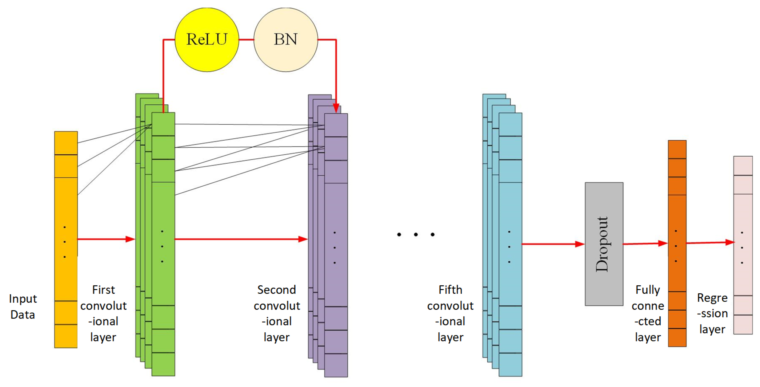
2.1. 1D Convolutional Neural Network

The 1D convolutional neural network (1D-CNN), a deep learning architecture specifically designed for temporal signal processing, operates through local receptive fields and weight-sharing mechanisms to extract local temporal dependencies along the sequential dimension. And the 1D-CNN structure is illustrated in Figure 1.

Unlike conventional 2D-CNNs primarily applied in image processing—where convolutional kernels slide across spatial dimensions (height and width)—the 1D-CNN executes unidirectional kernel sliding along the temporal axis, capturing inter-step correlations between adjacent time points. This architectural specialization significantly reduces parameter dimensionality while preserving temporal structural features, making it particularly suited for processing sensor-derived data streams with inherent sequential characteristics. The distinct advantage of 1D-CNN lies in its capacity to precisely identify latent dynamic patterns and evolutionary trends embedded within time-series data. These capabilities underpin its superior performance in temporal analysis and prediction tasks, especially in industrial applications such as mechanical equipment remaining life prognosis. The network architecture comprises the following core components:

(1)

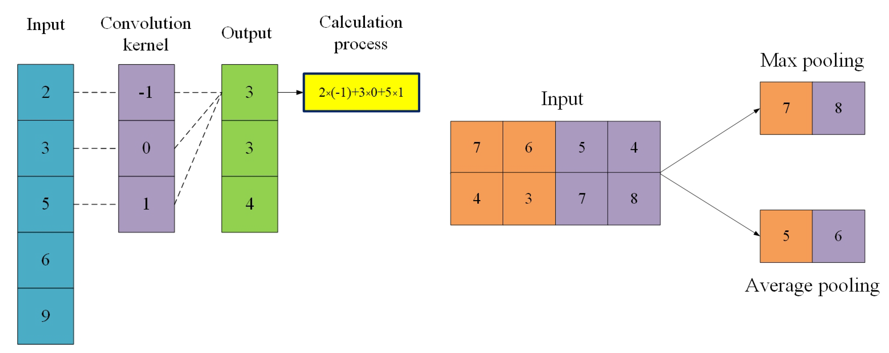
The convolution layer serves as the core structure of the 1DCNN. This layer slides the convolution kernel along the time axis to scan the input data and performs convolution operations on the input [26], as shown in Equation (1), and the convolution calculation process is illustrated in Figure 2:

$$y_n^{(m+1)}(p)=L_n^m\cdot X^m(p)+Z_n^m$$

(1)

In this formulation, $L_n^m$ and $Z_n^m$ denote the weight and bias of the n-th convolutional kernel in the m-th layer, respectively. $X^m(p)$ denotes the p-th local receptive field within the input feature map of the m-th layer, and $y_n^{(m+1)}(p)$ represents the pre-activation input to the p-th neuron in the output feature map generated by the n-th convolutional kernel of the (m + 1)-th layer.

(2)

Normalization layer standardizes the feature distribution of each training batch by rescaling the data to zero mean and unit variance, subsequently restoring representational flexibility through learnable scaling and shifting parameters. This technique effectively mitigates vanishing/exploding gradient issues while enabling higher learning rates and reducing sensitivity to parameter initialization. It is conventionally implemented between convolutional operations and activation functions.

(3)

The pooling layer serves to perform localized information compression on temporal data through dimensionality reduction, thereby reducing computational complexity while enhancing model robustness against data noise. Common implementations include max pooling and average pooling operations, which, respectively, extract dominant features via local maxima detection and suppress fluctuations through regional averaging, with their mechanistic principles systematically illustrated in Figure 2.

(4)

The activation layer introduces nonlinear mapping capabilities through activation functions, thereby enabling the modeling of complex decision boundaries. Four predominant activation functions are commonly employed in practice, with their mathematical formulations detailed in Equations (2)–(5):

$$\tanh (x)={\displaystyle \frac{e^x-e^{-x}}{e^x+e^{-x}}}$$

(2)

$$\mathrm{Sigmoid}(x)={\displaystyle \frac{1}{1+e^{-x}}}$$

(3)

$$\mathrm{ReLU}(x)=\max (0,x)$$

(4)

$$\mathrm{Elu}(x)=\left\{\begin{array}{ll}x,\hfill & x>0\hfill \\ e^x-1,\hfill & x\le 0\hfill \end{array}\right.$$

(5)

(5)

The fully connected layer transforms the extracted spatiotemporal features into a high-dimensional vector through flattening operations, thereby establishing global correlations via weight matrix-mediated linear projection from feature space to task space. This structural component integrates hierarchical features from preceding layers while preserving critical discriminative information, ultimately generating refined feature representations for regression layer processing. The mathematical formulation governing this transformation is provided in Equation (6).

$$y^{l+1(j)}={\displaystyle \sum _{i=1}^n{W}_{ij}^l}{x}^{l(i)}+b_j^l$$

(6)

In this mathematical representation, W^l_ij denotes the weight parameter connecting the i-th neuron in layer l to the corresponding j-th neuron in layer l + 1. b^l_j represents the bias term propagated from layer l to the j-th neuron in layer l + 1. x^l(i) corresponds to the output value of the i-th neuron in layer l, while b^l_j signifies the output response value of the j-th neuron in layer l + 1.

2.2. Gray Wolf Optimization Algorithm

The Gray Wolf Optimizer (GWO) is a metaheuristic optimization algorithm inspired by the social hierarchy and cooperative hunting strategies of gray wolf populations, initially proposed by Mirjalili et al. in 2014 [27]. Within this framework, the wolf pack’s hierarchical structure—comprising four distinct tiers (alpha (α), beta (β), delta (δ), and omega (ω))—is abstracted into a search mechanism for solution space exploration. The alpha wolves, as dominant leaders, guide decision-making processes, beta wolves act as secondary decision supporters, delta wolves perform scouting and territorial guarding roles, while omega wolves maintain social equilibrium by following higher-ranked members. In algorithmic terms, this social hierarchy translates to a dynamic optimization strategy: α, β, and δ wolves represent the current iteration’s optimal, suboptimal, and tertiary solutions, respectively. The remaining candidate solutions (ω wolves) iteratively update their positions by emulating the leadership triad, collectively driving the swarm toward globally optimal regions. The hunting behavior of gray wolves is algorithmically decomposed into three sequential phases—searching, encircling, and attacking—which are mechanically abstracted into mathematical formulations governing the optimization process [27]. During the initial exploration phase, the wolves collaboratively narrow the encirclement around potential prey positions through coordinated spatial perception. This behavioral sequence is mathematically represented by Equations (7)–(10):

$$\mathit{D}=\left|\mathit{C}\cdot {\mathit{X}}_p\left(t\right)-\mathit{X}\left(t\right)\right|$$

(7)

$$\mathit{X}(t+1)={\mathit{X}}_p(t)-\mathit{A}\cdot \mathit{D}$$

(8)

$$\mathit{A}=2\mathit{a}\cdot {\mathit{r}}_1-\mathit{a}$$

(9)

$$\mathit{C}=2\cdot {\mathit{r}}_2$$

(10)

In the formalism, D represents the distance vector emulating the spatial separation between the wolf pack and prey; X_p denotes the prey’s current position vector (corresponding to the incumbent optimal solution); X signifies the position vector of an individual gray wolf; A and C are coefficient vectors governing exploration–exploitation dynamics, where A modulates the attack intensity; a is a convergence factor that linearly decreases from 2 to 0 over iterations; r₁ and r₂ are random vectors within [0, 1], serving as stochastic components to balance global exploration and local exploitation capabilities; and t indicates the current iteration index.

During the hunting process, the positional information of α, β, and δ wolves dictates the collective movement of the swarm. The algorithm updates the positions of individual wolves through a weighted averaging strategy, where ω wolves iteratively adjust their locations under the guidance of the α, β, and δ leaders. This hierarchical coordination mechanism ensures progressive convergence toward global optima, with the position-updating dynamics mathematically formalized as follows:

$${\mathit{D}}_{\mathsf{\alpha }}=\left|{\mathit{C}}_1\cdot {\mathit{D}}_{\mathsf{\alpha }}-\mathit{X}\right|$$

(11)

$${\mathit{D}}_{\mathsf{\beta }}=\left|{\mathit{C}}_2\cdot {\mathit{D}}_{\mathsf{\beta }}-\mathit{X}\right|$$

(12)

$${\mathit{D}}_{\mathrm{\delta }}=\left|C_3\cdot {\mathit{D}}_{\mathrm{\delta }}-\mathit{X}\right|$$

(13)

$${\mathit{X}}_1={\mathit{X}}_{\mathrm{\alpha }}-{\mathit{A}}_1\cdot \left({\mathit{D}}_{\mathrm{\alpha }}\right)$$

(14)

$${\mathit{X}}_2={\mathit{X}}_{\mathsf{\beta }}-{\mathit{A}}_2\cdot \left({\mathit{D}}_{\mathsf{\beta }}\right)$$

(15)

$${\mathit{X}}_3={\mathit{X}}_{\mathrm{\delta }}-{\mathit{A}}_3\cdot \left({\mathit{D}}_{\mathrm{\delta }}\right)$$

(16)

$${\mathit{X}}_{\mathsf{\omega }}\left(t+1\right)={\displaystyle \frac{{\mathit{X}}_1+{\mathit{X}}_2+{\mathit{X}}_3}{3}}$$

(17)

Within this mathematical framework, D_α, D_β, and D_δ represent the distance vectors between α, β, and δ wolves and other swarm members, respectively. X_α, X_β, and X_δ denote the current positions of the α, β, and δ leaders, while C₁, C₂, and C₃ are stochastic vectors introducing randomness into the search process. The relative displacement vectors X₁, X₂, and X₃ quantify the spatial relationships between ω wolves and the leadership triad, with X_ω(t+1) defining the updated position of ω wolves under hierarchical guidance. This mechanism allows the group to dynamically adjust in the search space, reducing the risk of the model getting trapped in local optima while gradually approaching the potential optimal solution area.

When the prey stops moving, the gray wolf initiates the attack to end the hunt. During the optimization process, the value of A changes within the interval [−a, a] as the value of a changes. When $\mathit{A}$ > 1, the wolf pack conducts a global search, and when $\mathit{A}$ < 1, a local search is performed [28].

The implementation process of the algorithm can be divided into three stages: initialization, fitness evaluation, and iterative optimization. Firstly, the initial positions of the gray wolf population are generated randomly, and the initial value of the control parameter a and the maximum number of iterations are set. In each iteration, the fitness values of the individuals are calculated to update the positions of α, β, and δ, and then the positions of all gray wolves are updated by adjusting the values of $\mathit{A}$ and $\mathit{C}$. Parameter a linearly decreases with the number of iterations, allowing the algorithm to prefer global exploration in the early iterations and focus on local fine search in the later iterations. The iterative process continues until the termination condition is reached, at which point the optimal solution is output.

3. Improved GWO-1DCNN for RUL Prediction of Aero-Engine

3.1. Improvement Strategy of GWO with Dynamic Disturbance Factor

The Gray Wolf Optimizer (GWO) has demonstrated notable advantages in parameter optimization tasks due to its social hierarchy guidance mechanism and hunting behavior simulation strategy, characterized by structural simplicity and efficient convergence characteristics. Compared to the crossover–mutation operations of Genetic Algorithms (GA) or the velocity–position update rules of Particle Swarm Optimization (PSO), GWO drives swarm evolution solely through positional updates guided by the α, β, and δ leaders, significantly reducing algorithmic complexity and parameter tuning costs. However, when applied to high-dimensional, multimodal optimization scenarios—such as hyperparameter tuning for deep learning-based aero-engine RUL prediction—the algorithm’s linearly decreasing position-updating parameters, though theoretically balancing global exploration and local exploitation, suffer from limitations. The fixed attenuation pattern risks premature loss of population diversity, often triggering local optima stagnation phenomena in complex search landscapes. This phenomenon typically manifests as late-stage swarm aggregation around suboptimal solutions, with individuals struggling to escape saddle points or navigate narrow valley regions of the objective function.

To address these limitations, this study introduces an improved Gray Wolf Optimizer incorporating a dynamic perturbation factor that progressively diminishes with iteration count, thereby refining the position-updating mechanism. The mathematical formulation of this perturbation factor is defined as follows (Equation (18)).

$$\gamma \left(t\right)={\gamma }_{\max }\cdot (1-{\displaystyle \frac{t}{t_{\max }}})$$

(18)

Among them, ${\gamma }_{\max }$ is the initial set maximum disturbance intensity, $\mathit{t}$ is the current iteration number, and t_max is the maximum iteration number. At the same time, the position update formula of the gray wolf at time $\mathit{t}$ + 1 is optimized to Equation (19):

$${\mathit{X}}_{\mathsf{\omega }}\left(t+1\right)={\displaystyle \frac{{\mathit{X}}_1+{\mathit{X}}_2+{\mathit{X}}_3}{3}}+\gamma \left(t\right)\mathit{R}$$

(19)

In this formulation, the vector R represents a stochastic perturbation vector bounded within the interval [−1, 1], designed to emulate directional randomness in position updates.

The incorporation of a dynamic disturbance factor into the Gray Wolf Optimizer (GWO) is theoretically grounded in addressing premature convergence and local optima stagnation, drawing from stochastic optimization principles and swarm diversity preservation. By introducing controlled noise into the position update equations, the perturbation disrupts the deterministic hunting behavior of wolves, thereby preventing excessive population homogeneity and maintaining exploration capability. This mechanism aligns with the stochastic search theory, ensuring a non-zero probability of escaping local attractors while adaptively balancing exploration and exploitation, initially broadening the search scope and gradually fading for fine-tuning.

This design enhances the robustness of the algorithm through a two-stage strategy: in the early iterations, when the newly added dynamic disturbance factor is large, this disturbance term can widen the search radius of gray wolf individuals, preventing the group from falling into the same area due to excessive following of the leadership hierarchy; in the later iterations, when the dynamic disturbance factor is small, the disturbance amplitude shrinks to ensure that the algorithm searches finely within the neighborhood of potential optimal solutions. Compared to the linear parameter adjustment of traditional GWO, the dynamic disturbance factor introduces a dual mechanism of nonlinear decay and random disturbance, granting the algorithm the adaptive ability to escape local extrema, thereby providing a more stable optimization framework for hyperparameters in the remaining life prediction model of aircraft engines.

Additionally, traditional model update methods often rely on a single partition of the validation set to directly optimize the loss function, and the selection of hyperparameters can be easily influenced by the randomness of data partitioning. For instance, a validation set that inadvertently contains specific operational condition samples may lead the model to converge towards a locally optimal solution. To address this issue, this study adopts a cross-validation strategy as a replacement for the traditional single validation mechanism. Cross-validation is a statistical method that evaluates model performance through multiple partitions of the dataset and iterative validation. The core idea is to reduce the interference of randomness from a single data partition on model optimization by assessing from multiple angles. In the context of remaining useful life prediction for aviation engines, this method essentially divides the complete dataset into several mutually exclusive subsets and employs a rotation of training and validation, ensuring that the model is tested across diverse data distributions, thereby providing a more comprehensive reflection of its generalization potential.

In this study, a five-fold cross-validation strategy was employed to optimize the hyperparameters of the proposed prognostic model. First, the complete engine sensor dataset was uniformly partitioned into five independent subsets according to the chronological order. Each subset contained consecutive and intact operational cycle segments to preserve the temporal correlation of operational condition evolution that could be disrupted by random partitioning. Subsequently, each subset was sequentially designated as the validation set, while the remaining four subsets were merged into the training set, forming five distinct training–validation combinations. During each training iteration, the model updated its hyperparameters using the Gray Wolf Optimizer, with the mean absolute error (MAE) of the validation set serving as the loss function. Finally, the average value of the validation results from the five folds was adopted as the ultimate evaluation metric for the performance of the current hyperparameter configuration.

3.2. RUL Prediction of Aero-Engine Based on Improved GWO-1DCNN

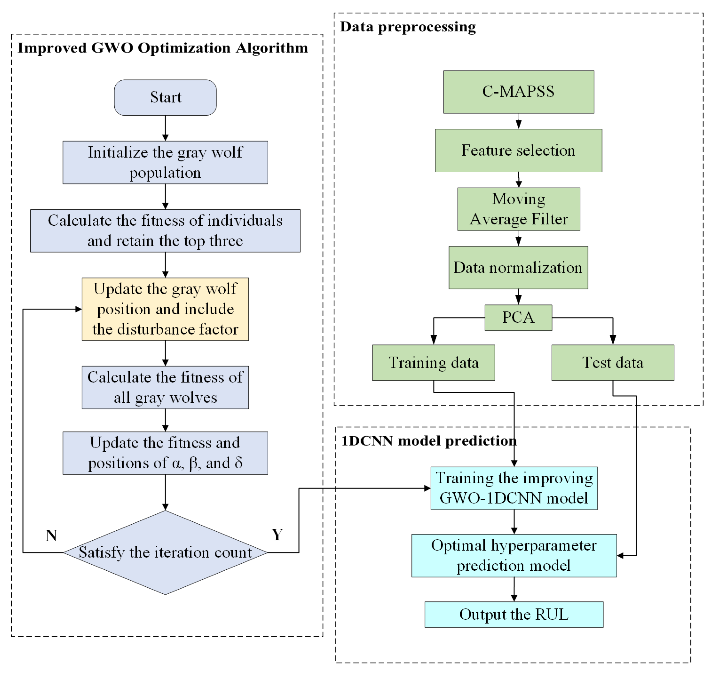
To address the limitations of deep learning models, including the high complexity of hyperparameter space, low efficiency of empirical tuning, and difficulty in achieving optimality, as well as the problem of traditional Gray Wolf Optimizer prone to local convergence, this study proposes a 1D convolutional neural network prediction model improved by a dynamic perturbation factor-based GWO. The model utilizes the improved GWO to perform global optimization on the initial learning rate, regularization parameter, and number of hidden layer neurons of the 1DCNN, and constructs a remaining useful life prediction model for aircraft engines based on the optimal hyperparameters. Figure 3 illustrates the overall workflow of the improved GWO-1DCNN prediction model. The specific steps are as follows:

(1)

Sensor data feature screening was conducted based on visual observation of degradation trends, resulting in the selection of 14 core sensor data metrics with the strongest degradation representation capabilities. The data were then processed using moving average filtering and normalization. Given that the degradation process of aircraft engine sensor data exhibits a low-frequency, slowly varying trend spanning multiple operational cycles with noise dominated by high-frequency random fluctuations, moving average filtering was chosen for data smoothing. This method, which computes the arithmetic mean over a specified time window, inherently acts as a low-pass filter. And the average sliding window size is set to 4 through cross-validation. Its frequency response characteristics align well with the low-frequency components of engine degradation signals, effectively suppressing high-frequency noise while preserving the underlying low-frequency degradation trends. The formula for this process is as follows:

$${\tilde{x}}_t={\displaystyle \frac{x_t+x_{t-1}+\dots +x_{t-K+1}}{K}}$$

(20)

where ${\tilde{x}}_t$ denotes the filtered value at time step $\mathit{t}$, ${\mathit{x}}_t$ represents the measured value at time $\mathit{t}$, and $\mathit{K}$ is the sliding window length. To address the dimensional discrepancies inherent in the multi-source heterogeneous sensor data of aircraft engines, this section describes the data normalization process. Normalization eliminates absolute scale differences between features, enabling parameters with different physical meanings to be compared, assisting the model in better capturing the intrinsic relationships between features, preventing the model from being dominated by numerical magnitudes, and improving prediction accuracy and stability. The Max-Min normalization was adopted for data processing, with its formula as follows:

$$X_{norm}={\displaystyle \frac{X-X_{\min }}{X_{\max }-X_{\min }}}$$

(21)

In this formulation, X_max and X_min are the maximum and minimum values in the original data, and X represents the original data.

(2)

Principal Component Analysis (PCA) was employed to perform dimensionality reduction and reconstruction on the selected 14 features. PCA projects high-dimensional data onto a low-dimensional orthogonal subspace through linear transformation to maximize the variance of the projected data. The core of PCA lies in finding orthogonal principal component directions sorted by variance. When applied to C-MAPSS aircraft engine sensor data, PCA can eliminate linear correlations among sensors (e.g., similar trends among temperature sensors) and fuse related features into independent new features, achieving dimensionality reduction while retaining key information. The core formula is as follows:

$$\mathit{Q}={\displaystyle \frac{1}{n-1}}{\mathit{X}}^T\mathit{X}$$

(22)

$$\mathit{Y}=\mathit{X}\mathit{W}$$

(23)

In this formulation, $\mathit{X}$ denotes the standardized matrix of raw sensor data, where n represents the number of samples. Q corresponds to the covariance matrix of the original dataset, and $\mathit{W}$ constitutes the matrix of eigenvectors associated with the top k eigenvalues of Q. The dimensionality-reduced data is subsequently represented by $\mathit{Y}$. We set a 0.01% information loss threshold as the dimensionality reduction standard, ultimately obtaining eight-dimensional data features that can retain over 99.99% of sensor degradation information.

(3)

By introducing dynamic disturbance factors, improvements are made to the position update process of the GWO algorithm. The improved GWO algorithm is subsequently applied to optimize the hyperparameters of the 1DCNN, leading to the development of an optimal predictive model. The minimal data features obtained are then input into the constructed Remaining Useful Life prediction model to perform forecasts regarding the remaining useful life of the aircraft engine.

(4)

Output the predicted results and conduct a quantitative evaluation of the final results from three aspects—prediction accuracy, error distribution, and lead-lag forecasting scenarios—in order to verify the predictive effectiveness of the proposed model.

4. Experimental Results and Analysis

4.1. Introduction of the Dataset

The acquisition of full-lifecycle monitoring data for aero-engines poses significant challenges in practical experimental settings, primarily stemming from the extended temporal span inherent in degradation processes. The transition from initial healthy states to functional failure typically spans months or even years, rendering comprehensive data collection prohibitively time-intensive and resource-demanding. This challenge is further complicated by stringent industrial safety requirements mandating absolute avoidance of in-service failures. Any operational anomaly or unexpected damage could potentially initiate catastrophic failure chain reactions, thereby fundamentally constraining the accessibility of complete failure progression datasets under real-world conditions [29]. The resultant data scarcity in terminal degradation phases imposes critical limitations on prognostic model validation, necessitating innovative approaches for lifecycle simulation and accelerated degradation testing under controlled environments.

Given the numerous challenges encountered in collecting data from real-world industrial equipment, the majority of current research in this field relies on datasets obtained from accelerated degradation test benches rather than actual operational devices. To facilitate the development of prognostic methodologies, NASA’s Prognostics Center of Excellence (PCoE) has established a Prognostics Data Repository, of which the C-MAPSS Dataset adopted in this study is a representative example. Datasets consist of multiple multivariate time series. Each dataset is further divided into training and test subsets. Each time series is from a different engine, and the data can be considered to be from a fleet of engines of the same type. Each engine starts with different degrees of initial wear and manufacturing variation, which are unknown to the user. This wear and variation is considered normal, i.e., it is not considered a fault condition. There are three operational settings that have a substantial effect on engine performance. These settings are also included in the data. The data is contaminated with sensor noise [30]. Constructed via a high-fidelity gas turbine performance simulation model, this dataset is designed to replicate the progressive performance degradation process of core rotating components—specifically, the fan, Low-pressure Compressor (LPC), High-pressure Compressor (HPC), High-pressure Turbine (HPT), and Low-pressure Turbine (LPT)—under the combined effects of aerodynamic and thermodynamic coupling.

The turbofan engine dataset systematically records full-lifecycle degradation data of engines, which are divided into four distinct subsets (FD001–FD004) based on the complexity of flight operating conditions and the diversity of failure modes. Taking FD001 as an example, it contains complete operation cycle data for 100 engine units, including training samples, test samples, and their corresponding true remaining useful life (RUL) reference values. In the training set, the magnitude of faults progressively increases until system failure, whereas the test set terminates before system failure occurs. The core task of predictive modeling lies in constructing a regression estimation model for remaining useful life, whose mathematical essence is to deduce, from the truncated time-series data in the test set, the number of operational cycles that can be sustained by the engine from the end of observation until functional failure—specifically, how many additional cycles the engine can operate after completing its last recorded cycle. Finally, the predictive performance of the corresponding model is evaluated by comparing the predicted values of the test set with their true values.

An examination of the FD001 data structure reveals that each engine unit is represented as a 26-dimensional feature matrix: the first two columns denote the unit identifier and cycle index; columns 3–5 represent flight condition parameters (including critical variables such as altitude and Mach number); and columns 6–26 correspond to 21 sensor data features, which are real-time thermodynamic state information collected via a distributed sensor network from key engine components. Detailed definitions of the specific parameters—including sensor configurations and monitored parameters for each key component of the turbofan engine—are listed in

Table 1. Sensor data characteristics.

Sensor Serial Number	Measurement Value	Sign Symbol
Sensor 1	Fan Inlet Total Temperature	T2
Sensor 2	LPC Temperature	T24
Sensor 3	HPC Temperature	T30
Sensor 4	LPT Temperature	T50
Sensor 5	Fan Inlet Pressure	P2
Sensor 6	Bypass Delivery Pipe Pressure	P15
Sensor 7	HPC Outlet Total Pressure	P30
Sensor 8	Physical Fan Speed	Nf
Sensor 9	Physical Core Rotation Speed	Nc
Sensor 10	Engine Pressure Ratio	epr
Sensor 11	HPC Outlet Static Pressure	Ps30
Sensor 12	HPT Static Pressure/Fuel Flow Ratio	phi
Sensor 13	Calibrated Fan Speed	NRf
Sensor 14	Calibrated Core Speed	NRc
Sensor 15	Bypass Ratio	BPR
Sensor 16	Oil and Gas Ratio	farB
Sensor 17	Exhaust Valve Thermal Content	htBleed
Sensor 18	Requirement Fan speed	Nf_dmd
Sensor 19	Calibrated Required Fan Speed	PCNfR_dmd
Sensor 20	HPT Coolant Flow Rate	W31
Sensor 21	LPT Coolant Flow Rate	W32

.

From the perspective of data composition, the system primarily collects four categories of fundamental operational parameters: rotational speed of rotating components, fluid medium pressure, fuel supply rate, and operational temperature values. These basic parameters constitute the core observational dimensions for engine health assessment. For instance, changes in rotational speed can serve as an indicator for judging the stability of power output; fluctuations in pressure reflect alterations in airflow dynamics; fuel flow rate correlates directly with combustion efficiency; and abnormal temperature can promptly warn of risks associated with thermal system imbalance. By virtue of its highly representative capability for the degradation process of aviation engines, the dataset is used to validate the effectiveness of the proposed method.

4.2. Establishment of Evaluation Indicators

To comprehensively evaluate the predictive performance of the proposed model and validate the effectiveness of key data processing procedures, this study employs three complementary evaluation metrics: mean absolute error (MAE), root mean squared error (RMSE), and the scoring function proposed by NASA Prognostics Center (score) [31]. These metrics collectively establish a multidimensional assessment framework by quantifying prediction accuracy from distinct perspectives: MAE provides a robust measurement of absolute error magnitude, RMSE emphasizes larger prediction deviations through quadratic weighting, while the NASA score function incorporates engineering applicability considerations through its specialized scaling mechanism. This tripartite evaluation system enables both rigorous mathematical validation and practical relevance assessment for prognostic model development.

The mean absolute error is the average of the absolute differences between predicted values and true values, reflecting the overall level of model prediction accuracy. It is not sensitive to outliers and focuses on assessing average performance under normal operating conditions. Its calculation formula is as follows:

$$MAE={\displaystyle \frac{1}{n}}{\displaystyle \sum _{i=1}^n\left|r_i^{*}-r_i\right|}$$

(24)

Root mean squared error, also known as standard error, enhances the impact of data points with larger deviations on the results by squaring the difference between predicted and actual values in the actual calculation. Therefore, this metric is sensitive to outliers and can reflect the accuracy of prediction results as well as the distribution of errors. Its calculation formula is

$$RMSE=\sqrt{{\displaystyle \frac{1}{n}}{\displaystyle \sum _{i=1}^n{(r_i^{*}-r_i)}^2}}$$

(25)

In addition to prediction accuracy, another key metric that requires significant attention is the predictive lead and lag. Within this research topic, the impact of lagged prediction is notably more severe than that of lead prediction, due to the fact that lagged predictions may cause delays in aircraft maintenance, thereby incurring substantial economic losses. To address this issue, beyond traditional visual analytical methods for results, PHM08 proposes a novel evaluation index—the score function. This metric assigns higher penalty scores to lagged predictions, defined as cases where the predicted remaining useful life exceeds the actual remaining useful life. Through this scoring mechanism, models with stronger lead prediction capabilities can be effectively screened out, serving as the basis for optimizing prediction performance. The formula is as follows:

$$S_i=\left\{\begin{array}{ll}{e}^{(r_i^{*}-r_i)/13}-1,\hfill & r_i^{*}<r_i\hfill \\ e^{(r_i-r_i^{*})/10}-1,\hfill & r_i^{*}>r_i\hfill \end{array}\right.$$

(26)

$$\mathrm{Score}={\displaystyle \sum _{i=1}^n{S}_i}$$

(27)

In the above evaluation metrics, r_i* represents the predicted remaining lifespan of the i-th target device by the model, while r_i represents the true remaining lifespan of the i-th predicted device. The lower the value of each metric, the better the corresponding model’s predictive performance.

4.3. Sensor Feature Selection

Following the basic structural analysis of the dataset, this section conducts a full-dimensional visual analysis of the 21 sensor parameters in the C-MAPSS Dataset. By observing the variation in data characteristics for each sensor with the number of engine operating cycles, sensors are classified and screened based on the trends in their data changes. This process aims to extract effective signals containing degradation feature information, thereby providing reliable data support for the subsequent construction of remaining useful life prediction models.

Through comparative observation of the data curves for each sensor, three primary patterns of data variation can be identified. The first category comprises sensors whose data exhibit a monotonically increasing trend with the number of operating cycles, including Sensors 2, 3, 4, 8, 11, 13, 15, and 17—a total of eight sensors—as illustrated in Figure 4. (To enhance visualization clarity, all sensor data in this study are scaled proportionally to the same range, with the focus on observing their changing trends.) The sensor signals across all 100 engines exhibit consistent monotonic upward trajectories, demonstrating time-dependent escalation of response magnitudes that correlate with prolonged operational duration. This monotonic progression pattern typically signifies cumulative degradation effects in critical engine components, primarily driven by wear-induced surface alterations, cyclic thermal stress accumulation, and other irreversible material deterioration mechanisms. Such parameter drift systematically reflects the progressive deterioration of physical integrity parameters—a critical diagnostic signature of performance degradation in turbomachinery systems. The observed sensor-response coherence across the entire fleet statistically validates these measurements as robust degradation-sensitive indicators. Their intrinsic prognostic relevance stems from the embedded temporal deterioration patterns that encode essential information about failure precursor development. Given this empirically verified diagnostic significance, these sensor streams warrant prioritized retention as key predictive covariates in subsequent machine learning workflows. Systematic preservation and feature engineering of these degradation-sensitive signals will enhance model capacity to capture latent failure dynamics, ultimately improving remaining useful life prediction fidelity for proactive maintenance optimization.

The second category of sensor data exhibits a monotonically decreasing trend with operational cycles, represented by signals from sensors 7, 9, 12, 14, 20, and 21 (six sensors in total, as shown in Figure 5). While opposite in direction to the first category, this decreasing pattern similarly reflects degradation phenomena during engine operation. Specifically, certain monitored parameters gradually decline as components degrade or fluid dynamic states change during engine aging. Systematic comparative analysis across all engine data confirms the consistent reproducibility of this downward trend in all samples, demonstrating high uniformity and stability. These characteristics make such sensors critical indicators for capturing equipment degradation processes, and they are therefore included in the key feature set for subsequent remaining useful life prediction.

In contrast to the aforementioned categories, the third category of sensor data remains essentially constant throughout operational cycles, with signal values showing no significant variations across different engine samples. These signals originate from sensors 1, 5, 6, 10, 16, 18, and 19 (seven sensors in total). The stable response values indicate that the monitored physical quantities either exhibit weak correlation with engine degradation status or were inherently designed to be independent of equipment health conditions. From a feature selection perspective, such data provide limited useful degradation information for remaining useful life prediction, while potentially introducing model noise or reducing training efficiency. Consequently, these seven sensor channels are excluded from subsequent analyses to ensure focus on information that genuinely reflects equipment state evolution.

Based on the above analysis, this section employs a feature selection criterion rooted in degradation trends: retaining a total of 14 sensor parameters from Categories 1 and 2—those exhibiting significant time-varying patterns—and excluding the seven approximately constant parameters in Category 3. This criterion is established through two considerations. On the physical level, sensor parameters with monotonically evolving characteristics directly reflect the engine’s gradual performance degradation process, aligning with the degradation modeling requirements based on physical failure mechanisms. On the data level, time-varying parameters embed system state information that can effectively enhance the model’s capability to characterize degradation trajectories. In contrast, constant parameters, whose information entropy approaches zero, may introduce data redundancy and even lead to model overfitting. Following feature selection, the dimensionality of the original feature space is reduced from 21 to 14 dimensions. This process not only preserves the integrity of key degradation information but also significantly reduces data complexity, laying a solid foundation for subsequent data engineering and modeling prediction tasks.

4.4. Parameter Optimization Range for Prediction Models

The optimization ranges for three hyperparameters are specified in

Table 2. Hyperparameter optimization range.

Parameter	Optimization Range
L2Regularization	[10−4, 10−3]
numHiddenUnits	[10, 800]
InitialLearnRate	[10−3, 10−2]

, with the algorithm iteration count set to ten. Building upon the network architecture proposed in the previous chapter, this framework primarily focuses on optimizing three critical hyperparameters of the 1DCNN model. All remaining empirical network parameters are configured according to established domain-specific research conventions, with detailed specifications provided in

Table 3. Other prediction network parameter settings.

Parameter	Value
maxEpochs	60
miniBatchSize	20
trainingOptions	adam

.

A comprehensive experimental evaluation was conducted by implementing each activation function variant within the 1D-CNN architecture, enabling empirical selection of the optimal nonlinear transformation for subsequent prognostic tasks.

The comparative performance metrics across different activation functions are rigorously documented in

Table 4. Optimization of activation function selection.

Activation Function	RMSE
tanh	21.35
Sigmoid	34.43
Elu	20.01
ReLU	18.44

. The experimental comparison presented in Table 4 reveals that the 1D-CNN architecture incorporating the ReLU activation function achieves superior predictive performance. Consequently, ReLU has been adopted as the activation function of choice for subsequent investigations.

The model optimization and training process is as follows:

(1)

Mean squared error (MSE) is used as the loss function, as the RUL prediction is a regression task:

$$MSE={\displaystyle \frac{1}{n}}{\displaystyle \sum _{i=1}^n{(r_i^{*}-r_i)}^2}$$

(28)

r_i* represents the predicted remaining lifespan of the i-th target device by the model, while r_i represents the true remaining lifespan of the i-th predicted device.

(2)

The Adam optimizer is used for training deep neural networks due to its adaptive learning rate properties.

(3)

The training process includes iterating over the training data to minimize the loss function using backpropagation. A minimum batch size of 20 is chosen for stochastic gradient descent (SGD) optimization. The model is trained for a fixed number of 60 epochs, depending on the convergence state.

(4)

During training, the optimal combination solution of the three parameters (L2Regularization, numHiddenUnits, InitialLearnRate) is found through the improved Gray Wolf Optimization algorithm, thus obtaining models with different parameters. And then the model is evaluated on the validation dataset after each epoch to monitor its performance and to prevent overfitting.

(5)

In the validation dataset, the model that minimizes the loss function is selected as the final model, which is used for the remaining lifespan prediction in the test dataset.

4.5. Experimental Comparative Analysis

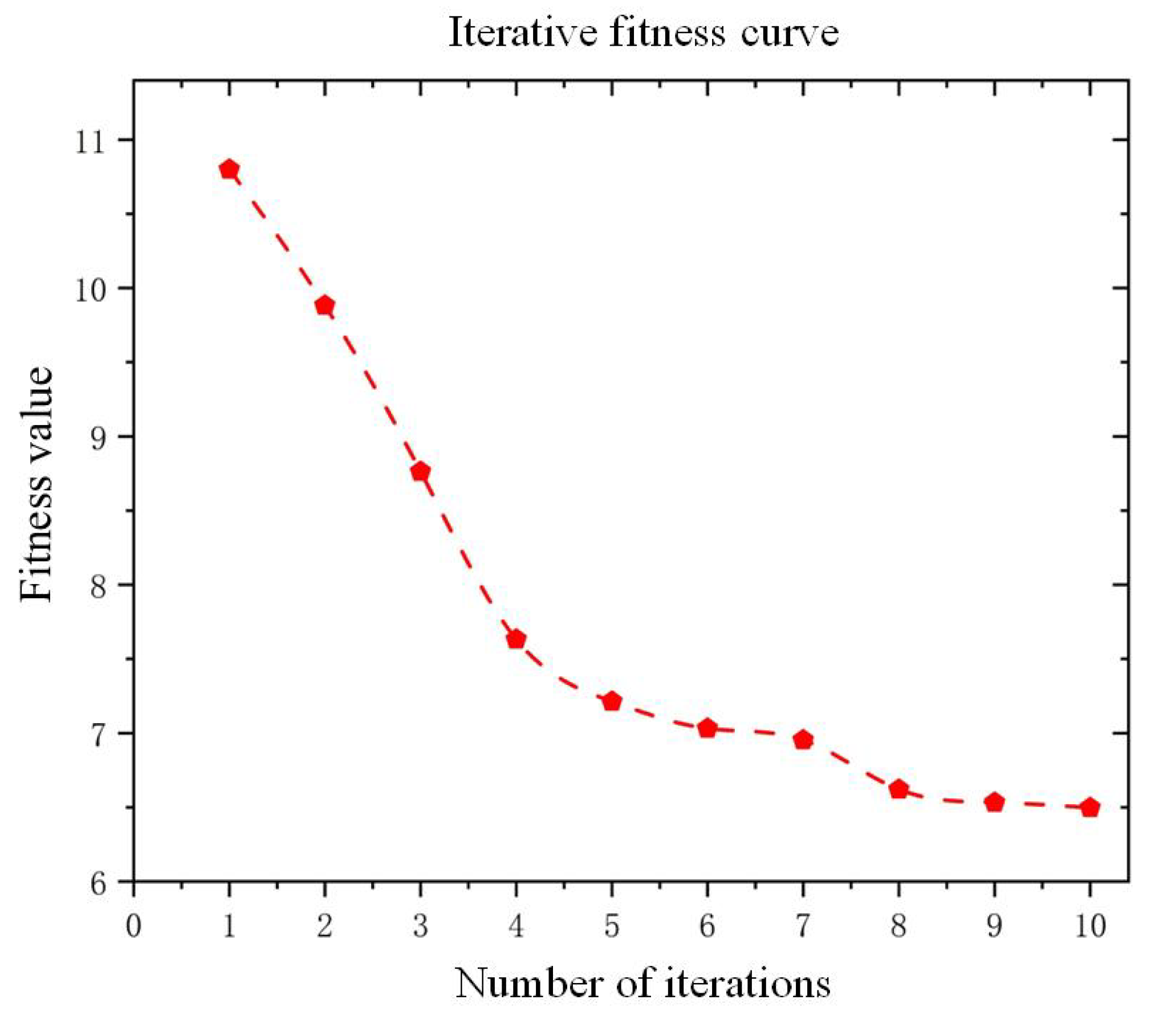
Following the established modeling, the hyperparameter-optimized prediction model was constructed and evaluated using the FD001 dataset. The optimal configuration identified through this process consists of an Initial Learn Rate of 0.00104, num Hidden Units of 524, and L2 Regularization of 0.00059966. Based on five independent model executions with these parameters, the averaged evaluation metrics demonstrate significant performance improvements: mean absolute error (MAE) decreased from 12.56 to 10.14, root mean squared error (RMSE) reduced from 15.32 to 13.76, and the scoring function value improved from 601.20 to 462.91, compared to the non-optimized baseline. The fitness curve of the improved optimization algorithm for the first 10 iterations is shown in Figure 6. From the figure, it can be seen that the proposed method converges quickly. 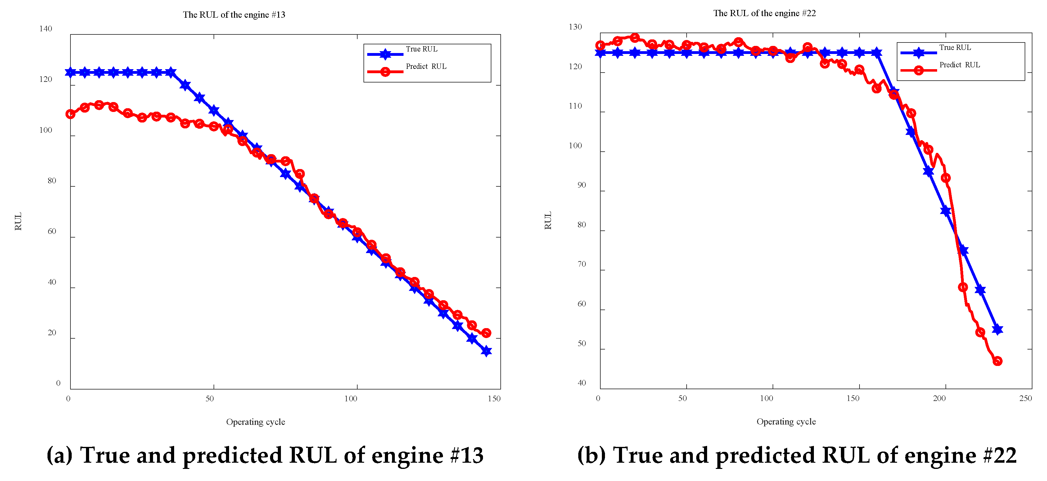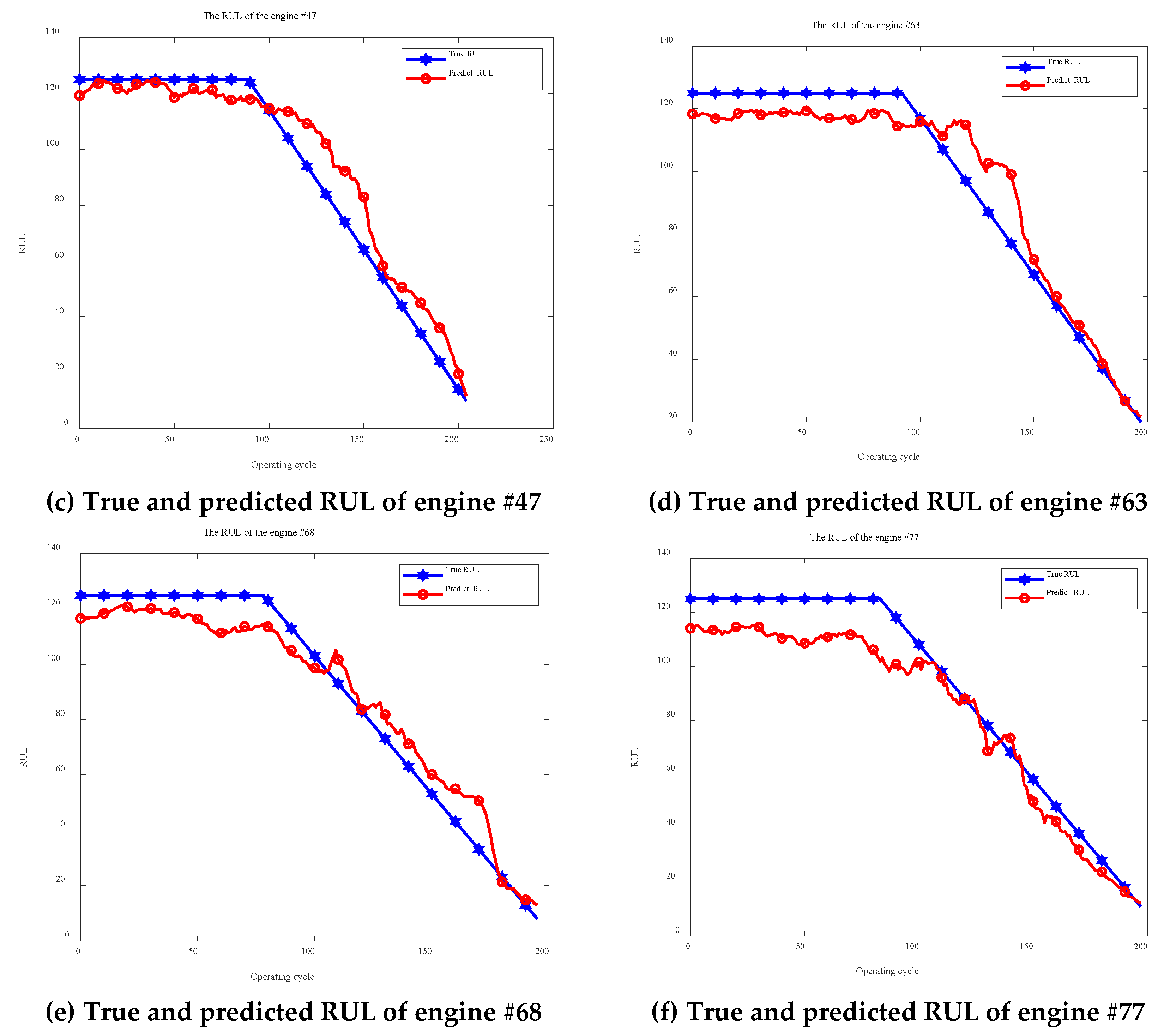Figure 7 presents prediction results for six randomly selected engines, demonstrating the enhanced GWO-1DCNN model’s capability to accurately track actual remaining useful life trajectories while maintaining temporal consistency in degradation pattern recognition. These quantitative and visual validations confirm the effectiveness of the proposed hyperparameter optimization framework in improving prognostic model performance.

The hyperparameter optimization fitness curve demonstrates distinct convergence characteristics of the improved GWO algorithm. During initial iterations, the fitness values exhibit rapid decline, indicating the algorithm’s enhanced global search capability to swiftly identify potential optimal regions. In subsequent iterations, the fluctuation amplitude of fitness values progressively diminishes, ultimately converging to a stable threshold. This behavior validates the balanced coordination between exploration and convergence enabled by the dynamic disturbance factor. The optimization process directly contributes to the precise configuration of model hyperparameters, establishing a robust network foundation for subsequent prediction tasks.

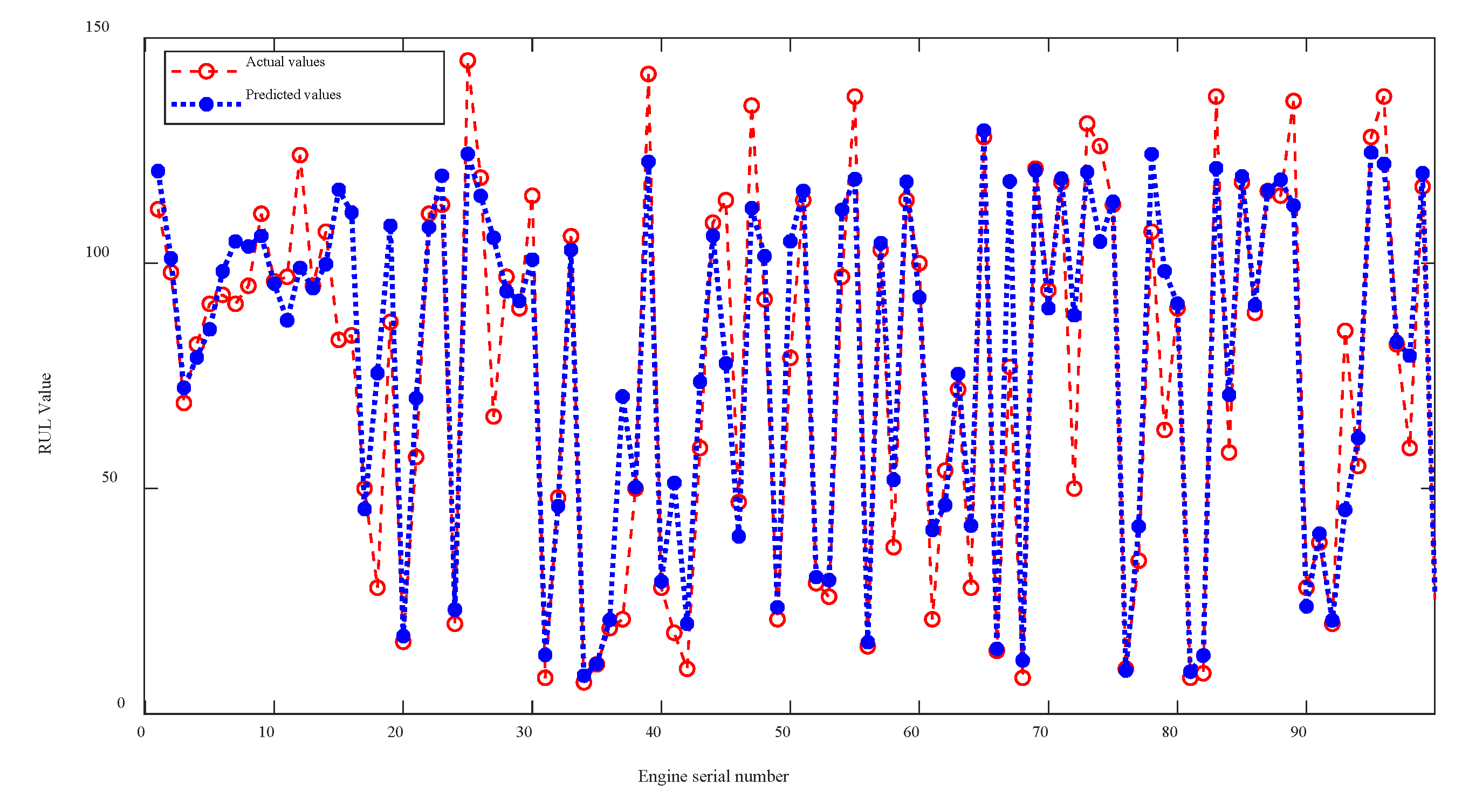
Figure 8 presents the remaining useful life prediction results of the improved GWO-1DCNN model across 100 aero-engines in FD001. The predicted values demonstrate a high degree of consistency with ground truth measurements in overall degradation trajectories, indicating the model’s strong capability in characterizing engine degradation processes. These results validate both the effectiveness of the proposed parameter optimization strategy and the critical role of hyperparameter tuning in improving RUL prediction accuracy. The systematic alignment between predictions and actual degradation patterns confirms the model’s capacity to capture essential failure progression characteristics, establishing its practical utility for aviation maintenance prognostics.

The error distribution of the predictions, as shown in Figure 9, demonstrates that the model exhibits high accuracy and stability in the task of predicting the remaining useful life of aviation engines. Experimental data indicate that the majority of the final RUL prediction errors from the optimized model are concentrated within the range of [−10, 10] cycles, accounting for over 65%—a significant improvement compared to 50% before optimization. Additionally, the frequency of extreme cases where the absolute error exceeds 30 cycles has significantly decreased, fully verifying the reliability of this prediction method.

Figure 10 visualizes the directional distribution of prediction errors, revealing the engineering applicability of the proposed improved GWO-1DCNN model. For the enhanced model, proactive predictions (where actual remaining useful life exceeds predicted values) account for 74% of cases, representing a four-percentage-point improvement over the pre-optimization baseline of 70%. Although this improvement appears relatively modest in magnitude, the overall prediction results maintain a statistically significant proactive bias. This systematic overestimation tendency effectively mitigates operational risks associated with the underestimation of remaining lifespan, thereby enhancing safety assurance in maintenance decision-making processes.

Based on the analysis of the above prediction results, comparative experimental analyses are conducted on three datasets: FD001, FD002, and FD003. The prediction model constructed in this study is compared with the 1DCNN models optimized by three mainstream optimization algorithms, Particle Swarm Optimization and Genetic Algorithm, the GWO-1DCNN prediction model, and the state-of-the-art prediction models, CNN-LSTM and BO-LSTM. This comparison aims to fully demonstrate the advantages of the proposed method in exploring and optimizing the hyperparameter solution space, the improvement in the optimization efficiency of the Gray Wolf Optimizer through the improved strategy incorporating dynamic perturbation factors, and the overall prediction performance of the model. The specific comparison results are presented in

Table 5. Comparison of FD001 forecast indicators.

Predictive Model	MAE	RMSE	Score
PSO-1DCNN [32]	10.84	14.65	493.68
GA-1DCNN [33]	11.37	15.13	554.39
GWO-1DCNN [34]	11.06	14.71	531.62
CNN-LSTM [35]	12.24	14.82	526.40
BO-LSTM [36]	14.02	15.19	611.35
Improved GWO-1DCNN	10.14	13.76	462.91

,

Table 6. Comparison of FD002 forecast indicators.

Predictive Model	MAE	RMSE	Score
PSO-1DCNN	17.53	24.58	8755.30
GA-1DCNN	18.06	25.31	8782.17
GWO-1DCNN	17.82	24.86	8504.55
CNN-LSTM	18.11	24.92	8861.63
BO-LSTM	18.50	25.53	9801.08
Improved GWO-1DCNN	16.22	23.08	8147.36

and

Table 7. Comparison of FD003 forecast indicators.

Predictive Model	MAE	RMSE	Score
PSO-1DCNN	12.68	15.97	672.46
GA-1DCNN	13.10	16.80	780.62
GWO-1DCNN	12.91	16.36	730.91
CNN-LSTM	14.09	16.83	681.49
BO-LSTM	14.52	17.02	851.22
Improved GWO-1DCNN	12.10	15.51	608.35

.

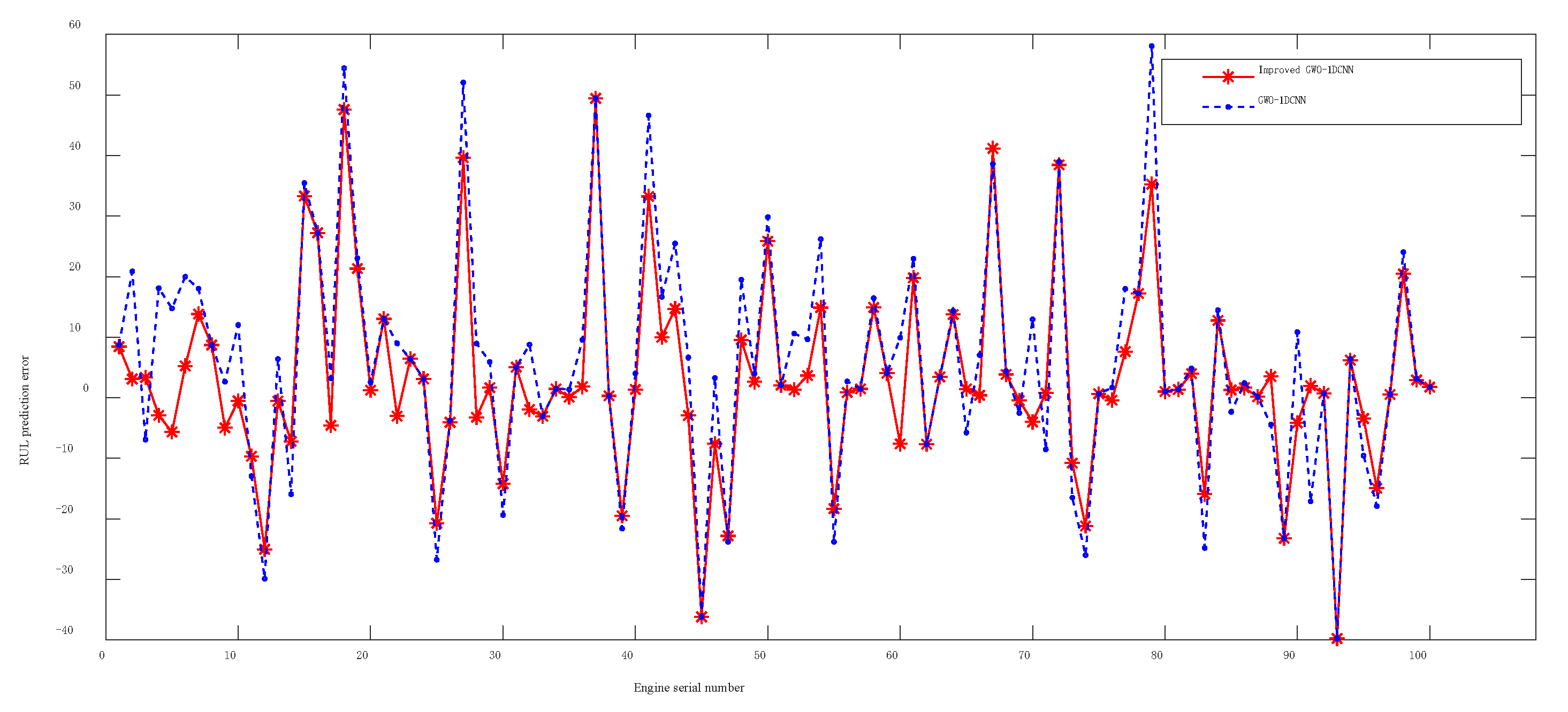
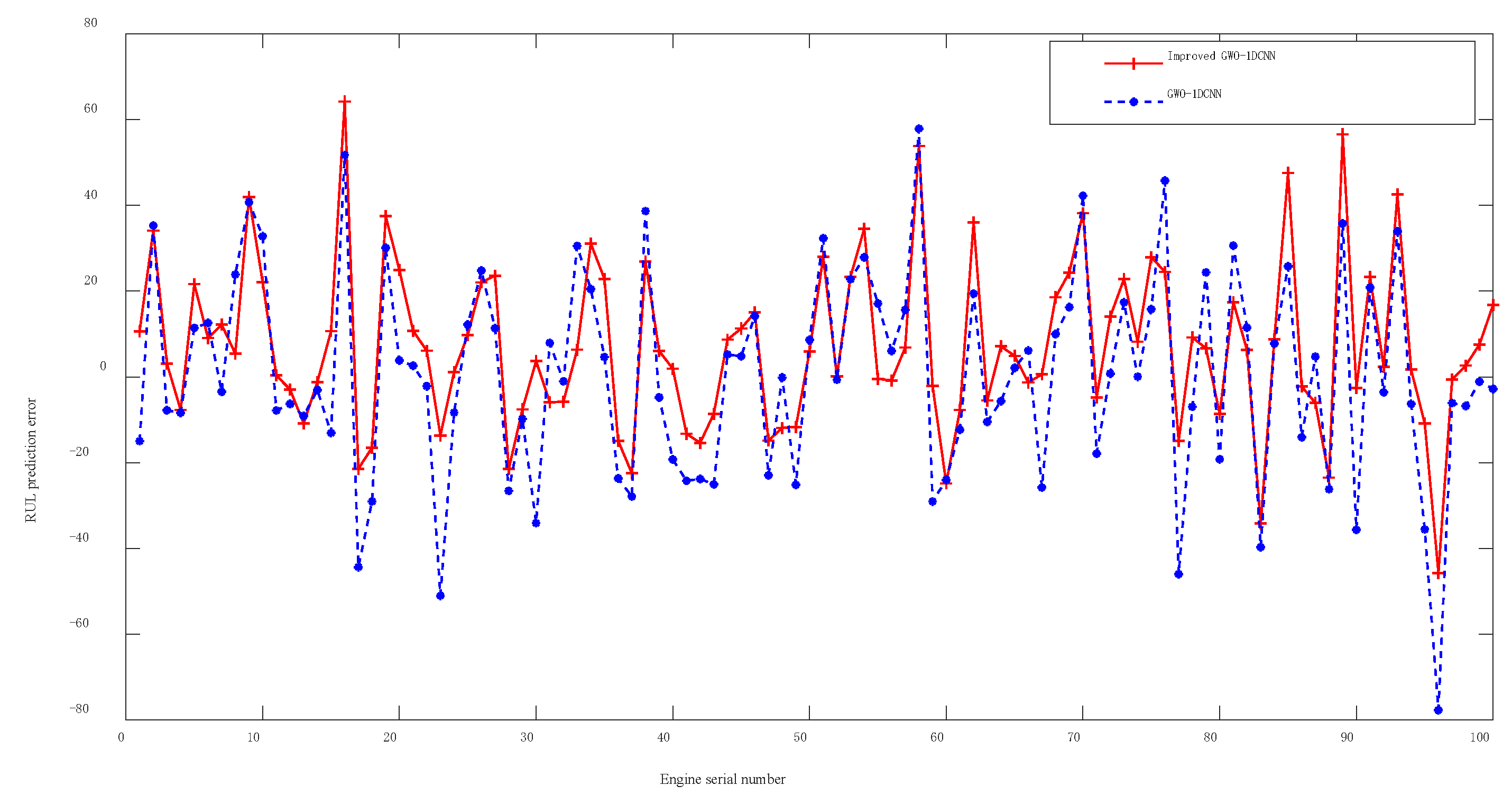
The experimental results indicate that the improved GWO-1DCNN prediction model outperforms the models optimized by the other two algorithms (PSO and GA) with lower values in all three evaluation metrics, highlighting the significant advantages of the proposed method in hyperparameter optimization. Specifically, when compared with the standard GWO-1DCNN, the improved GWO-1DCNN incorporating dynamic perturbation factors achieves average reductions of 8.6%, 7.4%, and 10.1% in mean absolute error, root mean squared error, and score values across the FD001–FD003 datasets, respectively. This demonstrates that the improved strategy effectively mitigates the tendency of the Gray Wolf Optimizer to converge to local optima during position updates, thereby enhancing the quality of optimized hyperparameters. Visual comparisons of prediction errors generated by the models before and after improvement on the FD001–FD003 datasets (as illustrated in Figure 11, Figure 12 and Figure 13) further confirm that the improved GWO-based model exhibits significantly smaller errors and superior prediction performance. Finally, when benchmarked against state-of-the-art methods, the proposed model achieves an 8–10% improvement in all three metrics on the FD003 dataset with complex operational conditions. These results collectively validate the effectiveness and superiority of the improved GWO-1DCNN prediction approach in the field of remaining useful life prediction for aviation engines.

The analysis showed that each method has certain errors, and the main reason is the characteristics of the dataset itself. The data is contaminated with sensor noise. And each engine starts with different degrees of initial wear and manufacturing variation [30]. These increase the difficulty of prediction.

5. Conclusions

This study proposes an enhanced Gray Wolf Optimizer-based one-dimensional convolutional neural network model for predicting the remaining useful life of aviation engines, addressing the challenges of hyperparameter tuning in deep learning and the tendency of the traditional Gray Wolf Optimizer to converge to local optima. The key innovation lies in introducing a dynamic perturbation factor into the Gray Wolf Optimizer, which initially expands the search range to avoid premature convergence and later narrows it for fine-grained optimization. The improved Gray Wolf Optimizer is then applied to optimize the hyperparameters of the one-dimensional convolutional neural network, achieving optimal performance. The optimized model demonstrates significant improvements, yielding a mean absolute error of 10.14, root mean squared error of 13.76, and a score function value of 462.91. Comparative experiments on the FD001–FD003 datasets show that the proposed model outperforms one-dimensional convolutional neural network models optimized by Particle Swarm Optimization and Genetic Algorithm, reducing all error metrics by 6–11%, and surpasses the standard Gray Wolf Optimizer-one-dimensional convolutional neural network by 8.6%, 7.4%, and 10.1% in mean absolute error, root mean squared error, and score values, respectively. Additionally, it achieves average root mean squared error reductions of 9.3% and 7.5% compared to state-of-the-art Bayesian Optimization–Long Short-term Memory and convolutional neural network–Long Short-term Memory models, demonstrating its superior accuracy and reliability in aviation engine remaining useful life prediction. In addition, the proposed method can be applied to the prediction of the lifespan of other equipment and related time series prediction. Particularly when the established model requires hyperparameter optimization, the proposed method and ideas can fulfill these requirements.