Study on Angular Velocity Measurement for Characterizing Viscous Resistance in a Ball Bearing

Abstract

This article describes a machine vision-based method for measuring the angular velocity of a rotating disk to characterize the viscous resistance of a ball bearing. A bright marker was attached to a disk connected to a shaft supported by two ball bearings. Rotation of the marker was recorded with a digital camera. A simple algorithm was developed to track the trajectory of the marker and calculate angular displacement of the disk. For accurate detection of the rotating marker, the algorithm employed Multi-Otsu thresholding and the Least Squares Method (LSM). Verification of the proposed method was carried out through a direct comparison between the predicted rotational speeds and measured ones by a commercial tachometer. It was demonstrated that the percentage error of the proposed method was less than 1.75 percent. The evolution of angular velocity after motor power-off was measured and found to follow an exponential decay law. The exponent was found to remain consistent regardless of the induced rotational speed. This proposed measurement method will offer a simple and accurate non-contact solution for monitoring angular velocity and characterizing the resistance of a bearing.

1. Introduction

The angular velocity of rotating components is one of the important indicators for diagnosing the condition of rotating machinery. By measuring the angular velocity of rotating components such as disks and blades, it is possible to determine angular acceleration, revolutions per minute, and even assess the condition of bearings.

Ball bearings are widely used for supporting a shaft in an electric motor [1]. Oils or greases play a role in minimizing the friction between a ball and a ring. Degradation of lubricants in a bearing leads to increased viscous resistance and friction, which impedes the rotation of the shaft. Under unpowered conditions, viscous resistance and friction are known to be the major factors that reduce the shaft’s rotational speed. That is, the reduction rate of the rotational speed is associated with the resistance (viscous drag and friction) in a ball bearing. Therefore, by measuring the change in rotational speed under unpowered conditions it may be possible to quantify the conditions of a bearing, including lubrication contamination and bearing damage. Vibration-based and acoustic emission-based condition monitoring techniques are being developed to monitor the condition of rolling element bearings [2,3]. These techniques measure vibration and acoustic emissions under normal bearing operating conditions and distinguish them from anomalies. For successful application, external interfering factors such as vibrations from adjacent machinery, ambient noise, and operational noise from the machinery itself must be minimized or filtered out.

Various studies have been carried out on real-time angular velocity measurement methods. Particularly, non-contact angular velocity measurement using machine vision-based techniques is noteworthy. Event-based angular speed measurement utilized event-based vision sensors to determine rotational speed by analyzing the time between detected events [4]. A rotating spot image-based method estimated the angular displacement of a rotating spot disk using machine vision techniques [5]. Monocular vision-based measurement has also been proposed to measure angular rate and acceleration during rotational motion [6]. To improve the accuracy of angular rate estimation, an enhanced line segmentation detector (LSD) with sub-pixel accuracy was applied. In this method, angular velocity was computed based on the angular difference between video frames. Additionally, other research has explored the use of high-speed RGB vision for precise rotor angle measurement [7]. By analyzing a switching RGB pattern on a rotor, the rotation angle was determined at speeds of up to 6000 RPM.

Another approach involves using a high-speed camera [8,9,10]. A linearly varying-density fringe pattern (LVD-FP) and a high-speed camera were used for determining instantaneous rotational speed [8]. A camera-based system that applies image processing techniques such as the Chirp-Z transform and auto-correlation has also been proposed [9]. In this method, an imaging device and a periodicity detection algorithm were developed to measure rotational speed accurately. However, motion burring at high rotational speeds led to a decrease in the accuracy of the angular velocity. Motion blur reduction is one of the key issues for accurate angular velocity measurement. A real-time motion blur compensation system was proposed for high-speed one-dimensional motion between a camera and a target [10]. The system utilized a galvanometer mirror with continuous back-and-forth oscillating motion. Motion blur analysis using polar transformation provided a flexible method for measuring the angular velocity of fast-rotating objects [11]. Non-contact measurement using an electronic rolling shutter camera has also been introduced for measuring extremely high rotational speeds of a propeller [12]. In this method, the geometric distortion of captured frame images, caused by the rolling shutter effect, was analyzed to determine the relationship between angular velocity and image distortion. The rotational Doppler effect was used to detect the rotational velocity of a rough surface [13]. Spectrum analyses using the orbital angular momentum modal expansion method were employed to measure the velocity of a rotational rough surface. However, these methods require expensive equipment and a measurement environment with minimal vibration. In addition, little research has addressed their application to bearing condition monitoring.

This article develops a non-contact measurement method for the angular velocity of a rotating component supported by ball bearings. A machine vision algorithm using a digital camera is proposed. The proposed method is used for measuring rotational speed and for characterizing ball bearing resistance. The algorithm trackchs the centroid trajectory of a bright region attached to a rotating disk. Verification of the proposed method is achieved by direct comparison between calculated and measured revolutions per minute. The evolution of angular velocity after power-off is measured and described using an exponential decay law. The resistance of a ball bearing component is then characterized as a parameter of an exponential decay law.

2. Materials and Methods

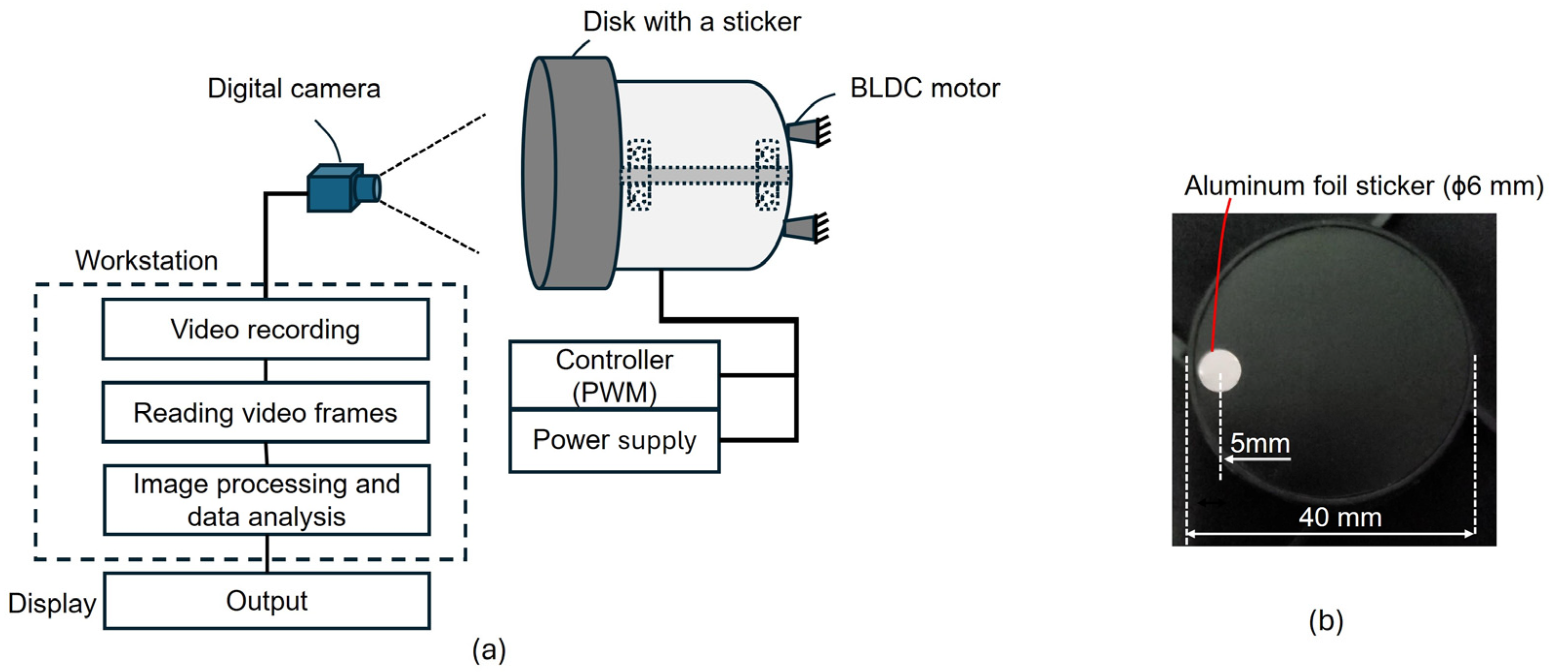
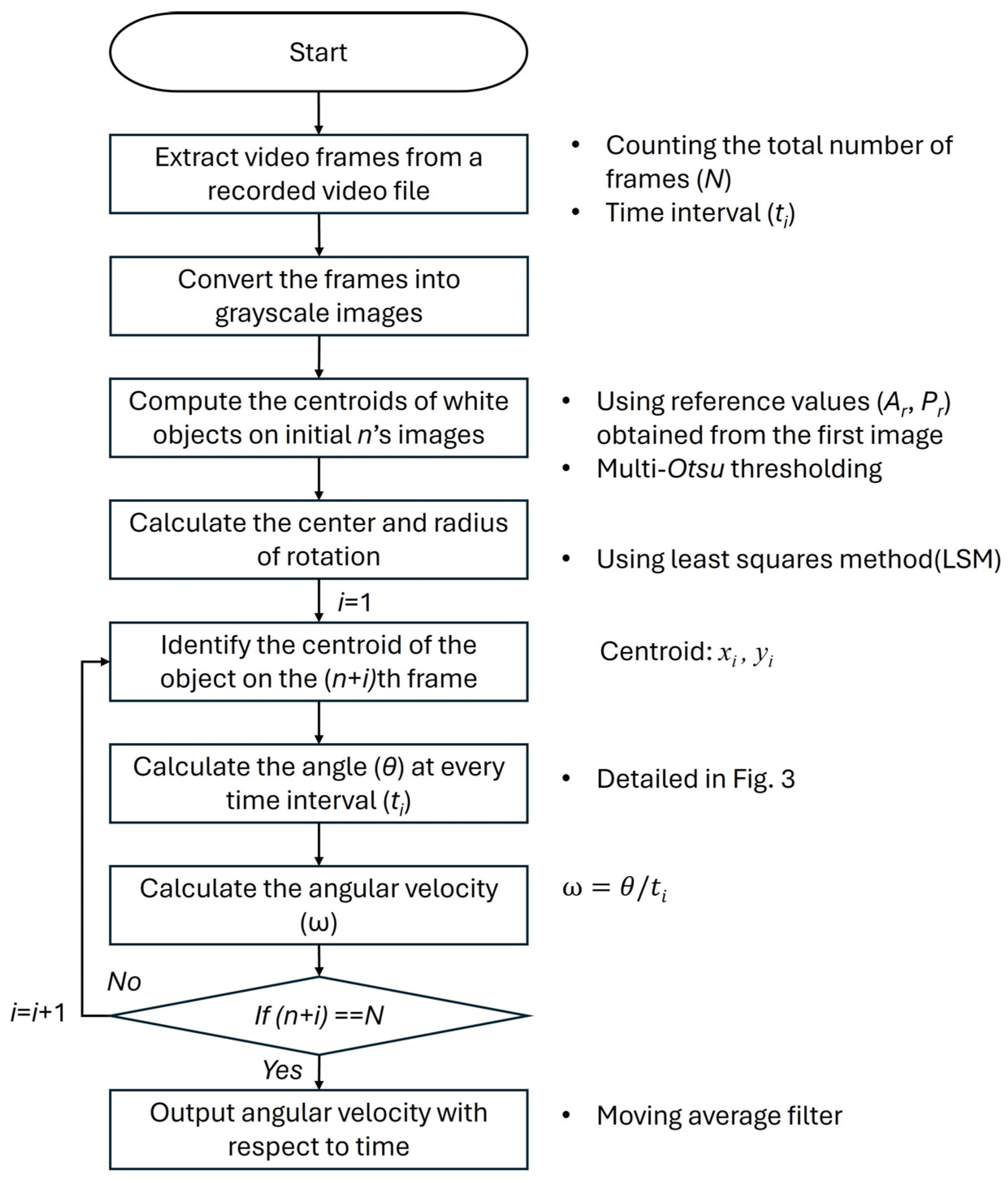
A Proposed Angular Velocity Measuring System

Figure 1 illustrates the proposed system setup for angular velocity measurement using a digital camera. In Figure 1a, the system diagram shows a digital camera positioned to capture the rotation of a disk attached to a BLDC motor (12V DC) containing two ball bearings (PIB Inc., Naperville, IL, USA). Each bearing contains six balls made of AISI440C stainless steel with a diameter of 1.588 mm. Ester oil was applied to a contact surface between the ball and a ring (AISI 440C, (PIB Inc., Naperville, IL, USA)). The motor (Arctic Inc., Florence County, SC, USA) was controlled using a PWM (Pulse-Width Modulation) controller powered by a separate power supply. The digital camera (charge-coupled device, 12 MP, max. frame rate of 240 fps) was connected to a workstation that performed the following three main tasks: video recording, reading video frames, and image processing with data analysis. The processed data (angular velocity and revolutions per minute) was then displayed on a screen. Figure 1b illustrates the design of the rotating disk. It was a circular disk with a diameter of 40 mm, featuring an aluminum foil sticker with a diameter of 6 mm as a marker. The center of the sticker was placed 5 mm away from the edge of the disk. This marker aided in tracking the disk’s rotational motion when recorded by the digital camera, enabling precise image processing and data analysis.

Figure 2 shows a detailed flowchart of the process used to calculate the angular velocity of a rotating object from a recorded video file. This flowchart provides a structured overview of the algorithm used for analyzing rotational motion. The procedure began by extracting individual video frames and counting the total number of frames (N) while noting the time interval (t_i) between them. Here, the time interval was set to be 1/240 s. Each extracted frame was then converted into a grayscale image to simplify further image processing. Using the initial n’s images (e.g., n = 5), white objects were detected by applying Multi-Otsu thresholding [14,15] to each frame, which enables efficient separation of the object from the background. Subsequently, the center and radius of rotation were calculated with n’s centroid points of the detected objects by using the Least Squares Method (LSM). After calculation of the center and radius of rotation, the centroid of the object in each frame was identified (the detail code was presented in Appendix A). In order to predict an angular displacement, it is important to detect the rotating marker accurately. In this article, one object, satisfying the following area (A), perimeter (p), and position conditions, was selected among various objects identified by Multi-Otsu thresholding.

• Condition 1: $0.5<{\displaystyle \frac{A}{A_r}}<1.5$ and $0.5<{\displaystyle \frac{p}{p_r}}<1.5$;
• Condition 2: Among objects satisfying Condition 1, the nearest object to the predicted position (determined with the angular displacement of the previous frame).

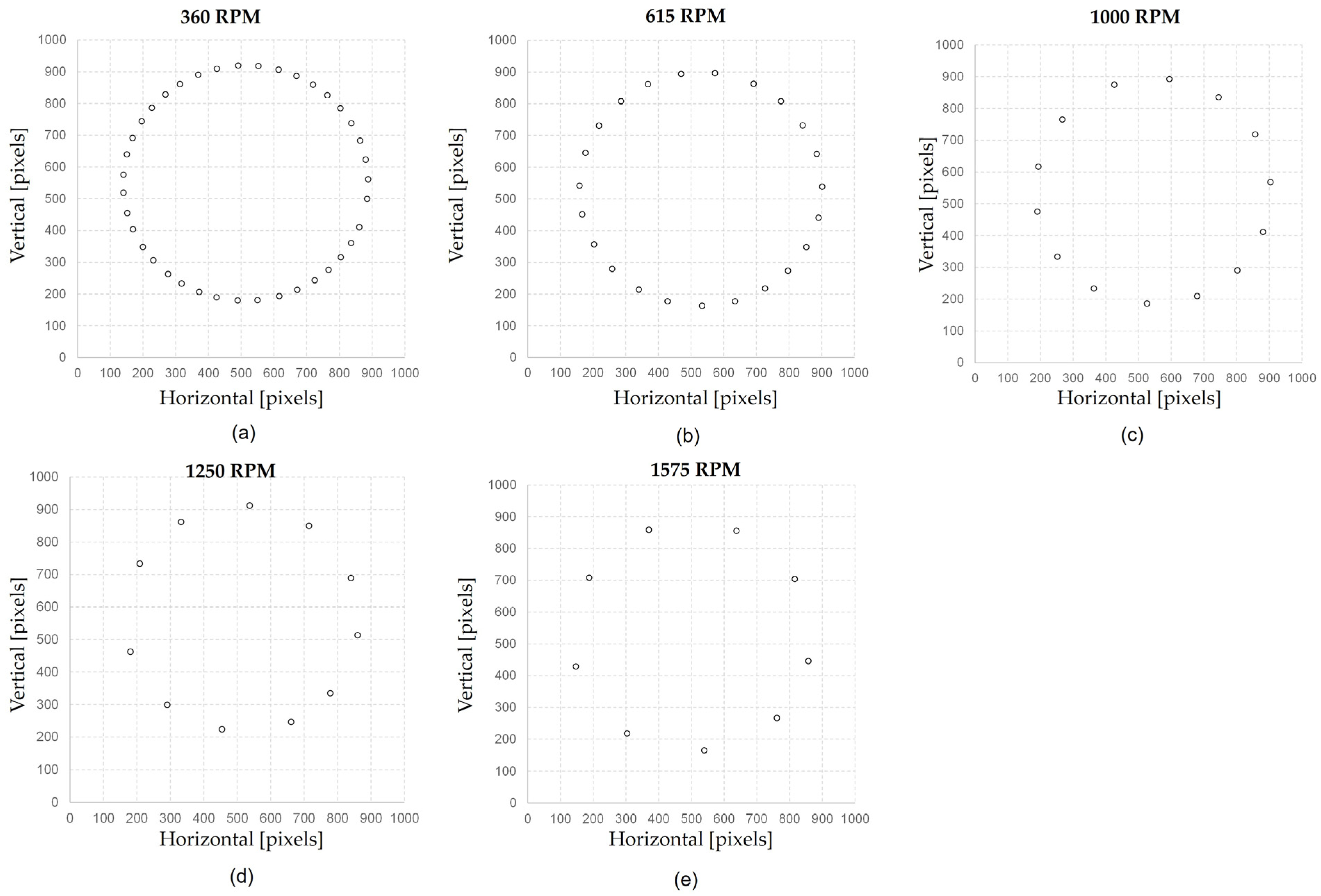
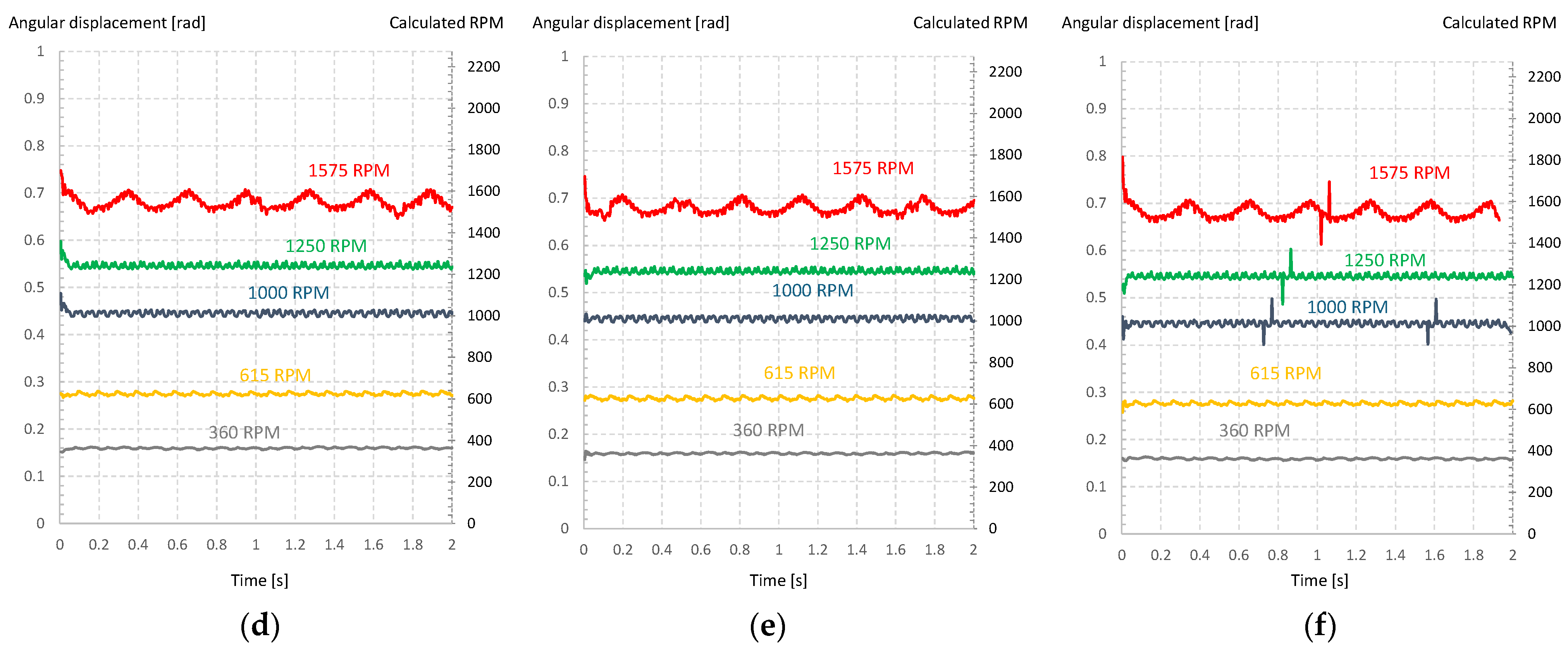
In Condition 1, A_r and P_r denote the reference area and the reference perimeter of a bright object obtained from the first frame, respectively. The angular displacement (θ) at each time interval was then calculated and the angular velocity (ω) was computed. The loop iterated through all frames until the last one was analyzed. Finally, the calculated angular velocity over time was displayed after passing through a ten-point moving average filter.

Figure 3 illustrates the geometric principle underlying the calculation of angular displacement from the tracked centroids. It depicts two consecutive positions of the marker on the rotating disk, represented by coordinates (x_i,y_i) and (x_i−1,y_i−1), corresponding to the current and previous frames, respectively. The center of rotation was marked as O, with the distance from O to each marker position being the constant radius R. The angular displacement (θ) between these two positions was calculated using the chord length formed between them. By applying trigonometry, the half-angle θ/2 was determined using the following formula:

$$\theta =2\times {\mathit{sin}}^{-1}{\displaystyle \frac{\sqrt{{(x_i-x_{i-1})}^2+{(y_i-y_{i-1})}^2}}{2R}}$$

(1)

This equation utilized the distance between the two points as the chord length and divided it by twice the radius to obtain the half-angle using the inverse sine function. This geometric approach enables an accurate and fast calculation of angular displacement, which is then used in the flowchart of Figure 2 to determine angular velocity.

Figure 4 presents a sequence of image processing steps for tracking a rotating disk marker over five frames (a–e) and its corresponding motion trajectory (f). Each frame consists of the following three sections: the grayscale image of the rotating disk, a pixel intensity histogram with Otsu’s thresholding, and the binarized (black-and-white) image highlighting the detected marker. The grayscale images show the bright regions corresponding to circular markers on the rotating disk at five different time steps, while the histograms illustrate pixel intensity distributions used for segmentation. On the binarized images, the centroids of the white regions were clearly shown, confirming successful marker detection. The marker’s detected positions across frames are collectively presented on a single plot (Figure 4f); the labeled positions (1st to 5th) indicate the marker’s movement over time, enabling the calculation of angular displacement. Matlab (2024b) codes for finding the motion trajectory with five positions are detailed in Appendix A.

3. Results

The resistance of a ball bearing can be identified at low rotational speeds. Thus, in this article, angular velocity was measured at speeds of up to 1575 RPM. Figure 5 illustrates the trajectory of a rotating marker at different rotational speeds, ranging from 360 RPM to 1575 RPM. Each of the following subplots (a–e) represent the detected marker positions in a two-dimensional coordinate system for induced RPM: (a) 360 RPM, (b) 615 RPM, (c) 1000 RPM, (d) 1250 RPM, and (e) 1575 RPM. It was identified that the marker positions formed a well-defined circular pattern, indicating clear and consistent detection. At higher rotational speeds, fewer detected markers were observed in a single circular trajectory. Codes for detecting the positions and calculating angular displacement are presented in Appendix B.

Figure 6 presents a time-series plot illustrating angular displacements in radians (left vertical axis) and the corresponding calculated RPM (right vertical axis) over a duration of two seconds. Five distinct revolutions per minute (360 RPM, 615 RPM, 1000 RPM, 1250 RPM, and 1575 RPM) were represented using different colors. The plot shows that lower speeds (360 RPM and 615 RPM) maintained relatively stable angular displacements with minimal fluctuations. This fluctuation may be associated with inherent properties of the electric motor used and the mechanical boundary condition securing the motor.

Table 1. Measurements of revolutions per minute. Standard error was defined as the standard deviation divided by the square root of the number of measurements.

Index	Tachometer * [RPM]	Measurement, Average for Two Seconds, RPM						Average	Standard Error
		No. 1	No. 2	No. 3	No. 4	No. 5	No. 6
1	360	364	363	364	363	362	362	362.9	0.38
2	615	619	619	621	624	627	628	623.0	1.64
3	1000	1021	1023	1023	1013	1013	1012	1017.5	2.21
4	1250	1248	1249	1242	1241	1239	1239	1242.9	1.74
5	1575	1567	1571	1567	1549	1546	1544	1557.4	4.99

* Tachometer: non-contact digital measurer (sampling rate of 1 time per second) with accuracy of ±2.6 RPM at lower than 1000 RPM and ±15 RPM at higher than 1000 RPM.

shows the average values of RPM values found in Figure 6. The average of six measurements was presented along with the standard error. As shown in the table, the maximum standard error was found to be 4.99.

Table 2. Direct comparison between non-contact tachometer values and predicted ones.

Index	Tachometer [RPM]	Predicted RPM, Average	Percentage Error [%]
1	360	362.9	0.81
2	615	623.0	1.30
3	1000	1017.5	1.75
4	1250	1242.9	0.57
5	1575	1557.4	1.12

shows a direct comparison between calculated RPM values and measured ones by a non-contact tachometer. There were small errors between the two values (less than 1.75 percent). Note that the percentage error was defined as the absolute value of the difference between the measured and the calculated RPM divided by the measured value and multiplied by 100. Table 2 demonstrates that the proposed method can measure revolutions-per-minute with less than a 1.75 percent error within the chosen range.

When motor power is removed from a rotating disk, rotating speed is reduced, and the disk comes to a stop due to viscous resistance and the frictional forces of a ball bearing. For the purpose of describing the resistance phenomenon, the power of a driven electric motor was removed. Figure 7 presents a time-series plot of angular velocity, measured in radians per second (rad/s), and the corresponding calculated revolutions per minute (RPM). The x-axis represents time in seconds, while the left y-axis denotes angular velocity in rad/s, and the right y-axis represents the equivalent RPM. Multiple curves, distinguished by color, indicate the following different initial RPM values: 1575 RPM (red), 1250 RPM (green), 1000 RPM (blue), 615 RPM (black), and 360 RPM (gray). At two seconds, motor power was off. Each curve exhibited an initial steady-state angular velocity followed by a sharp decline around the 2 s mark due to power-off. After this point, the curves showed oscillatory behavior as they gradually approached zero velocity. Below 250 RPM, oscillation of angular velocity seems to be associated with cogging torque effect [16].

In order to describe the decay behavior of angular velocity after motor power cut-off, the exponential decay law was applied to the angular velocity evolutions presented in Figure 7. The following Equation (2) shows the exponential decay law, which is a function of time (t):

$$w\left(t\right)=w_0\times e^{-\beta ·t}$$

(2)

where β is resistance (damping) coefficient, related to condition of a ball bearing component in a BLDC motor, and w₀ denotes the angular velocity at power-off. Equation (1) can be rewritten as the following Equation (3) on the log–linear scale:

$$\ln \left(w\right)={\mathit{ln}(w}_0)-\beta ·t$$

(3)

Figure 8 shows angular velocity evolutions of three different initial rotational speeds on the semi-log scale, consisting of three subplots labeled (a), (b), and (c). Angular velocity values within a range from 31.4 rad/s (300 RPM) to 104.7 rad/s (1000 RPM) were used for excluding oscillatory behavior due to cogging torque. Each subplot shows experimental data as black circular markers and an exponential decay fit as a red curve. The corresponding mathematical expressions of the exponential decay, along with their coefficients and decay rates, were provided in each subplot. The equations indicate that the angular velocity followed an exponential decay trend, with high reported quality of fit (R) values close to 0.99 suggesting a strong correlation between the experimental data and the fitted model. The exponents, β, were close to each other since the evolutions were obtained from the same rotating system containing undamaged ball bearings. The exponent might be used as an indicator for representing the state of a ball bearing. The exponential decay of the angular velocity after power-off could occur due to energy dissipation from various factors such as frictional forces, electromagnetic damping, or viscous drag.

In this article, the maximum rotational speed was 1575 revolutions per minute. This may be included in the low-RPM range for an electric motor. To extend the applicability of the proposed method to fast-rotating components, higher rotational speeds will need to be induced. At high rotational speeds, motion blur becomes severe, as shown in Figure 9c, leading to difficulty in detecting the white area. In this proposed method, Otsu thresholding was applied to each grayscale image. Two threshold levels were automatically determined, and the larger of the two was selected to separate the white region from the background. For accurate detection of the rotating marker, it is important to segment the blurred marker area from other objects caused by variations in lighting and image noise. Therefore, future work should focus on the precise detection of blurred regions. The surface of the tested disk was dark and planar; therefore, the proposed method needs to be improved for high-reflection materials and more complex geometries, such as those of non-planar surfaces of rotors and blades. To use the system as a tool for the predictive monitoring or maintenance of rotating components, it is necessary to evaluate its feasibility in various environments, including variable lighting, vibration, and background noise conditions. The non-contact digital measurer displays the average RPM measured over one second and inherently contains measurement error. Thus, a direct comparison with another measurement method (e.g., a contact-type tachometer) will be helpful for evaluating the proposed method. Additionally, for increasing measurement accuracy, other methods including edge detection and template matching need to be taken into account. In the exponential decay law for bearings, factors such as operating temperature and dynamic loads (e.g., radial or axial forces) need to be considered.

4. Conclusions

This article proposed and validated a machine vision-based method for measuring the angular velocity of a rotating disk driven by a BLDC motor. The trajectory of a bright marker attached to the disk was tracked by using a digital camera. The algorithm for tracking the centroid of a bright region was developed, employing Multi-Otsu thresholding and the Least Squares Method (LSM). Angular displacement was determined with centroids tracked. A direct comparison was carried out between calculated RPM values and measured ones by a non-contact tachometer. It was identified that the percentage error was less than 1.75 percent.

This article analyzed the evolution of angular velocity after power-off, following the exponential decay law, which allowed for the characterization of the resistance in a ball bearing. The exponent in the exponential decay law was found to be constant without regard for the induced rotational speed. It means that the exponent could be used as an indicator to represent the condition of a ball bearing. The exponent is expected to vary with the degradation of the ball bearing. Thus, further work will include the fatigue testing of ball bearings to identify changes in the exponent.

In this article, the maximum value of the induced rotational speed was 1575 revolutions per minute. This may be within the low-RPM range of an electric motor. Thus, it is necessary to apply the proposed method to the high rotational speeds of an electric motor (e.g., greater than 2000 RPM). At high rotational speeds motion blur occurs, which reduces detection accuracy. Therefore, future work should focus on improving the algorithm for high rotational speeds.

References

1. Huang, G.; Lei, W.; Dong, X.; Zou, D.; Chen, S.; Dong, X. Stage-Based Remaining Useful Life Prediction for Bearings Using GNN and Correlation-Driven Feature Extraction. Machines 2025, 13, 43. [Google Scholar] [CrossRef]
2. Doğan, B.K.; Karaçay, T. Temperature and vibration condition monitoring of a polymer hybrid ball bearing. J. Vib. Eng. Technol. 2022, 10, 2385–2390. [Google Scholar] [CrossRef]
3. Mokhtari, N.; Pelham, J.G.; Nowoisky, S. Friction and wear monitoring methods for journal bearings of geared turbofans based on acoustic emission signals and machine learning. Lubricants 2020, 8, 29. [Google Scholar] [CrossRef]
4. Azevedo, G.O.D.A.; Fernandes, B.J.T.; Silva, L.H.D.S.; Freire, A.; de Araújo, R.P.; Cruz, F. Event-based angular speed measurement and movement monitoring. Sensors 2022, 22, 7963. [Google Scholar] [CrossRef] [PubMed]
5. Zhang, F.; Wang, L.; Zhang, J. A visual-based angle measurement method using the rotating spot images: Mathematic modeling and experiment validation. IEEE Sens. J. 2021, 21, 16576–16583. [Google Scholar] [CrossRef]
6. Yang, M.; An, H.; Mo, S.; Gong, H.; Dong, B.; Chen, G. Efficient monocular vision method used for measuring the angular rate and acceleration in rotation motion. Opt. Express 2022, 30, 45436–45446. [Google Scholar] [CrossRef] [PubMed]
7. Kim, H.; Yamakawa, Y.; Senoo, T.; Ishikawa, M. Visual encoder: Robust and precise measurement method of rotation angle via high-speed RGB vision. Opt. Express 2016, 24, 13375–13386. [Google Scholar] [CrossRef] [PubMed]
8. Zhong, J.; Zhong, S.; Zhang, Q.; Peng, Z.; Liu, S.; Yu, Y. Vision-based measurement system for instantaneous rotational speed monitoring using linearly varying-density fringe pattern. IEEE Trans. Instrum. Meas. 2018, 67, 1434–1445. [Google Scholar] [CrossRef]
9. Wang, T.; Wang, L.; Yan, Y.; Zhang, S. Rotational speed Measurement using a low-cost imaging device and image processing algorithms. In Proceedings of the IEEE International Instrumentation and Measurement Technology Conference (I2MTC), Houston, TX, USA, 14–17 May 2018; pp. 1–6. [Google Scholar] [CrossRef]
10. Hayakawa, T.; Watanabe, T.; Ishikawa, M. Real-time high-speed motion blur compensation system based on back-and-forth motion control of galvanometer mirror. Opt. Express 2015, 23, 31648–31661. [Google Scholar] [CrossRef] [PubMed]
11. Altmann, B.; Pape, C.; Reithmeier, E. Determining angular velocities of fast rotating objects based on motion blur to control an optomechanical derotator. Proc. Appl. Math. Mech. 2018, 18, e201800092. [Google Scholar] [CrossRef]
12. Zhao, Y.; Li, Y.; Guo, S.; Li, T. Measuring the angular velocity of a propeller with a video camera using electronic rolling shutter. J. Sens. 2018, 2018, 1037083. [Google Scholar] [CrossRef]
13. Quan, S.; Chen, L.; Wu, S.; Zhang, B. Vectorial doppler complex spectrum and its application to the rotational detection. Appl. Phys. Express 2023, 16, 042002. [Google Scholar] [CrossRef]
14. Otsu, N. A threshold selection method from gray level histograms. IEEE Trans. Syst. Man Cybern. 1979, 9, 62–66. [Google Scholar] [CrossRef]
15. Kim, K. Development of a machine vision system for the average roughness measurement of shot- and sand-blasted surfaces. Lubricants 2024, 12, 339. [Google Scholar] [CrossRef]
16. Islam, M.S.; Mir, S.; Sebastian, T. Issues in reducing the cogging torque of mass-produced permanent-magnet brushless DC motor. IEEE Trans. Ind. Appl. 2004, 40, 813–820. [Google Scholar] [CrossRef]
Figure 1. Schematic diagram of (a) an angular velocity measuring system and (b) the dimensions of a disk and a marker (aluminum foil sticker).
Machines 13 00578 g001
Figure 2. Flowchart for predicting the angular velocity (ω).
Machines 13 00578 g002
Figure 3. Geometric principle for calculating an angular displacement (θ).
Machines 13 00578 g003
Figure 4. Sequence of image processing steps for tracking a marker on a rotating disk. (a) The first, (b) the second, (c) the third, (d) the fourth, and (e) the fifth position. (f) Corresponding motion trajectory. The blue and the red lines represent the first and the second thresholds, respectively.
Machines 13 00578 g004
Figure 5. The centroid trajectory of a bright region for one revolution. (a) 360 RPM, (b) 615 RPM, (c) 1000 RPM, (d) 1250 RPM, and (e) 1575 RPM. Note that the time interval was 1/240 s. The small circle presents the centroid of a detected region.
Machines 13 00578 g005
Figure 6. Angular displacement evolutions (left vertical axis) with respect to time and corresponding RPM (right vertical axis). (a) Measurement No. 1; (b) measurement No. 2; (c) measurement No. 3; (d) measurement No. 4; (e) measurement No. 5; (f) measurement No. 6.
Machines 13 00578 g006aMachines 13 00578 g006b
Figure 7. Angular velocity evolutions after motor power-off.
Machines 13 00578 g007
Figure 8. Angular velocity evolution after power cut-off of a BLDC motor on semi-log scale. (a) 1000 RPM, (b) 1250 RPM, and (c) 1575 RPM. A red line is a fitted curve and dark circles are measured data. The data within the range from 300 to 1000 RPM was selected.
Machines 13 00578 g008
Figure 9. Motion blur phenomenon with respect to rotational speed. (a) 360 RPM, (b) 1575 RPM, and (c) 4000 RPM.
Machines 13 00578 g009