Power Control and Voltage Regulation for Grid-Forming Inverters in Distribution Networks

Abstract

This paper proposes a robust voltage control strategy for grid-forming (GFM) inverters in distribution networks to achieve power support and voltage optimization. Specifically, the GFM control approach primarily consists of a power synchronization loop, a voltage feedforward loop, and a current control loop. A voltage feedforward control circuit is presented to achieve error-free tracking of voltage amplitude and phase. In particular, the current gain is designed to replace voltage feedback for improving the current response and simplifying the control structure. Additionally, in order to optimize voltage and improve the power quality at the terminal of the distribution network, an optimization model for distribution transformers is established with the goal of the maximum qualified rate of the load-side voltage and minimum switching times of transformer tap changers. An enhanced whale optimization algorithm (EWOA) is designed to complete the algorithm solution, thereby achieving the optimal system configuration, where an improved attenuation factor and position updating mechanism is proposed to enhance the EWOA’s global optimization capability. The simulation results demonstrate the validity and feasibility of the proposed strategy.

1. Introduction

In recent years, with improving production and living standards, the electricity demand has increased significantly [1]. The prolonged operation of high-power loads results in increasingly severe voltage quality issues at the terminals of distribution networks [2,3,4]. The extensive integration of power electronic devices has introduced substantial changes to system characteristics, including weakened voltage support performance, reduced system inertia, and diminished frequency regulation capability [5]. Hence, voltage management of distribution networks has garnered widespread attention from experts worldwide [6,7,8]. The low-voltage distribution network is characterized by a long radius, scattered power supply and loads, small line diameter, pronounced seasonality, and insufficient reactive power. These features can lead to voltage drop and a decline in power quality under heavy load conditions [9]. Moreover, the substandard voltage would also adversely affect the safe and stable operation of power equipment and their service life [10].

With the limitations of synchronous generators, traditional distribution networks are gradually transitioning to electronic power systems [11,12,13]. The grid-connected converter technique, particularly the grid-forming (GFM) inverter technique, has emerged as a promising solution to enhance the stability and resilience of modern power systems [14,15,16]. The GFM inverter is controlled as a voltage source, which achieves control objectives by generating the output voltage amplitude and phase reference. The structure of the control module primarily consists of power control and voltage control. The power control aims to achieve grid power synchronization by emulating the power characteristics of synchronous generators, thereby generating the voltage magnitude and frequency reference [17]. The voltage control determines the pulse width modulation voltage reference [18].

Extensive research has been conducted on control strategies for GFM inverters [19,20,21]. To analyze the stability of GFM inverters at the intersection of unsaturated and saturated power angle curves during mode transitions, Yang et al. [22] designed a state-switching model via constant voltage control and proposed a global stability methodology based on Lyapunov theory. Given the advantages of virtual synchronous generators (VSGs), such as inertial support, flexibility, and controllability, a VSG-based grid-connected control strategy for GFM inverters was proposed in [23] to enhance transient angle stability, thereby maintaining the stable operation of the grid. In [24], an automatic coordinated secondary control strategy was proposed for GFM inverters to attain voltage recovery, power distribution, and reactive circulating current attenuation. This strategy utilizes a leader–follower consensus structure, eliminating reliance on centralized controllers and grid support. In addition, information security plays a vital role in ensuring the stable operation of the distribution network. Considering the security of the private information for an individual GFM inverter, Du et al. [25] presented an average-observer-based distributed control scheme to facilitate information exchange while protecting privacy. However, it cannot accelerate current response due to the absence of a current regulation loop.

To address the issue of low voltage at the terminal of distribution networks, voltage regulation is imperative [26]. Significant theoretical research and engineering practices have been conducted both domestically and internationally, yielding notable results [27,28]. In [29], a composite voltage control scheme was proposed to improve the voltage profile of distribution networks and mitigate voltage fluctuations. However, this method necessitates additional consideration of the number of transformer tap operations. Moreover, the user power demand can be managed by controlling the feeder voltage, which can coordinate with the GFM inverter [30]. To cope with permanent fault events, a novel mixed program model was developed to achieve optimal restoration of distribution networks in [31]. Moreover, the model takes into account voltage control devices, such as on-load tap changers in substations. While this method has certain applicability, its economy needs to be improved under overloading conditions. To manage frequent and large-scale voltage fluctuations in distribution networks, Yang et al. [32] introduced a deep reinforcement learning-based dual-time scale voltage optimization scheme by incorporating the data-driven algorithm with physical information. However, it involves high investment costs and exhibits suboptimal reactive power compensation. For distribution network reconfiguration, an effective optimization framework was developed to enhance grid voltage distribution and minimize power loss in [33], in which a Harris hawks optimization algorithm was employed to achieve a globally optimal configuration.

In this paper, a robust voltage control strategy is proposed for GFM inverters in distribution networks to provide power support and enhance low-voltage governance. The main contributions of this work are summarized as follows:

• A GFM control approach is developed, including a power synchronization loop, a voltage feedforward loop, and a current control loop, which enhances terminal voltage quality and provides power compensation. Compared with double-loop control methods [12,14,18,21,23], the proposed approach simplifies the controller structure and improves the flexibility of combining the three control loops.
• An enhanced whale optimization algorithm (EWOA) is proposed to solve the distribution network optimization model with an adaptive attenuation factor and position updating mechanism, which improves the convergence rate and accuracy of the algorithm and avoids the algorithm falling into a local optimum.
• The effectiveness of the proposed scheme is validated through simulation cases. The results demonstrate that the proposed scheme achieves reliable voltage governance and power compensation, and has plug-and-play capability and fast dynamic response.

The rest of this article is organized as follows. The system description and problem statement are outlined in Section 2. Section 3 provides the proposed vector voltage control approach. The simulation results are exhibited in Section 4. Finally, Section 5 comprises the conclusion.

2. System Description and Problem Statement

The schematic diagram of the low-voltage distribution network is displayed in Figure 1. $u_0$ and $u_1$ denote the high voltage side voltage and low voltage side voltage of 10 kV distribution transformer, respectively. $u_2$ denotes the terminal voltage of the distribution network. $R_g+j{X}_g$ denotes the feed line impedance. $P_g+j{Q}_g$ and $P_{\mathrm{L}}+j{Q}_{\mathrm{L}}$ indicate the grid transmission power and the load power, respectively. The subscript $dq$ indicates a $dq$-axis vector of the synchronous $dq$ coordinate system. From Figure 1, the voltage transmission loss can be described as $△u=△U+j\underline{\delta }U=(P_{\mathrm{L}}{R}_g+Q_{\mathrm{L}}{X}_g)/u_2+j(P_{\mathrm{L}}{X}_g+Q_{\mathrm{L}}{R}_g)/u_2$. Moreover, since the phase variation in electric energy is relatively small in the transmission process, the transverse component of the voltage loss can be ignored. Thus, there are the following mathematical relationships [27]:

$$\begin{array}{cc}\hfill & u_1={\displaystyle \frac{u_0}{k_1}},u_2=u_1-{\displaystyle \frac{P_g{R}_g+Q_g{X}_g}{u_1}},\hfill \end{array}$$

(1)

$$\begin{array}{cc}\hfill & P_g={\displaystyle \frac{(u_1{u}_{2}cos\delta -u_2^2)cos\phi +u_1{u}_{2}sin\delta sin\phi }{R_g+j{X}_g}},\hfill \end{array}$$

(2)

$$\begin{array}{cc}\hfill & Q_g={\displaystyle \frac{(u_1{u}_{2}cos\delta -u_2^2)sin\phi +u_1{u}_{2}sin\delta cos\phi }{R_g+j{X}_g}},\hfill \end{array}$$

(3)

where $k_1$ is the transformation ratio of the distribution transformer, $\delta$ is the power angle, and $\phi$ is the impedance angle.

It can be noted that the reactive power compensation should be carried out while compensating for the load voltage to reduce the transmission loss on the line. The reactive powers of the upper feeder and the main transformer are restricted by the reactive power at the terminal of the distribution network; the regulating rule of the reactive power is therefore from the load to the upper level [30]. The voltage at the terminal of the distribution network is constrained by the voltage of the feeder and the upper level, so the regulating principle of the voltage is from the upper level to the load [9].

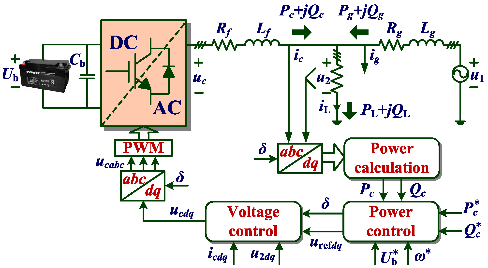
The grid-connected equivalent model of the inverter is illustrated in Figure 2, which consists of the battery pack, the GFM inverter, the L filter, the feeder impedance, and loads. The voltage source $u_1$ is used to simulate the distribution network, and $L_f$ and $R_f$ are the filter inductance and parasitic resistance. The GFM inverter is connected with the distribution network in parallel with the load.

Applying Kirchhoff’s laws, the mathematical model of the GFM inverter is established as

$$L_f{\displaystyle \frac{d{i}_c}{dt}}+R_f{i}_c=u_c-u_2,$$

(4)

where $u_c$ represents the output voltage of the GFM inverter, and $i_c$ represents the compensation current.

According to (4), using the $dq$ rotating coordinate transformation, the dynamic equations of the GFM inverter can be rewritten as

$$\left\{\begin{array}{c}{L}_f{\dot{i}}_{cd}+R_f{i}_{cd}-\omega L_f{i}_{cq}=u_{cd}-u_{2d},\hfill \\ L_f{\dot{i}}_{cq}+R_f{i}_{cq}+\omega L_f{i}_{cd}=u_{cq}-u_{2q},\hfill \end{array}\right.$$

(5)

where $i_{cd}$, $i_{cq}$, $u_{cd}$, $u_{cq}$, $u_{2d}$, and $u_{2q}$ denote $dq$-axis components of $i_c$, $u_c$, and $u_2$, respectively.

The following two aspects need to be analyzed and achieved. On the one hand, the power required by the load should be shared by the grid and the GFM inverter to reduce the transmission loss of the electric energy on the feeder. There exists $▵Q_c>0$ such that $Q_{\mathrm{L}}=Q_g+▵Q_c$ holds. On the other hand, consider whether the positions of distribution transformer taps can satisfy the voltage demand. Take a limited number of tap-changer operations so that the load voltage reaches the national standard of P.R. China (GB/T 12325-2008: −10%∼7%).

3. Main Results

To achieve synchronization between the GFM inverter and the distribution network, a modified robust power control is devised, whose control block diagram is depicted in Figure 3. The integrator is employed in the P-f branch to achieve rapid phase angle synchronization and eliminate the static error [21]. A voltage feedforward is incorporated in the Q-U branch to reduce the voltage sag. Moreover, an integrator is attached to the Q-U branch to ensure no static error of the voltage. The modified power control laws are expressed as

$$\begin{array}{c}{U}_{\mathrm{ref}}={\displaystyle \frac{K_Q}{s}}((U^{*}-U_2)(k_{\mathrm{p}V}+{\displaystyle \frac{k_{\mathrm{i}V}}{s}})-m_Q(Q_c-Q_c^{*})),\hfill \end{array}$$

(6)

$$\begin{array}{c}\delta ={\displaystyle \frac{K_P}{s}}(w^{*}-m_P(P_c-P_c^{*})),\hfill \end{array}$$

(7)

where ${\displaystyle \frac{w_c}{s+w_c}}$ with the cut-off frequency $w_c$ represents the low-pass filter, $U_{\mathrm{ref}}$ and $U^{*}$ denote the reference amplitude of the voltage control input and the rated voltage, respectively, $U_2$ denotes the terminal voltage amplitude, $K_Q$ and $K_P$ denote the integrator gains, $k_{\mathrm{p}V}$ and $k_{\mathrm{i}V}$ denote the proportional and integral gains of the PI controller, $m_Q$ and $m_P$ denote the droop coefficients, $Q_c$, $P_c$, $Q_c^{*}$, and $P_c^{*}$ are the output active power and reactive power and corresponding references, and $w^{*}$ is the fundamental angular frequency reference. The active/reactive power loops use negative feedback to enforce droop behavior (reducing frequency/voltage when output power exceeds the reference). In contrast, the frequency/voltage reference adjustments utilize positive feedback to ensure the inverter increases power injection during grid disturbances (e.g., frequency dips or voltage sags), thereby emulating the dynamics of a synchronous generator.

To extract the fundamental frequency component and attenuate high-frequency switching noise from the measured output power, a first-order low-pass filter (LPF) is applied, yielding the filtered power signals $P_c$ and $Q_c$ used in the power control loops. Inverter output power measurements inherently contain significant high-frequency ripple components due to pulse width modulation. Feeding this noisy signal directly into the power control loop would cause undesirable oscillations in the inverter’s output voltage magnitude and frequency references ($U_{ref}$, ${\omega }_{ref}$), degrading performance and potentially destabilizing the system. The continuous-time transfer function of the LPF is $G_{LPF}\left(s\right)=1/(1+s\ast T_f)$ [34]. It is related to the time constant by $f_{cutoff}=1/(2\pi \ast T_f)$ Hz. Typical values for grid-forming inertia emulation range from 1 Hz to 10 Hz.

The voltage feedforward control diagram is depicted in Figure 4. Applying voltage amplitude control instead of voltage vector control facilitates reducing the complexity of input reference deviation control. The voltage control input $U_{\mathrm{ref}}$ follows its reference $U_2^{*}$ via a PI controller to ensure static error-free tracking. It follows from Figure 4 that the synchronous frequency deviation and the system output voltage deviation are fed to the compensation current reference $i_{cdq}^{*}$.

To control the inverter voltage more precisely, the terminal voltage reference $u_{2dq}^{*}$ is fed forward to the modulation voltage input, as illustrated in Figure 5. The current control law can be derived as

$$\left\{\begin{array}{c}{u}_{2d}={\gamma }_{\mathrm{p}}(i_{cd}^{*}-i_{cd})+R_f{i}_{cd}-w{L}_f{i}_{cq}+u_{2d}^{*},\hfill \\ u_{2q}={\gamma }_{\mathrm{p}}(i_{cq}^{*}-i_{cq})+R_f{i}_{cq}+w{L}_f{i}_{cd}+u_{2q}^{*},\hfill \end{array}\right.$$

(8)

where ${\gamma }_{\mathrm{p}}$ represents the proportional gain.

Considering the filtering loss, we have

$$\left\{\begin{array}{c}{i}_{cd}^{*}=i_{cd}-(u_{2d}^{*}-u_{2d})/{\gamma }_{\mathrm{p}}+w{L}_f(i_{cd}+i_{cq})/{\gamma }_{\mathrm{p}},\hfill \\ i_{cq}^{*}=i_{cq}-(u_{2q}^{*}-u_{2q})/{\gamma }_{\mathrm{p}}+w{L}_f(i_{cq}+i_{cd})/{\gamma }_{\mathrm{p}}.\hfill \end{array}\right.$$

(9)

According to (9), the original voltage feedback is replaced by the current feedback to improve the current response. The current controller with the current gain ${\mathcal{G}}_i\left(s\right)$ is expressed as

$$i_{cdq}^{*}={\mathcal{G}}_i\left(s\right)i_{cdq}+{\mathcal{G}}_i\left(s\right)w{L}_f(i_{cd}\pm i_{cq})/{\gamma }_{\mathrm{p}}.$$

(10)

Substituting (10) into (9) yields

$$\left\{\begin{array}{c}{i}_{cd}^{*}={\displaystyle \frac{{\mathcal{G}}_i\left(s\right)(u_{2d}^{*}-u_{2d})}{(1-{\mathcal{G}}_i\left(s\right)){\gamma }_{\mathrm{p}}}},\hfill \\ i_{cq}^{*}={\displaystyle \frac{{\mathcal{G}}_i\left(s\right)(u_{2q}^{*}-u_{2q})}{(1-{\mathcal{G}}_i\left(s\right)){\gamma }_{\mathrm{p}}}}.\hfill \end{array}\right.$$

(11)

Since the quasi-proportional resonance controller can well achieve static error-free tracking of AC signals, ${\mathcal{G}}_i\left(s\right)$ can be derived as

$${\mathcal{G}}_i\left(s\right)={\displaystyle \frac{k_{\mathrm{pr}}{\gamma }_{\mathrm{p}}{s}^2+2{\gamma }_{\mathrm{p}}{w}_c(k_{\mathrm{pr}}+k_{\mathrm{r}})s+k_{\mathrm{pr}}{\gamma }_{\mathrm{p}}{w}_{\mathrm{r}}^2}{\mathcal{A}{s}^2+\mathcal{B}s+\mathcal{C}}},$$

(12)

where $\mathcal{A}={\gamma }_{\mathrm{p}}{k}_{\mathrm{pr}}+1$, $\mathcal{B}=2{\gamma }_{\mathrm{p}}{k}_{\mathrm{pr}}{w}_c+2{\gamma }_{\mathrm{p}}{k}_{\mathrm{r}}{w}_c+2w_c$, $\mathcal{C}=({\gamma }_{\mathrm{p}}{k}_{\mathrm{pr}}+1)w_{\mathrm{r}}^2$, $k_{\mathrm{pr}}$, and $k_{\mathrm{r}}$ are proportional and resonant gains, respectively, and $w_{\mathrm{r}}$ is the resonant bandwidth.

The current control framework is illustrated in Figure 5. It can be seen from (12) that the current control with the gain ${\mathcal{G}}_i\left(s\right)$ achieves the same function as the original voltage loop control. The current controller instead of the terminal voltage feedback simplifies the control framework and improves the current control accuracy.

The power synchronization and the current control of the GFM inverter ensure the terminal voltage stability of the distribution network and achieve reactive power compensation. When the terminal voltage exceeds the limit, the proposed GFM scheme is activated to provide users with partial active support and reactive power compensation, alleviating voltage fluctuation and reducing the power supply pressure of the distribution network. The schematic of the proposed GFM scheme is presented in Figure 6, where $G_{cc}\left(s\right)={\gamma }_{\mathrm{p}}{\mathcal{G}}_i\left(s\right)(1+w{L}_f/{\gamma }_{\mathrm{p}})-{\gamma }_{\mathrm{p}}$, and the specific expression is as follows:

$$G_{cc}\left(s\right)={\displaystyle \frac{\mathfrak{C}{s}^2+\mathfrak{D}s+\mathfrak{E}}{\mathcal{A}{s}^2+\mathcal{B}s+\mathcal{C}}},$$

(13)

where $\mathfrak{C}=2k_{\mathrm{pr}}{\gamma }_{\mathrm{p}}^2+k_{\mathrm{pr}}{\gamma }_{\mathrm{p}}w{L}_f+{\gamma }_{\mathrm{p}}$, $\mathfrak{D}=4k_{\mathrm{pr}}{\gamma }_{\mathrm{p}}^2{w}_c+4{\gamma }_{\mathrm{p}}^2{k}_{\mathrm{r}}{w}_c+2k_{\mathrm{pr}}{\gamma }_{\mathrm{p}}{w}_{c}w{L}_f+2k_{\mathrm{r}}{\gamma }_{\mathrm{p}}{w}_{c}w{L}_f+2{\gamma }_{\mathrm{p}}{w}_c$, $\mathfrak{E}=2k_{\mathrm{pr}}{\gamma }_{\mathrm{p}}^2{w}_{\mathrm{r}}^2+k_{\mathrm{pr}}{\gamma }_{\mathrm{p}}{w}_{\mathrm{r}}^{2}w{L}_f+{\gamma }_{\mathrm{p}}{w}_{\mathrm{r}}^2$.

In addition, by regulating the distribution transformer tap changers, the transformation ratio $k_1$ of the transformer may be altered to improve the terminal voltage quality at the source of the line. In what follows, we construct a multi-objective optimization model with the maximum qualified rate of the load voltage and the minimum switching times of the distribution transformer tap changers and use the weighted method to simplify the processing. The objective function is defined as

$$\begin{array}{c}\hfill \left\{\begin{array}{c}{\Pi }_1=min\left\{S(\beta ,{\Xi }_i)\right\},\hfill \\ {\Pi }_2=min\left\{M(\alpha ,{\Gamma }_j)\right\},\hfill \\ 198V\le u_2\le 235.4V,\hfill \\ Q_{\mathrm{L}}-\Delta Q\le Q_g\le Q_{max},\hfill \\ k_{1imin}\le k_{1i}\le k_{1imax}.\hfill \end{array}\right.\end{array}$$

(14)

For the $\alpha$ load nodes of the distribution network, the terminal voltage before optimization is defined as

$$u_2=[u_{21},u_{22},\dots ,u_{2(\beta -1)},u_{2\beta }].$$

(15)

The terminal voltage after voltage regulation is obtained as

$${\tilde{u}}_2=[{\tilde{u}}_{21},{\tilde{u}}_{22},\dots ,{\tilde{u}}_{2(\beta -1)},{\tilde{u}}_{2\beta }].$$

(16)

According to the national standard, the allowable voltage fluctuation range of 220 V side is −7%∼10%. When the voltage exceeding limit occurs, the terminal voltage will exceed the allowable upper voltage limit ${\overline{u}}^{*}$ and lower voltage limit ${\underline{u}}^{*}$. The matrix $\Xi$ is determined as $\Xi =[{\Xi }_1,{\Xi }_2,\dots ,{\Xi }_{(\beta -1)},{\Xi }_{\beta }]$. When ${\tilde{u}}_2\in [{\underline{u}}^{*},{\overline{u}}^{*}]$, ${\Xi }_{\beta }=0$ and ${\Xi }_{\beta }=1$ otherwise.

The qualified results of the terminal voltage are obtained as

$$S=\sum _{i=1}^{\beta }{\Xi }_i.$$

(17)

There are five transformation ratios for substation distribution transformers, including 10.5/0.4, 10.25/0.4, 10/0.4, 9.75/0.4, and 9.5/0.4. When reactive power compensation and voltage regulation cannot satisfy the voltage standard, the on-load voltage regulation is necessary for distribution transformers. The following are the key circumstances that require transformer tap adjustment: (1) Large sustained load increases or generation drops cause voltage to exceed the inverter’s reactive power capability. (2) Faults or abrupt grid disconnections cause deep voltage sags/swells that inverters cannot correct instantaneously. (3) Feeders with limited GFM inverter penetration or high impedance (weak grid) lack sufficient distributed reactive power resources. (4) High-distributed generation export raises voltages beyond inverter Q absorption limits. (5) Legacy voltage regulators interact poorly with GFM inverters, creating conflicts. For $\alpha$ low-voltage distribution networks, the distribution transformer tap before optimization is defined as

$$\Psi =[{\Psi }_1,{\Psi }_2,\dots ,{\Psi }_{(\alpha -1)},{\Psi }_{\alpha }].$$

(18)

The distribution transformer tap after voltage regulation is given as

$$\tilde{\Psi }=[{\tilde{\Psi }}_1,{\tilde{\Psi }}_2,\dots ,{\tilde{\Psi }}_{(\alpha -1)},{\tilde{\Psi }}_{\alpha }].$$

(19)

The matrix $\Gamma$ is determined as $\Gamma =[{\Gamma }_1,{\Gamma }_2,\dots ,{\Gamma }_{(\beta -1)},{\Gamma }_{\beta }]$. When $\tilde{\Psi }=\Psi$, ${\Gamma }_{\alpha }=0$ and ${\Gamma }_{\alpha }=1$ otherwise.

The variations in the switching times of the transformer tap changers can be expressed as

$$M=\sum _{j=1}^{\alpha }{\Gamma }_j.$$

(20)

By performing normalization calculation, we have

$$\overline{\Pi }=min({\gamma }_1{\displaystyle \frac{{\Pi }_1-{\Pi }_1^{min}}{{\Pi }_1^{max}-{\Pi }_1^{min}}}+{\gamma }_2{\displaystyle \frac{{\Pi }_2-{\Pi }_2^{min}}{{\Pi }_2^{max}-{\Pi }_2^{min}}}),$$

(21)

where ${\gamma }_1$ and ${\gamma }_2$ are weight coefficients. By numerous experiments, ${\gamma }_1=0.65$ and ${\gamma }_2=0.35$ are selected.

To obtain the optimal solution of the objective function, various types of algorithms for solution are developed, where the meta-heuristic intelligent algorithm has become a emerging solution tool [35]. Thus, this paper presents an EWOA to select the optimal transformer tap configuration scheme. WOA simulates the hunting behavior of humpback whales. Humpback whales mainly have three hunting behaviors, including hunting prey, surrounding prey, and attacking to eat [36].

By identifying the position of prey and individual and using spiral motion, humpback whales gradually surround and approach the prey (optimal solution) to realize position updating [36]. Three social behaviors of humpback whales are described as

$$\left\{\begin{array}{c}{\chi }_{z+1}={\chi }_z^{rand}-\mathsf{\ell }(2\rho -1)|2\rho {\chi }_z^{rand}-{\chi }_z|,\mathrm{Searching},\hfill \\ {\chi }_{z+1}={\chi }_z^{*}-\mathsf{\ell }(2\rho -1)|2\rho {\chi }_z^{*}-{\chi }_z|,\mathrm{Surrounding},\hfill \\ {\chi }_{z+1}={\chi }_z^{*}+|{\chi }_z^{*}-{\chi }_z|e^{\sigma \nu }cos\left(2\pi \nu \right),\mathrm{Attacking},\hfill \end{array}\right.$$

(22)

where z is the current iteration number, ${\chi }_{z+1}$ and ${\chi }_z$ denote the position of the next iteration updating and the current position, respectively, ${\chi }_z^{rand}$ and ${\chi }_z^{*}$ denote the random position of the whale individual and the current optimal position, respectively, $\rho \in [0,1]$, $\nu \in [-1,1]$, $\sigma$ is the spiral motion constant, ℓ is the attenuation factor, which decreases linearly from 2 to 0 with the iteration, and $\mathsf{\ell }(2\rho -1)\in [-2,2]$.

In the process of attacking and eating, humpback whales shrink their encirclement while swimming in a spiral. To simulate this predation process, the probability $\lambda \in (0,1)$ is introduced to determine the position updated mode. In this paper, $\lambda =0.5$ is chosen.

The boundaries of hunting prey and surrounding prey can be set forcibly since the position of each individual is random and unknown. Set $\mathsf{\ell }(2\rho -1)\in [-1,1]$. When $\mathsf{\ell }(2\rho -1)>1$ or $\mathsf{\ell }(2\rho -1)<-1$, humpback whales are forced to search for prey to implement the position updating.

The randomness and dispersion of the initial position of the individual may affect the convergence process of the algorithm. To accelerate the convergence rate and improve the search accuracy of the algorithm, an adaptive attenuation factor ${\mathsf{\ell }}^{\eta }$ is proposed, which changes from linear reduction to adaptive reduction based on the target distance, thereby improving the global search ability of the algorithm. The adaptive attenuation factor is designed as

$${\mathsf{\ell }}^{\eta }=cos({\displaystyle \frac{\pi z^2}{({\chi }_z^{*}-{\chi }_z+2)z_{max}^2}}).$$

(23)

Consequently, when humpback whales search and surround, the updated position becomes

$$\left\{\begin{array}{c}{\chi }_{z+1}={\chi }_z^{rand}-{\mathsf{\ell }}^{\eta }(2\rho -1)|2\rho {\chi }_z^{rand}-{\chi }_z|,\hfill \\ {\chi }_{z+1}={\chi }_z^{*}-{\mathsf{\ell }}^{\eta }(2\rho -1)|2\rho {\chi }_z^{*}-{\chi }_z|.\hfill \end{array}\right.$$

(24)

The updating results gradually converge to the optimal solution with the iteration. Meanwhile, the algorithm becomes more vulnerable to falling into local optimum. To prevent the algorithm from being trapped in local optimum, a position updating mechanism is developed as

$$\left\{\begin{array}{c}{\chi }_{z+1}={\chi }_z^{*}+|{\chi }_z^{*}-{\chi }_z|e^{\sigma \nu }cos\left(2\pi \nu \right),{\overline{\Pi }}_{z+1}\ne {\overline{\Pi }}_z,\hfill \\ {\chi }_{z+1}={\chi }_z^{*}+|{\chi }_z^{*}-{\chi }_z|e^{\sigma \nu }arctan\left(2\pi \nu \right),{\overline{\Pi }}_{z+1}={\overline{\Pi }}_z.\hfill \end{array}\right.$$

(25)

When the algorithm finds the local optimal solution, it changes the position updated mode and continues to search for the globally optimal solution. When the updated position remains constant, the current solution is the globally optimal solution. The globally optimal ${\overline{\Pi }}^{\mathrm{GS}}$ is given as

$${\overline{\Pi }}^{\mathrm{GS}}=\left\{\begin{array}{c}{\overline{\Pi }}_{z+1},{\overline{\Pi }}_{z+1}\ge {\overline{\Pi }}_z,\hfill \\ {\overline{\Pi }}_z,\mathrm{otherwise}.\hfill \end{array}\right.$$

(26)

4. Simulation Results

To examine the validity of the proposed voltage control strategy, the IEEE 33-node system is used as a case study and extended to a multi-distribution station area, as shown in Figure 7. A distribution network simulation model is established using the PSCAD/EMTDC platform. The system comprises thirty-two branches, three distribution stations, and ninety-nine loads, with a reference power set to 100 MVA. The parameters of EWOA are configured as follows: the individual whale population is 20, and the maximum iteration number is 500. The voltage reference is set to 12.66 kV. The details of the GFM inverter parameters are provided in

Table 1. System parameters.

Parameters and Units	Values	Parameters and Units	Values
$U_{\mathrm{b}}$ (V)	400	$U_2^{*}$ (V)	220
$C_{\mathrm{b}}$ ($\mathsf{\mu }$F)	47	$U^{*}$ (V)	311
$P_c^{*}$ (MW)	1.5	$Q_c^{*}$ (MVar)	0.5
$C_f$ ($\mathsf{\mu }$F)	15	$L_f$ (mH)	4.3
$R_f$ ($\Omega$)	0.6	$Z_g$ ($\Omega ·$${\mathrm{km}}^{-1}$)	1.2 + j3.5
$w_c$ (rad·${\mathrm{s}}^{-1}$)	62.8	$w_{\mathrm{r}}$ (rad·${\mathrm{s}}^{-1}$)	3.2
$w^{*}$ (rad·${\mathrm{s}}^{-1}$)	314	${\gamma }_{\mathrm{p}}$	1.5
$m_P$	0.002	$m_Q$	0.005
$k_{\mathrm{pr}}$	0.2	$k_{\mathrm{r}}$	280.8
$k_{\mathrm{p}V}$	0.04	$k_{\mathrm{i}V}$	0.028
$k_{\mathrm{p}U}$	0.5	$k_{\mathrm{i}U}$	25
$k_{\mathrm{p}w}$	0.6	$k_{\mathrm{i}w}$	5.5

.

Table 2. Comparison of simulation results.

Scheme	Low-Voltagex Side Voltage (V)	User-Side Voltage (V)	Voltage Pass Rate %	Line Loss Ratio %	Average Voltage Deviation %
Pre-implementation	180∼230	170∼230	92.5	11.27	−10.72
Post-implementation	210∼235	200∼230	98.4	9.8	−3.43

compares the results before and after the implementation of the proposed scheme. It is clear from Table 2 that the proposed scheme significantly improves the user-side voltage within the distribution station area. Through algorithmic optimization, the transformer tap changers operate only twice, demonstrating that the proposed regulating scheme effectively minimizes switching actions. The voltage compliance rate improves to 98.6%. In addition to voltage improvements, the system’s power factor is enhanced and power losses are reduced with the integration of GFM inverters. The EWOA generally shows faster convergence and better solution stability compared to the standard WOA. In some cases, the EWOA rapidly narrows in on promising regions due to enhanced exploitation mechanisms. The adaptive parameters prevent stagnation, allowing further improvement in later iterations. Despite the enhancements, the EWOA is not immune to convergence issues under certain conditions. Under highly deceptive or rugged scenes, the algorithm may become trapped in local optima. As dimensionality increases significantly (e.g., >100), the convergence speed drops, and the likelihood of premature convergence increases unless dimensionality reduction or feature selection is applied. Moreover, if the initial population is too clustered or lacks coverage, the EWOA may converge to suboptimal regions early. To mitigate these aspects, we recommend hybridizing the EWOA with local search refinements (e.g., gradient-based techniques or Lévy flight mechanisms) in future research. The compared results using the conventional droop, the adaptive virtual synchronous generator (VSG), the PI with fuzzy tuning, and the proposed strategy with the WOA and EWOA are listed in

Table 3. Performance comparison with different strategies.

Strategy	Conventional Droop	Adaptive VSG [23]	PI with Fuzzy Tuning [12]	Proposed Strategy
Optimization method	None	Particle Swarm Optimization	Genetic Algorithm	WOA	EWOA
Iterations	None	149 iterations	156 iterations	98 iterations	56 iterations
Stability	Oscillation	Stable	Oscillation	Stable	Stable
Convergence rate	2.113 s	1.292 s	1.897 s	873 ms	480 ms
Robustness	Weak	Moderate	Limited	Strong	Strong
Voltage qualification rate	92.5%	97.1%	96.3%	98.2%	98.4%
Steady-state error	2.1%	0.52%	0.86%	0.49%	0.41%
Remarks	Simple implementation	Dynamic inertia adaptation	Lacks adaptability	Robustness and slow response speed	Better convergence and robustness

.

The system dynamic results before and after implementing the proposed approach are displayed in Figure 8. As illustrated in Figure 8a when the proposed approach is not activated, the load voltage reaches only 188 V, which is seriously below the national allowable lower voltage limit. This condition undermines voltage stability and impedes the safe and efficient operation of the distribution network. Upon activating the proposed scheme, the load voltage apparently improves, which reaches the voltage reference at the terminal of the distribution station area. At approximately $t\approx 4$ seconds in Figure 8b, when the proposed control method is activated, a transient voltage rise is observed in Phase B. This behavior is consistent with the controller initiating a corrective action to mitigate an imbalance or disturbance. This peak value remains within the tolerable range specified by the protection limits of the system’s components. The overcurrent event is very short-lived, lasting less than $\Delta \approx 100$ ms, and does not trigger instability in the system. This transient effect is a controlled trade-off to achieve fast convergence and improved steady-state performance and does not compromise the long-term voltage quality goals of the proposed strategy. The three-phase output voltage and power of the GFM inverter are shown in Figure 8b–d. The reactive power compensation provided by the GFM inverter reduces the reactive power flow from the grid, thereby lowering the line transmission losses and enhancing the overall power quality of the distribution network. The results confirm that the proposed regulation method is effective and feasible.

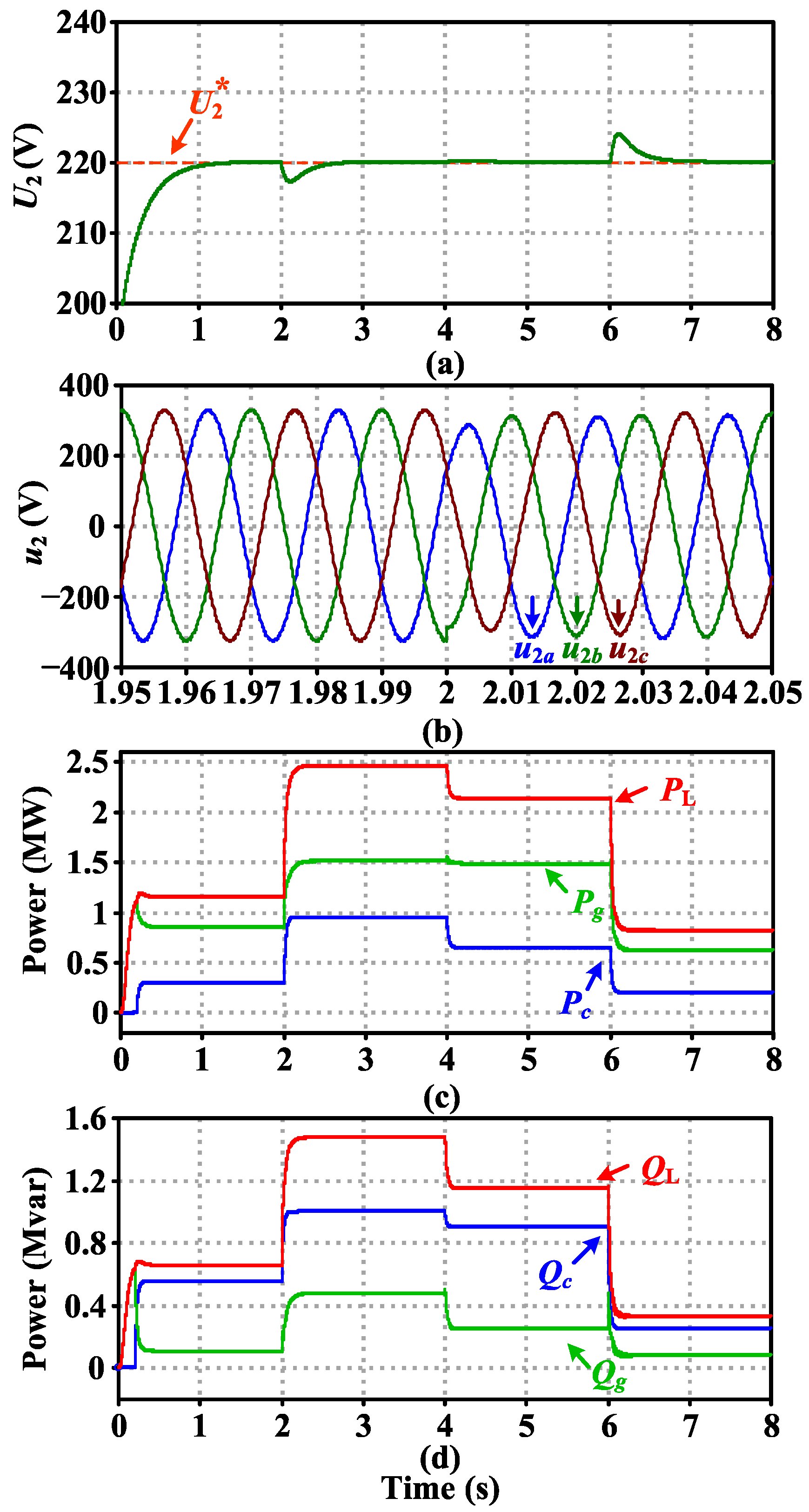
The system dynamic results with load variations are illustrated in Figure 9. The load variations simulate changes in user electricity consumption. The power increases and decreases represent the surges and sags in user demand, respectively. It can be observed from Figure 9a,b that, when the power consumption changes, the proposed method rapidly stabilizes the terminal voltage, effectively reducing voltage fluctuations and improving user voltage quality. Moreover, the proposed approach demonstrates a satisfactory power compensation effect, further improving the power quality of the distribution network, as shown in Figure 9c,d.

To validate the plug-and-play performance of the proposed control strategy, a test for GFM inverters is conducted. The dynamic results of the plug-and-play performance are depicted in Figure 10. During the initial operation, only one inverter is connected to the system. In Figure 10a, the terminal output voltage can precisely reach the voltage reference 220 V, achieving effective voltage compensation. At $t=2$ s, two inverters are inserted into the system. The output power of the inverter increases, which reduces the output of the power grid and decreases the power transmission loss. At $t=4$ s, one inverter is disconnected from the system. The other two inverters continue to provide power compensation for the system. The dynamic waveforms of the active power and reactive power of the GFM inverter are exhibited in Figure 10c,d. It can be observed from Figure 10e that the d-axis component of the inverter voltage has satisfactory dynamic and steady-state effects.

Figure 11 shows the dynamic results of the GFM inverter reverse charging, in which the terminal output voltage, power, and d-axis component of $u_c$ are presented in Figure 11a–e. When the power consumption of users is in the valley, it is necessary to charge the battery system that supplies power to the inverter with excess electricity. In the first 4s, we simulated to charge one inverter. At $t=4$ s, the load power remains unchanged, and the power grid supplements the power for two inverters at the same time. It can be seen that the output voltage curves are smooth and have fast dynamic response. Even in the process of the reverse charging, the terminal voltage of the power grid is consistently maintained in an ideal state.

While the proposed robust control strategy has shown promising performance, several challenges remain in real-world implementation. The simulation models are typically developed under ideal conditions—accurate system parameters and ideal sensors and actuators. In reality, system dynamics often involve unmodeled nonlinearities, parameter drift, or time-varying characteristics that are difficult to capture completely. While external disturbances and noise are included in simulations, their real-world nature is often more complex and unpredictable. The simulations do not fully account for hardware limitations such as sensor resolution, actuator saturation, time delays, communication latencies, or processor constraints. These non-idealities can significantly affect control accuracy and stability. Furthermore, situations like sudden system failures, structural damage, or external shocks may not be represented in controlled simulation scenarios.

5. Conclusions

This paper proposed a robust voltage control strategy for GFM inverters in distribution networks to realize power support and voltage governance. At the load terminal, the GFM control approach included three control loops comprising a power synchronization control loop, a voltage feedforward control loop, and a current control loop. The terminal voltage reference was added to the modulation voltage input, which improves the voltage regulation accuracy. The double-loop control was replaced by a current-loop control, simplifying both the controller construction and computational process and improving the current response. Moreover, an EWOA was proposed to attain a globally optimal voltage configuration, which employed the proposed adaptive attenuation factor and position updating mechanism to accelerate convergence and improve optimization precision. The simulation results validated the effectiveness of the proposed approach, demonstrating satisfactory control performance in achieving voltage governance, power compensation, and dynamic response.