Integrated Cascade Control and Gaussian Process Regression–Based Fault Detection for Roll-to-Roll Textile Systems

Abstract

Roll-to-roll (R2R) manufacturing processes demand precise control of web or yarn velocity and tension, alongside robust mechanisms for handling system failures. This paper presents an integrated approach combining high-performance control with reliable fault detection for an experimental R2R system. A model-based cascade control strategy is designed, incorporating system identification, radius compensation for varying roll diameters, and a Kalman filter to mitigate load sensor noise, ensuring accurate regulation of yarn velocity and tension under normal operating conditions. In parallel, a data-driven fault detection layer uses Gaussian Process Regression (GPR) models, trained offline on healthy operating data, to predict yarn tension and motor speeds. During operation, discrepancies between measured and GPR-predicted values that exceed predefined thresholds trigger an immediate shutdown of the system, preventing material loss and equipment damage. Experimental trials demonstrate tension regulation within ±0.02 N and velocity errors below ±5 rad/s across varying roll diameters, while yarn-break and motor-fault scenarios are detected within a single sampling interval (<100 milliseconds) with zero false alarms. This study validates the integrated system’s capability to enhance both the operational precision and resilience of R2R processes against critical failures.

1. Introduction

Roll-to-roll (R2R) systems are widely used in textile manufacturing to transport yarn or fabric between an unwinding roll and a rewinding roll under controlled tension. In such systems, an unwinder motor feeds yarn from a supply roll, a rewinder motor pulls the yarn onto a take-up roll, and a load cell measures the yarn tension. Proper regulation of yarn tension and motor velocity is crucial for product quality—optimal tension yields strong, uniform fabric [1], whereas poor tension control can cause weave defects and yarn breakage, leading to production interruptions and increased costs [2]. Thus, maintaining the desired tension throughout the process is a primary concern in textile R2R operations.

Achieving consistent tension is challenging due to the system’s time-varying dynamics and disturbances. As the winding process progresses, the radii of the unwinder and rewinder rolls change continuously, which alters the relationship between motor speed and linear yarn velocity [3,4,5]. For example, if the unwinder’s roll diameter decreases, it must rotate faster to supply yarn at the same linear speed, and failing to adjust for this can cause tension fluctuations. Changes in operating speed (throughput) further introduce transient tension swings that must be controlled. Traditionally, mechanical solutions such as adjustable brakes or flywheels were used to mitigate tension variations [4,6,7]. Modern approaches instead employ active control systems: recent work by the authors introduced a model-based cascade control scheme that coordinates yarn tension control (outer loop) with the motor position/velocity control inner loop [8,9]. This cascade control architecture, augmented with feedback and a disturbance observer, proved effective in keeping tension stable under varying roll diameters and speeds [9,10]. Additionally, a Kalman filter-based signal processor was used in that system to reduce load-cell noise and improve measurement reliability [11]. While such robust control strategies can maintain performance during normal conditions, they do not inherently detect or handle fault conditions such as yarn breakage or motor failures.

Fault detection in textile R2R systems is vital for safety and productivity. A sudden yarn break can drop the tension to zero almost instantaneously, causing a loss of fabric tension and potentially allowing the motors to spin freely or entangle the yarn [12] If not detected promptly, a yarn breakage incident can damage equipment and material, as well as cause downtime for cleaning and re-threading the machine [13,14]. Similarly, a loss of power or torque in one of the motors (unwinder or rewinder) constitutes a serious fault—it may lead to either slack (if the rewinder fails and unwinder keeps feeding) or excessive tension (if the unwinder fails and the rewinder continues pulling) [12,15]. In both scenarios, the cascade controller alone would attempt to compensate for the unexpected change (e.g., the tension controller might drive the rewinder motor harder to regain tension on a broken yarn), which could exacerbate the situation. Therefore, an automated fault detection mechanism is needed to immediately recognize faults such as yarn breakage or motor drive failure and take protective action (such as halting or disengaging the motors) before significant damage occurs. However, detecting these faults in real time is non-trivial because the system’s sensor signals naturally exhibit noise and variability. For instance, the tension sensor readings fluctuate due to machine vibration and measurement noise, and the normal tension level itself varies with roll radius and setpoint changes. These factors make it difficult to distinguish a genuine fault from benign disturbances using simple threshold-based logic [16,17].

Recent advances in data-driven diagnostics and maintenance planning further illustrate the diversity of modern fault-management strategies. For example, a multi-scale prototype fusion network has been shown to fuse hierarchical feature maps and achieve state-of-the-art surface anomaly detection and precise localization in industrial settings [18]. An intelligent diagnosis method based on residual-signal analysis has demonstrated rapid, reliable early fault detection in electric-hydraulic control systems, catching incipient failures before they propagate [19]. Furthermore, in the realm of maintenance optimization, an adaptive multi-strategy particle swarm-based framework balances cost, reliability, and downtime under uncertainty, yielding a multi-objective strategy for complex-system upkeep [20].

These studies underscore the trend toward hybrid learning-based and optimization-based architectures and motivate our choice of a probabilistic, GPR-based monitoring layer for continuous-process fault detection—in particular, because conventional, model-based schemes rely on fixed thresholds and cannot distinguish between benign transients (e.g., tension overshoots during rapid speed changes) and genuine faults. By contrast, GPR inherently quantifies uncertainty, enabling the system to learn the full range of normal dynamic behaviors and flag only those deviations that fall outside its credible prediction interval.

To address this challenge, the present work proposes a Gaussian Process Regression (GPR) based fault detection system for the textile R2R tension control setup. GPR is a data-driven modeling approach that uses a Bayesian non-parametric regression framework to learn complex input–output relationships. In the context of our R2R system, we leverage GPR to develop a “virtual sensor” model of the process: using data collected under normal operating conditions, the GPR is trained offline to capture the relationship between the system inputs and the key outputs. This offline-trained model enables sensorless prediction of the system’s behavior in real time—essentially, given the current states and inputs, the GPR model can predict what the system states (yarn tension, motor velocities) should be if the system is functioning normally. The predicted signals are then continuously compared with the actual measured signals from the load cell and motor encoders. Under fault-free conditions, the measured and predicted values should closely agree (within the model’s error bounds). If a fault occurs, it will induce an anomaly in the measurements (e.g., tension dropping to zero or deviating sharply) that is inconsistent with the GPR model’s prediction. By monitoring the prediction error, the system can thus detect faults promptly: a significant divergence between the GPR-predicted tension/velocity and the measured values beyond a certain confidence threshold is flagged as a fault condition.

The choice of GPR for this fault detection task is motivated by several advantages of the method in handling complex, noisy systems. First, GPR can inherently model nonlinear relationships and dynamics without requiring an explicit analytical model [21,22] of the R2R system’s changing inertia or roll radius—these effects are learned from the data. This makes it well-suited to capture the R2R process behavior across the full range of roll diameters and operating conditions. Second, GPR provides probabilistic predictions (with an estimated variance), which is valuable for decision-making under uncertainty. The model not only predicts expected tension values but also quantifies uncertainty due to noise or lack of data; this allows the fault detection scheme to distinguish normal fluctuations from out-of-bound anomalies with greater confidence. Indeed, data-driven process monitoring techniques have become increasingly popular in industry, and GPR has been identified as a particularly promising (if underutilized) approach in recent years. Studies on complex industrial processes have reported that GPR-based monitoring can outperform many conventional fault detection methods in accuracy. Moreover, GPR has been successfully applied in various domains for sensor fault detection and data estimation—for example, researchers have used it to estimate missing sensor data and detect instrument drifts in wastewater treatment plants—underscoring its general applicability for detecting anomalies in dynamic systems. By leveraging GPR in our application, we gain a robust modeling tool that adapts to the R2R system’s characteristics and improves the reliability of fault diagnosis.

The remainder of this paper is organized as follows. Section 2 describes the experimental R2R setup and the cascade control algorithm with online radius compensation and Kalman filtering. Section 3 presents the GPR-based fault detection framework and thresholding logic. Section 4 reports the experimental results, Section 5 discusses the key insights, and Section 6 concludes with future research directions.

2. Roll-to-Roll System Overview and Controller Implementation

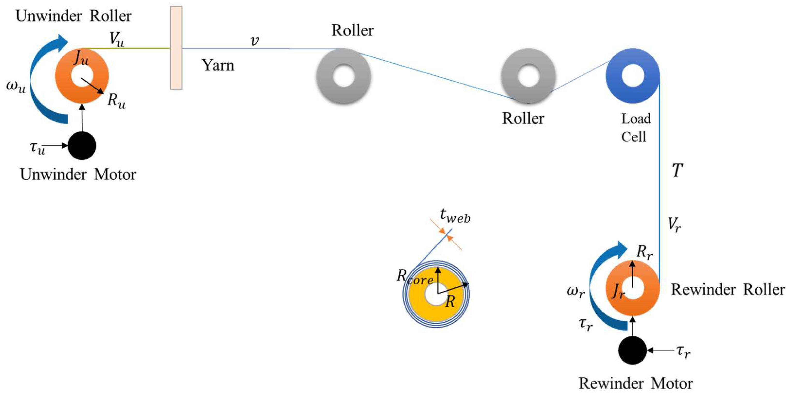
2.1. Experimental Setup

The experimental investigations were carried out using a laboratory-scale roll-to-roll (R2R) system specifically assembled to emulate industrial textile yarn handling operations. The experimental platform (in Figure 1) comprised two servo motors (APMC-FAL01AM8K) rated at 100 W, driving the unwinder and rewinder sections through dedicated L7SA001 motor drivers. The motors operated in torque control mode, aligning effectively with the previously described control framework [23,24].

A precision load cell (M3200 model) with a measurement capacity of up to 50 N was employed to accurately monitor yarn tension. The load cell was positioned strategically on a guide roller located between the unwinder and rewinder sections, ensuring precise measurement of dynamic tension variations during the yarn transport process [9,25].

The core control and data acquisition operations were managed by a QUANSER QPIDe control board, which is a high-precision microcontroller developed by National Instruments. This controller features an analog output range of ±10 V and provides a high-resolution (19-bit) analog-to-digital conversion capability, thereby delivering accurate PWM control signals to the servo motors [23]. MATLAB (2022b software interfaced directly with the QUANSER control board via its external mode function, enabling real-time control algorithm execution and fault detection logic processing [24].

The yarn utilized in the experiments had well-characterized mechanical properties, including stiffness (Young’s modulus) and cross-sectional area, which are critical parameters for effective system modeling and control performance assessment [25,26]. Experimental conditions simulated realistic operational scenarios, transitioning from fully wound to fully unwound states during operation [27]. Detailed specifications of all key hardware components used in the experimental setup are comprehensively listed in

Table 1. Hardware specifications.

Component	Parameter	Value/Description
Unwinder Motor	Type	Servo Motor
	Model No.	APMC-FAL01AM8K
	Max Torque	0.96 Nm
	Encoder Resolution	2500 PPR
	RPM	3000
Rewinder Motor	Type	Servo Motor
	Model No.	APMC-FAL01AM8K
	Max Torque	0.96 Nm
	Encoder Resolution	2500 PPR
	RPM	3000
Load Sensor	Type	Industrial pressure transducer
	Range	0.1–50 N
	Sensitivity	$\pm 0.1N$
	Location	On intermediate guide roller
Data Acquisition	Hardware	National Instrument QUANSER Board
	Sampling Rate	200 kHz
Yarn	Material	Polyester
	Stiffness (E)	Value specific to the identified yarn

.

It is crucial to recognize that the controller’s performance, particularly parameters tuned based on system identification, is inherently linked to the properties of the specific yarn used during these identification experiments. Performance may differ when processing materials with significantly different stiffness or frictional characteristics.

2.2. System Dynamics Modeling

A mathematical model representing the dominant dynamics of the R2R system is essential for model-based controller design. The model [28,29,30] is derived using fundamental physical principles, primarily Newton’s laws for rotation and translation. Key assumptions typically include linear elasticity of the yarn (Hooke’s law), negligible gravitational effects (sagging), and perfect traction between the yarn and the rollers. Figure 2 illustrates the core dynamic model of our roll-to-roll line: the unwinder and rewinder rolls are each represented by their rotational inertias ($J_u, J_r$) and friction coefficients ($B_u, B_r$), driven by motor torques ${\tau }_u, {\tau }_r$. The interconnecting yarn segment transmits tension $T$ between the two axes, and its elasticity is captured by the stiffness constant $k$. The block diagram in Figure 2 highlights how the changing roll radii—and hence inertias—alter the mechanical coupling that the control system must regulate. For a comprehensive list of the symbols used in the mathematical equations and their definitions, please refer to

Table A1. List of symbols and their definition.

Variable	Definition
$J_u$	Moment of inertia of the unwinder roll
$J_r$	Moment of inertia of the rewinder roll
$R_u$	Unwinder radius
$R_r$	Rewinder radius
${\omega }_u$	Angular velocity of unwinder roll
$\dot{{\omega }_u}$	Angular acceleration of unwinder roll
${\omega }_r$	Angular velocity of rewinder roll
$\dot{{\omega }_r}$	Angular acceleration of rewinder roll
$B_u$	Unwinder roll’s rolling friction
$B_r$	Rewinder roll’s rolling friction
$B_{fu}$	Friction torque of unwinder roll
$B_{fr}$	Friction torque of rewinder roll
$T_u$	Yarn tension of unwinder roll
$T_r$	Yarn tension of rewinder roll
${\tau }_u$	Motor torque of unwinder roll (control input)
${\tau }_r$	Motor torque of rewinder roll (control input)
$T$	Yarn tension
$J_{core}$	Inertia of core
${\rho }_m$	Material density
$L$	Roll width
$L_s$	Segment of length
$R$	Radius of roller
$R_{core}$	Core radius of roller
$A$	Yarn cross-sectional area
$E$	Young’s modulus
$v_r$	Linear velocities of rewinder
$v_u$	Linear velocities of unwinder
$k$	Yarn stiffness constant
$T_{ref}$	Desired yarn tension
${\mathrm{C}}_{\mathrm{f}\mathrm{e}\mathrm{e}\mathrm{d}\mathrm{b}\mathrm{a}\mathrm{c}\mathrm{k}}$	Feedback controller
${\mathrm{C}}_{\mathrm{f}\mathrm{e}\mathrm{e}\mathrm{d}\mathrm{f}\mathrm{o}\mathrm{r}\mathrm{w}\mathrm{a}\mathrm{r}\mathrm{d}}$	Feedforward controller
${\omega }_{fb}$	Cutoff frequency of feedback controller
${\omega }_{ff}$	Cutoff frequency of feedforward controller
$K_n$	Control gain
${\tau }_n$	Motor torque
${\mathrm{C}}_{\mathrm{D}\mathrm{O}\mathrm{B}}$	Disturbance observer
${\omega }_{DOB}$	Cutoff frequency of disturbance observer
$Y\left(s\right)$	Output
${\mathsf{\theta }}_{\mathrm{r}\mathrm{e}\mathrm{f}}$	Desired angular position
${\theta }_r$	Measured angle
$T_s$	Tension
${\omega }_{ref}$	Web-speed command
$∆{\theta }_c$	Incremental position command
$J_n$	Nominal inertia
$B_n$	Nominal damping
${\omega }_s$	Angular velocity
v	Yarn linear velocity
ω	Motor angular velocity
$h$	Yarn thickness
$T_k$	Tension variable

.

The rotational dynamics of the unwinder ($u$) and rewinder ($r$) rolls are described by

$$\begin{gathered} J_u\left(R_u\right)\dot{{\omega }_u}={\tau }_u-B_{fu}\left({\omega }_u\right)-T_u{R}_u \\ {J}_r\left(R_r\right)\dot{{\omega }_r}={\tau }_r-B_{fr}\left({\omega }_r\right)-T_r{R}_r \end{gathered}$$

(1)

where J is the moment of inertia (a function of the changing radius $R$), $\omega$ is the angular velocity, $\tau$ is the motor torque (control input, after gear reduction), $B_f$ is the friction torque (often modeled as a combination of viscous and Coulomb friction), and $T$ is the yarn tension at the unwinder ($T_u$) and rewinder ($T_r$) side. The inertia $J\left(R\right)$ changes as $J\left(R\right)=J_{core}+{\rho }_m\pi L(R^2-R_{core}^2)$, where $J_{core}$ is the core inertia, ${\rho }_m$ is the material density, L is the roll width, and $R_{core}$ is the core radius.

The yarn tension dynamics are often modeled based on Hooke’s law, relating tension to the strain in the yarn segment between the rolls. Assuming a dominant tension $T$ in the segment of length $L_s$,

$$\dot{T}={\displaystyle \frac{AE}{L_s}}\left(v_r-v_u\right)={\displaystyle \frac{AE}{L_s}}\left(R_r{\omega }_r-R_u{\omega }_u\right)=k\left(R_r{\omega }_r-R_u{\omega }_u\right)$$

(2)

where $A$ is the yarn cross-sectional area (negligible), E is Young’s modulus, $v_r,\mathrm{a}\mathrm{n}\mathrm{d} v_u$ are the linear velocities at the unwinder and rewinder surfaces, respectively, and k is the stiffness constant.

2.3. System Identification

While the theoretical model structure is physically derived, specific parameters such as friction coefficients, rolling inertia, and effective yarn stiffness (T) require empirical estimation. To accurately estimate the motor-related parameters ($J_u, B_u, J_r, B_r$), we applied Pseudo-Random Binary Sequence (PRBS) inputs and used the Fast Fourier Transform (FFT) on the measured motor and tension signals to compute the Frequency Response Function (FRF), which is the complex ratio of steady-state output to sinusoidal input as a function of the excitation frequency. The measured FRFs for both the unwinder and rewinder axes are overlaid with the theoretical Bode predictions (Figure 3) [23,24].

The yarn stiffness parameter was separately identified by applying a step input with varying positions and analyzing the corresponding tension data obtained from the load cell. This method ensured that the obtained nominal model accurately reflected the system dynamics relevant for subsequent control algorithm design. The nominal model finding process is illustrated in Figure 4 [24].

Validation of the identified parameters involved comparing model predictions to experimental responses using datasets separate from those employed during the identification phase. This validation confirmed the predictive accuracy of the model and ensured the robustness of the designed control algorithms. Identified parameters crucial for the controller design are presented comprehensively in

Table 2. Identified system parameters.

Parameter Symbol	Description	Identified Value	Units
$J_u$	Unwinder roll’s inertia	$7.93{ \times 10}^{-3}$	$\mathrm{K}\mathrm{g}·{\mathrm{m}}^2$
$B_u$	Unwinder roll’s rolling friction	$1.01{ \times 10}^{-2}$
$J_r$	Rewinder roll’s inertia	$4.3367{ \times 10}^{-3}$	$\mathrm{K}\mathrm{g}·{\mathrm{m}}^2$
$B_r$	Rewinder roll’s rolling friction	$1.0292{ \times 10}^{-2}$
$k$	Yarn stiffness constant	$0.8241$	N/m

.

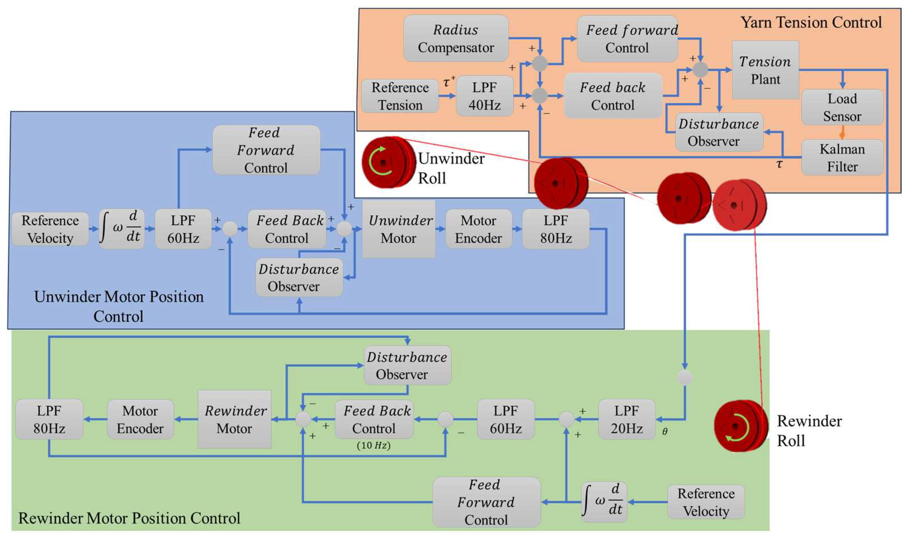
2.4. Cascade Control Algorithm

To achieve simultaneous regulation of yarn tension and web transport in a roll-to-roll (R2R) winding line, we adopt a two-layer cascade control [30,31] scheme (Figure 5). The architecture contains:

• An outer tension loop that converts the desired yarn tension $T_{ref}$ into a position setpoint.
• An inner position loop that drives the rewinder shaft to that setpoint with high bandwidth.

This hierarchy separates the slow, high-inertia yarn mechanics from the fast electromechanical dynamics of the servo motor, yielding good disturbance rejection and simplified tuning [32].

The outer loop converts the desired yarn tension $T_{ref}$ into an incremental position command $∆{\theta }_c$ for the rewinder motor. Three parallel filters—feedback, feedforward, and a disturbance observer (DOB)—are synthesized by pole-zero cancellation on the nominal linear model identified in Section 2.3 as follows:

$$\begin{gathered} {\mathrm{C}}_{\mathrm{f}\mathrm{e}\mathrm{e}\mathrm{d}\mathrm{b}\mathrm{a}\mathrm{c}\mathrm{k}}={\omega }_{fb}\ast K_n\ast {\tau }_n+{\displaystyle \frac{{\omega }_{fb}}{K_n}}.{\displaystyle \frac{1}{s}} \\ {\mathrm{C}}_{\mathrm{f}\mathrm{e}\mathrm{e}\mathrm{d}\mathrm{f}\mathrm{o}\mathrm{r}\mathrm{w}\mathrm{a}\mathrm{r}\mathrm{d}}={\omega }_{ff}\ast K_n\left({\displaystyle \frac{{\tau }_n.s+1}{s+{\omega }_{ff}}}\right) \\ {\mathrm{C}}_{\mathrm{D}\mathrm{O}\mathrm{B}}=Y\left(s\right)\ast {\omega }_{DOB}\ast K_n\left({\displaystyle \frac{{\tau }_n.s+1}{s+{\omega }_{DOB}}}\right)-U\left(s\right)\left({\displaystyle \frac{{\omega }_{DOB}}{s+{\omega }_{DOB}}}\right) \end{gathered}$$

(3)

Here,

• ${\mathrm{C}}_{\mathrm{f}\mathrm{e}\mathrm{e}\mathrm{d}\mathrm{b}\mathrm{a}\mathrm{c}\mathrm{k}}$ = Transfer function of the feedback controller in the outer tension loop.
• ${\omega }_{fb}$ = Cutoff frequency (bandwidth parameter) of the feedback path; governs responsiveness vs. noise rejection (2 Hz in this experiment).
• $K_n$ = Nominal stiffness constant of the selected yarn material.
• ${\tau }_n$ = Time-constant of the first-order low-pass filter used to model the signal delay between the actuator and load cell.
• ${\mathrm{C}}_{\mathrm{f}\mathrm{e}\mathrm{e}\mathrm{d}\mathrm{f}\mathrm{o}\mathrm{r}\mathrm{w}\mathrm{a}\mathrm{r}\mathrm{d}}$ = Transfer function of the feedforward controller in the outer tension loop.
• ${\omega }_{ff}$ = Cutoff frequency (bandwidth parameter) of the feedforward path (40 Hz).
• ${\mathrm{C}}_{\mathrm{D}\mathrm{O}\mathrm{B}}$ = Transfer function of the disturbance observer in the outer tension loop.
• $Y\left(s\right)$ = Laplace-domain representation of the plant output (tension signal) fed into the DOB.
• ${\omega }_{DOB}$ = Cutoff frequency (bandwidth) of the disturbance observer; sets the frequency range for disturbance estimation (1 Hz).
• $U\left(s\right)$ = Laplace-domain representation of the plant input (control signal) used by the DOB reconstruction.

The combined action of these paths keeps the closed-loop tension bandwidth roughly one-tenth of the inner-loop bandwidth, giving a clear separation of timescales and strong disturbance rejection even when yarn elasticity or friction drifts during a roll.

The inner loop drives the rewinder torque $\tau$ so that the measured angle ${\theta }_r$ follows

$${\mathsf{\theta }}_{\mathrm{r}\mathrm{e}\mathrm{f}}\left(k\right)={\mathsf{\theta }}_{\mathrm{r}\mathrm{e}\mathrm{f}}\left(k-1\right)+T_s{\omega }_{ref}\left(k\right)+∆{\theta }_c\left(k\right)$$

(4)

where the first term is the discrete integral of the web-speed command ${\omega }_{ref}$ and the second term is the tension correction from the outer loop. A first-order low-pass filter ahead of the PID suppresses any high-frequency content in $∆{\theta }_c$. With nominal inertia $J_n$ and damping $B_n$, as identified earlier, a pole-placement design yields the feedback compensator,

$${\mathrm{C}}_{\mathrm{f}\mathrm{e}\mathrm{e}\mathrm{d}\mathrm{b}\mathrm{a}\mathrm{c}\mathrm{k}}=\left({\mathrm{J}}_{\mathrm{n}}{s}^2+B_n\right)\ast {\displaystyle \frac{{\omega }_s}{s}}\ast {\displaystyle \frac{{\omega }_{fb}}{s+{\omega }_{fb}}}$$

(5)

which places the position-loop natural frequency at least 10 times higher than that of the outer loop. The unwinder follows the same integrated position trajectory, guaranteeing web-speed consistency, while all fine tension adjustments are affected by the rewinder.

2.4.1. Radius Compensator Design

The changing radii of the unwinder ($R_u$ decreases) and rewinder ($R_r$ increases) significantly affect the system dynamics. Firstly, the moment of inertia ($J_u, J_r$) changes, impacting the rotational dynamics. Secondly, the relationship between motor angular velocity (ω) and yarn linear velocity ($v=R\omega$) changes. A fixed-gain controller tuned for one radius value will perform poorly or become unstable as the radii change.

Radius compensation is therefore necessary. The radii can be estimated online. A common method is to integrate yarn flow,

$$R{\left(t\right)}^2=R{\left(0\right)}^2\pm {\displaystyle \frac{2t_{web}}{\pi L}}\ast N{\int }_0^{t}v\left(\tau \right)d\tau$$

(6)

where $t_{web}$ is the yarn thickness, N number of windings create a layer, L is the width, v(t) is the yarn linear velocity, and the sign depends on whether it is unwinding (−) or rewinding (+). Alternatively, estimates can be derived from motor revolutions and known material thickness. The estimated radii ($R_u\left(t\right),R_r\left(t\right)$) are then used to update the controller gains or parameters within the control algorithm online, effectively adapting the control action to the changing system geometry and inertia. This ensures consistent performance throughout the winding process [8].

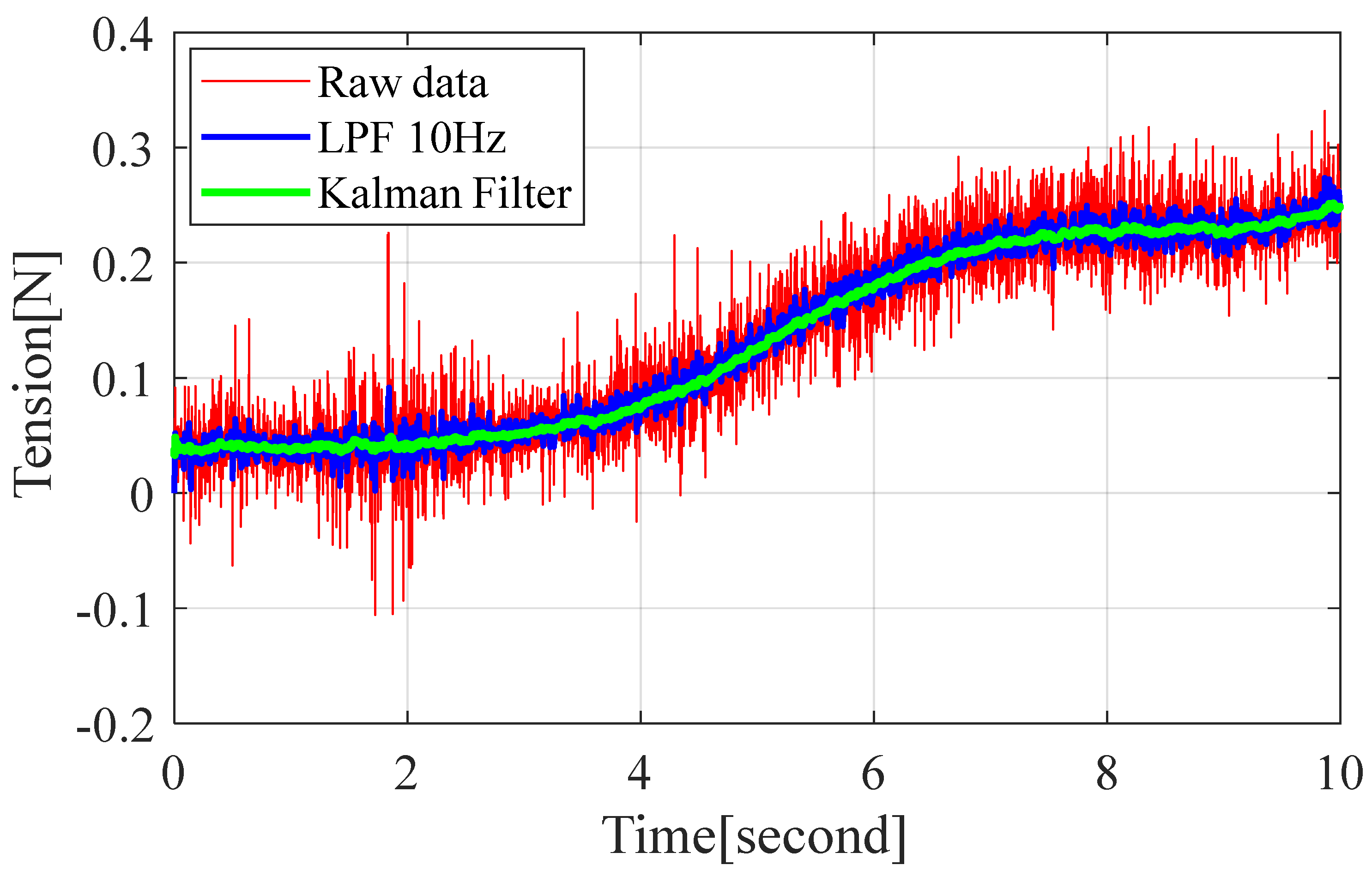
2.4.2. Kalman Filter Design

Load-cell transducers employed for yarn tension monitoring are vulnerable to perturbations generated by mechanical vibration and electromagnetic interference. If these corrupted signals propagate unfiltered through the feedback loop, they can provoke erratic control commands, excite neglected high-frequency dynamics, and erode closed-loop stability. To suppress such effects, a discrete-time Kalman estimator is introduced to furnish an optimal reconstruction of the true tension from noisy measurements.

The observer is formulated on the basis of a reduced-order state–space model that captures the dominant tension dynamics and the associated sensing process. Let the state vector consist solely of the tension variable $T_k$; its temporal evolution is governed by the dynamics presented in Section 2.2, or absent a priori dynamics, by a random-walk process driven by process noise $w_k$. The measurement equation links the load-cell reading $z_k$ to the true tension through additive sensor noise. The complete discrete-time state–space realization, obtained by rearranging (1) and (2), is given by

$$\left\{\begin{array}{c}\dot{x_1}={\displaystyle \frac{EA}{L_s}}\left(R_r{x}_3-R_u{x}_2\right)+{\displaystyle \frac{T_3{R}_u}{L}}{x}_2-{\displaystyle \frac{T_4{R}_r}{L}}{x}_3\\ \dot{x_2}={\displaystyle \frac{R_u}{J_u}}{x}_1-{\displaystyle \frac{B_u}{J_u}}{x}_2+{\displaystyle \frac{{\tau }_u}{J_u}}\\ \dot{x_3}={\displaystyle \frac{R_r}{J_r}}{x}_1-{\displaystyle \frac{B_r}{J_r}}{x}_2+{\displaystyle \frac{{\tau }_r}{J_r}}\end{array}\right.$$

(7)

Once the model parameters and noise covariances are specified, the Kalman recursion yields real-time estimates $T_k$ that are subsequently used by the tension controller, thereby improving the smoothness and robustness of the closed-loop response

$$\begin{gathered} x_{k+1}=F{x}_k+w_k \\ {z}_k=H{x}_k+v_k \end{gathered}$$

(8)

where $x_k$ is the state vector, F is the state transition matrix, H is the measurement matrix, $w_k$ is the process noise (covariance Q), and $v_k$ is the measurement noise (covariance R).

The Kalman filter algorithm proceeds in two steps:

• Prediction: Predict the next state and error covariance based on the model.

$$\begin{gathered} {\widehat{x}}_{k|k-1}=F{\widehat{x}}_{k-1|k-1} \\ {P}_{k|k-1}=F{P}_{k-1|k-1}{F}^T+Q \end{gathered}$$

(9)

2.

Update: Correct the prediction using the current measurement.

$$\begin{gathered} K_k=P_{k|k-1}{H}^T{\left(H{P}_{k|k-1}{H}^T+R\right)}^{-1} \\ {\widehat{x}}_{k|k}={\widehat{x}}_{k|k-1}+K_k(z_k-H{\widehat{x}}_{k|k-1}) \\ {P}_{k|k}=(I-K_{k}H)P_{k|k-1} \end{gathered}$$

(10)

The process- and measurement-noise covariance matrices, $Q$ and $R$, were selected empirically by a systematic trial-and-error procedure until the estimator exhibited an acceptable compromise between measurement-noise attenuation and estimation latency. The resulting state estimate ${\widehat{T}}_k=x_{k|k}$ supplies a markedly smoother feedback signal than that obtained with a conventional low-pass filter, thereby improving closed-loop actuation quality. Figure 6 compares the Kalman-filtered output with a first-order low-pass alternative and highlights the superior noise rejection achieved without sacrificing transient fidelity.

While this filtered estimate is fed to the tension controller, the fault detection algorithm described in Section 4 continues to evaluate residuals against the raw sensor reading; hence, its decision thresholds were adjusted to account for the unfiltered measurement variance [23,24].

3. Fault Detection System Design

3.1. Gaussian Process Regression (GPR) Overview

For fault detection GPR is adopted in this study because, unlike the standard Kalman filter—which presumes a linear Gaussian plant model deliberately tuned for smooth state estimation—GPR provides a non-parametric, probabilistic surrogate that learns the full nonlinear input–output behavior [33] of the healthy process directly from the data; any statistically significant divergence between the GPR one-step-ahead prediction and the real-time measurement therefore exposes incipient faults that the Kalman filter would otherwise attenuate. Although an Extended Kalman Filter (EKF) can, in principle, accommodate nonlinear dynamics, it still relies on an explicit first-principles model and repeated Jacobian linearization, making its accuracy and stability highly sensitive to parameter drifts, unmodelled yarn–web interactions, and aging effects that are inherent in roll-to-roll machinery [34]. By dispensing these modeling assumptions and furnishing a calibrated predictive variance at each operating point, GPR delivers a more robust and statistically rigorous residual for early fault detection across the entire tension-velocity envelope of the plant.

GPR is a non-parametric, Bayesian methodology employed for regression tasks. Unlike parametric models that assume a specific functional form with a fixed number of parameters, GPR defines a probability distribution directly over the space of possible functions that could explain the observed data. This approach provides significant flexibility in modeling complex, potentially nonlinear relationships inherent in datasets [35].

Formally, GPR models [22] the relationship between input features $X=\{x_1, x_2,\dots ,x_N\}$ and corresponding output variables $y=\{y_1, y_2, \dots , y_N\}$ by assuming that the observed outputs y are generated from an underlying latent function $f\left(x\right)$ corrupted by additive noise, typically assumed to be independent and identically distributed Gaussian noise, $ϵ~\mathcal{N}\left(0,{\sigma }_n^2\right):$

$$y=f\left(x\right)+ϵ$$

(11)

The core assumption of GPR is that the latent function $f\left(x\right)$ itself is drawn from a Gaussian Process (GP). A GP is a stochastic process where any finite collection of random variables (in this case, the function values $f\left(x_1\right), \dots , f\left(x_N\right)$ at specific input points) has multivariate Gaussian distribution.

A Gaussian Process is fully specified by its mean function $m\left(x\right)$ and its covariance function, often referred to as the kernel, $k\left(x,x^{\prime }\right):$

$$f\left(x\right)=\mathcal{G}\mathcal{P}\left(m\left(x\right),k\left(x,x^{\prime }\right)\right)$$

(12)

The mean function $m\left(x\right)=E\left[f\right(x\left)\right]$ represents the expected value of the function at input x. For analytical convenience, particularly after normalizing the data, the prior mean function is often assumed to be zero, $m\left(x\right)=0$. The covariance function $k(x,x^{\prime })=E\left[\right(f\left(x\right)-m\left(x\right)\left)\right(f\left(x^{\prime }\right)-m\left(x^{\prime }\right)\left)\right]$ defines the covariance between the function values at two different input points, $x$ and $x^{\prime }$. The kernel function encodes prior beliefs about the properties of the function being modeled, such as its smoothness, length scale, and periodicity. It effectively measures the similarity or correlation between outputs based on their corresponding inputs.

In this study a commonly employed kernel function, the Radial Basis Function (RBF) kernel, also known as the squared exponential kernel, was used:

$$k_{RBF}\left(x,x^{\prime }\right)={{\sigma }_f^2\mathit{exp}\left({\displaystyle \frac{1}{2l^2}}\left|X-X^{\prime }\right|\right)}^2$$

(13)

In this formulation, ${\sigma }_f^2$ represents the signal variance, controlling the overall vertical scale of the function’s variation, and $l$ is the characteristic length-scale parameter, which determines how quickly the correlation between function values decays as the distance between their corresponding inputs increases. The parameters ${\sigma }_f^2$ and $l$, and the noise variance ${\sigma }_n^2$, are hyperparameters of the GPR model, and are typically learned by maximizing the marginal likelihood of the training data.

Given a set of $N$ training observations $D=\left\{\right(X,y\left)\right\}$, GPR utilizes the Bayesian framework to derive the predictive distribution for the output $y^{\ast }$ at a new, unseen input point $x^{\ast }$. (This Bayesian, non-parametric formulation grants two key advantages: (1) it captures arbitrarily complex, nonlinear system behavior without explicit model structure, and (2) it provides an explicit uncertainty estimate ${\sigma }^2$ that we leverage for adaptive, confidence-based fault thresholds.) Based on the GP prior, the joint distribution of the observed training outputs $y$ and the test output $f^{\ast }$ (the latent function value at $x^{\ast }$) is Gaussian as follows:

$$\left(\begin{array}{c}y\\ f\left(x^{\ast }\right)\end{array}\right)=\mathcal{N}(0,\left[\begin{array}{cc}K\left(X,X\right)+{\sigma }^{2}I& K\left(X,X^{\ast }\right)\\ K\left(x^{\ast },X\right)& K\left(x^{\ast },x^{\ast }\right)\end{array}\right])$$

(14)

where $K(X,X)$ is the $N\times N$ covariance matrix evaluated at all pairs of training inputs, $K(X,x^{\ast })$ is the $N\times 1$ vector of covariances between each training input and the test input $K\left(x^{\ast }X\right)=K{\left(X, x^{\ast }\right)}^T,$ and $K\left(x^{\ast },x^{\ast }\right)$ is the prior variance at the test input.

By conditioning this joint distribution on the training data, the resulting posterior predictive distribution for the target output $y^{\ast }$ (including noise) is also Gaussian:

$$p\left(y^{\ast }|x^{\ast }, X, y\right)=\mathcal{N}\left(y^{\ast }\right|{\mu }^{\ast }, {{\sigma }^{\ast }}^2)$$

(15)

The predictive mean ${\mu }^{\ast }$ provides the point estimate for the output at $x^{\ast }$, representing the most likely value based on the model and data. The predictive variance ${{\sigma }^{\ast }}^2$ quantifies the uncertainty associated with this prediction [36]. This inherent ability to provide uncertainty estimates, alongside its capacity to capture complex functional relationships directly from data without restrictive parametric assumptions, makes GPR a powerful tool for regression problems in various scientific and engineering domains [35,36].

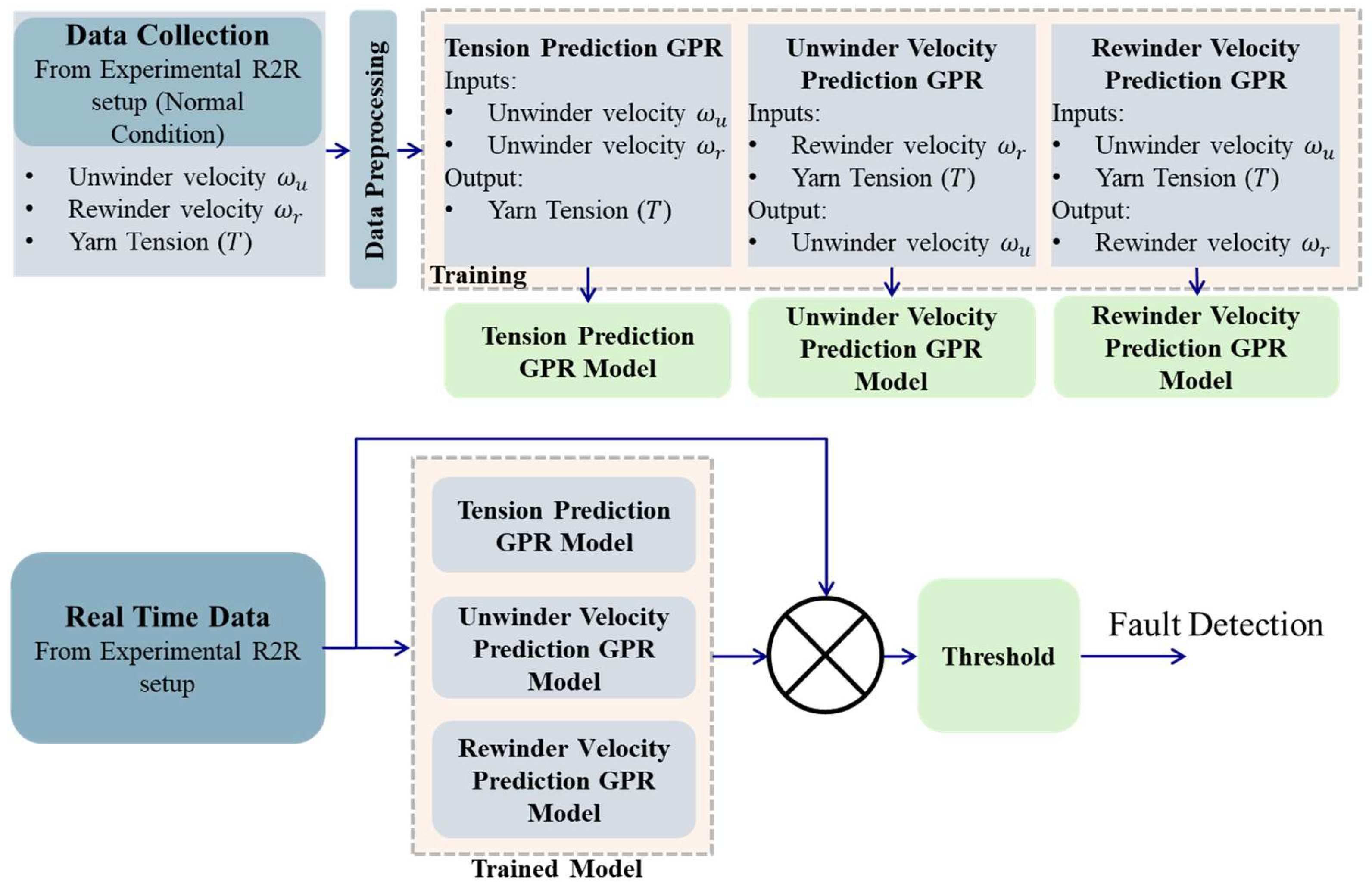
3.2. Offline Data Collection and GPR Training

The GPR models are trained using data collected offline from the experimental R2R setup operating under normal (fault-free) conditions. The data collection process must cover the expected operational range of the system, including various yarn velocity setpoints, tension setpoints, and potentially different stages of roll winding (varying radii), to ensure the GPR models learn the system’s behavior across its intended operating envelope. Data (unwinder velocity, rewinder velocity, yarn tension) is logged at a consistent sampling rate for a sufficient duration. In our study, 30 data-collection sessions were performed under fault-free operation. Each session lasted 30 s at a 1 ms sampling interval (1 kHz), yielding 30,000 samples per session and a total of 900,000 samples. These sessions spanned a range of tension setpoints, motor velocities, and roll radii to fully capture the system’s normal operating envelope.

Before training, data pre-processing steps such as normalization (scaling inputs and outputs, typically to zero mean and unit variance) are often applied to improve the numerical stability and performance of the GPR training process. Outlier removal might also be necessary. Figure 7 shows the complete pipeline—from offline data acquisition through conditioning, normalization, and hyperparameter optimization—to the final training of the three GPR models.

Three separate GPR models are trained, each designed to predict one key variable based on others, enabling the cross-validation and detection of inconsistencies indicative of faults:

1.

Tension Prediction GPR:

a.

Inputs: Unwinder motor velocity (${\omega }_u$), rewinder motor velocity (${\omega }_r$).

b.

Output: Yarn tension (T).

c.

This model learns the relationship between motor velocities and the resulting tension under normal conditions.

2.

Unwinder Velocity Prediction GPR:

a.

Inputs: Rewinder motor velocity (${\omega }_r$), yarn tension (T).

b.

Output: Unwinder motor velocity (${\omega }_u$).

c.

This model learns the relationship between rewinder motor velocity, yarn tension, and the resulting unwinder motor velocity under normal conditions.

3.

Rewinder Velocity Prediction GPR:

a.

Inputs: Unwinder motor velocity (${\omega }_u$), yarn tension (T).

b.

Output: Rewinder motor velocity (${\omega }_r$).

c.

This model learns the relationship between rewinder motor velocity, yarn tension, and the resulting rewinder motor velocity under normal conditions.

The selection of inputs for each model relies on assumptions about the primary causal relationships within the system during normal operation. For instance, predicting motor velocities based on the measured tension implies an assumption that the tension sensor is functioning correctly when checking for motor faults. This aspect warrants consideration, as a tension sensor failure (such as during a yarn break) would invalidate the input to the velocity prediction GPRs, potentially affecting their reliability for detecting simultaneous or consequential faults.

During training, the hyperparameters of the GPR models (kernel parameters such as ${\sigma }_f,l$, and the noise variance ${\sigma }_n^2$) are optimized, typically by maximizing the marginal likelihood of the training data.

During real-time fault detection, live measurements are acquired at 1 kHz from the system’s sensors—motor velocities (${\omega }_u, {\omega }_r$) via encoders and yarn tension (T) via the load cell. At each sampling instant, these values are supplied to the respective GPR models (tension model: ${\omega }_u, {\omega }_r$; unwinder model: ${\omega }_r, T$; rewinder model: ${\omega }_u, T$) to generate predictions that are compared against actual outputs for fault detection error calculation; see Equation (16).

3.3. Fault Detection Logic

Fault detection operates in real time by continuously comparing the predictions from the trained GPR models with the actual measurements obtained from the system sensors. An error signal is calculated for each monitored variable as follows:

$$\begin{gathered} e_T\left(t\right)=\left|T_{measured}\left(t\right)-{\mu }_T\left(x\left(t\right)\right)\right| \\ {e}_{{\omega }_u}\left(t\right)=\left|{{\omega }_u}_{measured}\left(t\right)-{\mu }_{{\omega }_u}\left(x\left(t\right)\right)\right| \\ {e}_{{\omega }_r}\left(t\right)=\left|{{\omega }_r}_{measured}\left(t\right)-{\mu }_{{\omega }_r}\left(x\left(t\right)\right)\right| \end{gathered}$$

(16)

where, $x\left(t\right)=$ the real-time input vector $\left[T\left(t\right), {\omega }_u\left(t\right), {\omega }_u\left(t\right)\right]$, ${\mu }_i\left(x\left(t\right)\right)$= the GPR’s predicted mean for output $i$ (tension or velocity) given those inputs, and ${\sigma }_i^2=$ the GPR’s predictive variance at that same input. Rather than declaring a fault whenever any $e_i\left(t\right)$ exceeds a fixed, empirically chosen bound, we derive an adaptive safety margin $S_{margine,i}\left({\mu }_i\right(x\left(t\right)\left)\right)$ from the GPR’s predictive variance ${\sigma }_i^2$, under the Gaussian posterior

$$f_i\left(x\right)|\mathcal{D}~\mathcal{N}\left({\mu }_i\left(x\right), {\sigma }_i^2\left(x\right)\right)$$

(17)

We can also introduce confidence intervals such as

$${\mu }_i(x)\pm z_{1-{\displaystyle \frac{\alpha }{2}} }{\sigma }_i^2(x)$$

(18)

where $z_{1-{\displaystyle \frac{\alpha }{2}} }$ is the standard normal quantile (for example: $z_{0.975}=1.96$ for 95% confidence). From here we can define safety margin as

$$S_{margine,i}\left(x\left(t\right)\right)=z_{1-{\displaystyle \frac{\alpha }{2}} }{\sigma }_i^2(x)$$

(19)

The set fault threshold can also be formulated in the way same as the safety margin $T{h}_i\left(x\left(t\right)\right)=S_{margine,i}\left(x\left(t\right)\right)$. A fault on channel $i$ is declared if $e_i\left(t\right)>T{h}_i\left(x\left(t\right)\right)$ for at least $N$ consecutive samples.

Because ${\sigma }_i^2\left(x\right)$ naturally increases in regions of higher uncertainty—whether due to sensor noise, intrinsic GPR prediction error, or benign transients (for example setpoint-induced overshoot)—this formulation adapts the detection bound to local operating conditions. By tying $T{h}_i$ directly to the safety margin $S_{margine,i}$, we avoid the trade-off between false alarms and delayed detection inherent in fixed-threshold schemes, ensuring both rapid and reliable fault identification.

3.4. Fault Response

Upon the detection of a fault condition—that is, when any error signal ($e_T, e_{{\omega }_u}, e_{{\omega }_r}$) exceeds its respective threshold for the specified duration—the system executes a predefined safety procedure. In this implementation, the response is to immediately cut off the control input signals to both the unwinder and rewinder motors. This typically involves setting the commanded motor torque or voltage to zero. This action aims to halt the system rapidly, thereby minimizing further yarn loss in case of breakage, preventing potentially damaging or unpredictable behavior resulting from a motor fault, and ensuring the overall safety of the equipment and process.

4. Results

This section presents the experimental results obtained from the implementation of the integrated control and fault detection system on the R2R testbed.

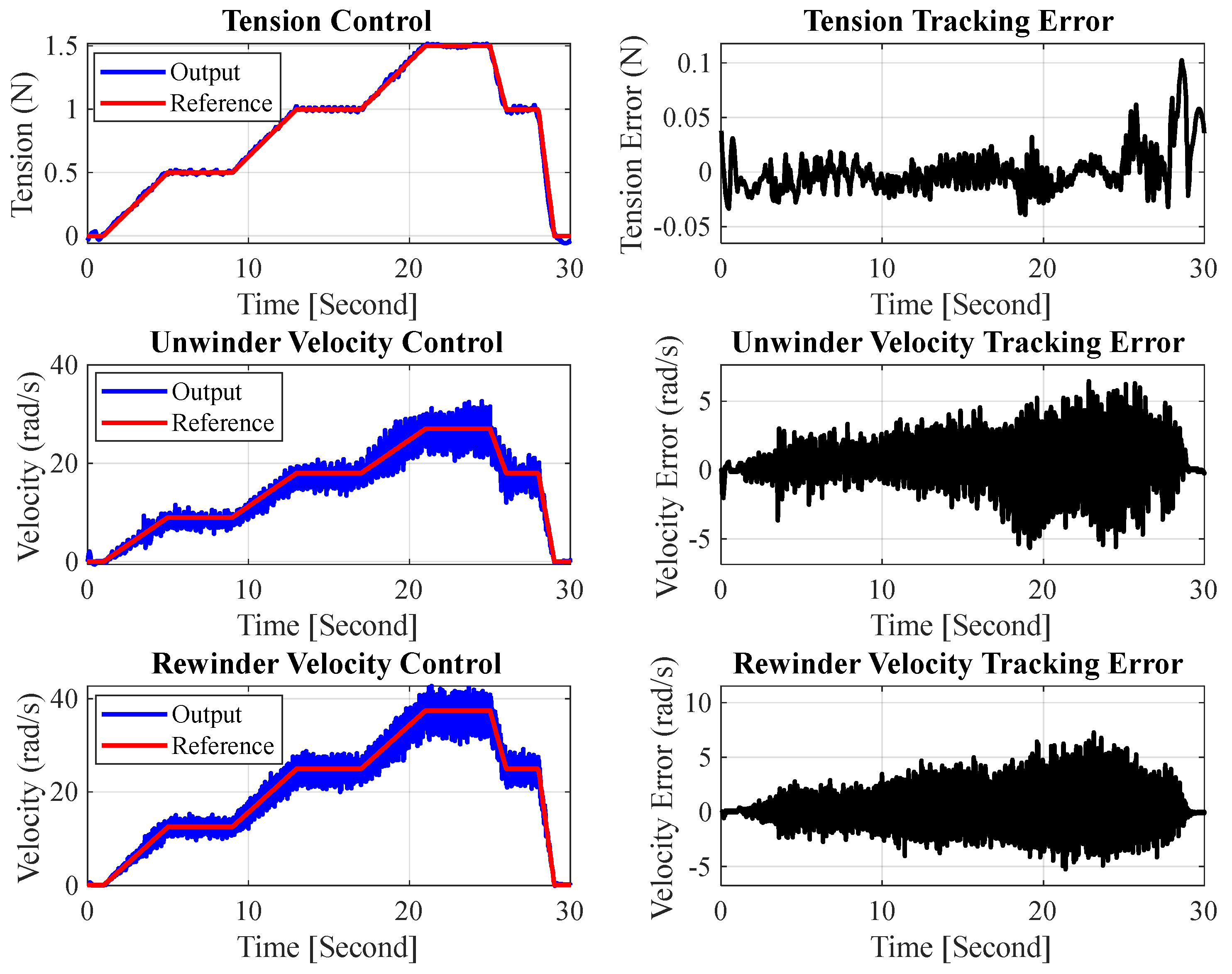
4.1. Controller Performance (Normal Operation)

The cascade architecture was first assessed without state estimation using the Kalman filter (Figure 8). Although radius compensation and inner-loop velocity feedback were active, the raw load-cell signal—plotted in blue—contains pronounced high-frequency noise. This corrupts the tension feedback, resulting in (i) a steady oscillatory error of approximately ±0.5 N around the 1 N setpoint, (ii) a large negative spike at the 22 s reverse-acceleration transient, and (iii) growing error envelopes in both the unwinder and rewinder velocity channels. The right-hand error panels corroborate these observations: the tension error seldom converges to zero and the velocity errors eventually exceed ±10 rad s⁻¹. Hence, the controller alone is unable to guarantee precise tracking when the measurement noise is directly injected into the loop.

Figure 9 repeats the experiment after augmenting the same cascade controller with a discrete Kalman filter. A multi-step excitation—successive 0.25 N tension increments up to 1.5 N followed by symmetrical decrements—was applied to demonstrate performance over an extended operating envelope. The estimated tension aligns with the reference throughout the profile; the steady-state error remains within ±0.02 N and no appreciable overshoot is observed. Both unwinder and rewinder velocities follow their references smoothly, with error magnitudes confined to ±5 rad s⁻¹ despite the continually varying setpoints. The marked reduction in error variance and the absence of large excursions confirm that the Kalman filter effectively attenuates measurement noise, enabling the outer tension loop to exploit the full bandwidth of the inner velocity loops.

Collectively, Figure 8 and Figure 9 highlight the necessity of Kalman state estimation: without it, noise propagates through the hierarchy and degrades regulation; with it, the cascade controller meets the stringent tracking objectives across all three stages—tension, unwinder velocity, and rewinder velocity.

4.2. Fault Detection Performance

The performance of the GPR-based fault detection system was evaluated by deliberately introducing faults during system operation.

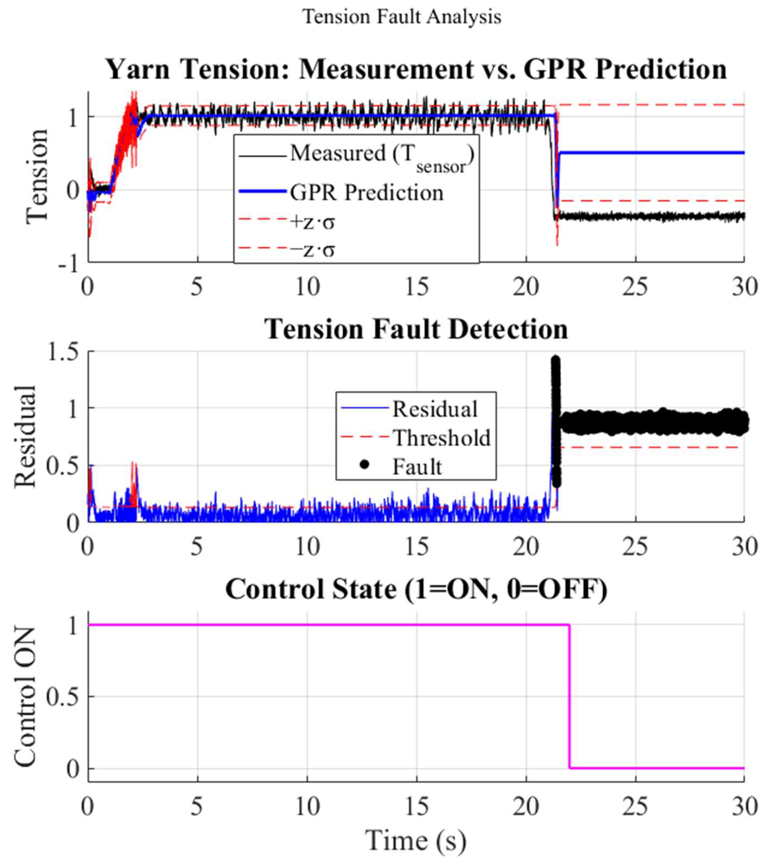
4.2.1. Yarn Breakage Scenario

A yarn break was simulated by manually cutting the yarn during steady-state operation.

In Figure 10 it can be seen that at $t \approx 21$ s, the yarn was severed while the system was in a steady state. The measured tension $T_{Sensor}$ collapsed almost instantaneously to 0 N, whereas the GPR model, driven only by the still-unchanged motor speeds, continued to predict ≈ 1 N. The resultant residual rose from 0.1 N to 1.3 N, surpassing the empirically chosen threshold $T{h}_T$ ≈ 0.5 N within one sampling interval (~50 ms). The supervisory logic therefore asserted a fault flag, and the control enable line was set low (status = 0), preventing any further actuation of the unwinder and rewinder drives. No false positives were recorded in the 10 s pre-fault window, demonstrating adequate robustness of $T{h}_T$.

4.2.2. Unwinder Motor Fault

Power to the unwinder drive was disconnected at t ≈ 15 s (in Figure 11). The measured velocity ${\omega }_u$ jumped from −23 rad s⁻¹ to 0 rad s⁻¹, whereas the GPR predictor, unaware of the electrical failure, continued to output −15 rad s⁻¹. The residual therefore exceeded its limit $T{h}_{\omega u}\approx 7$ rad s⁻¹ almost immediately. Fault declaration again occurred within one sample, prompting an emergency cutoff. The low residual level (<3 rad s⁻¹) observed before the fault indicates that the velocity model captured the nominal dynamics with sufficient fidelity.

4.2.3. Rewinder Motor Fault

An analogous experiment was carried out on the rewinder drive at t ≈ 27 s (Figure 12). Here the measured speed ${\omega }_r$ rose from −20 rad s⁻¹ to +1 rad s⁻¹ while the predictor maintained the pre-fault estimate of −19 rad s⁻¹, yielding a peak residual of ≈ 38 rad s⁻¹. The threshold $T{h}_{\omega r}(\approx 10 rad s{-}^1)$ was breached within 60 ms, and the controller was disabled as before.

5. Discussion

This experimental study demonstrates how estimation and data-driven monitoring jointly elevate both precision and resilience of the roll-to-roll (R2R) line. Below, the main lessons are distilled without retracing the detailed figures already presented in Section 4.

5.1. Analysis of Controller Performance

Noise in the raw load-cell signal had been the dominant barrier to tight tension regulation. Embedding a discrete Kalman filter within the cascade architecture suppresses that noise while preserving the low-frequency dynamics relevant to control action, enabling higher outer-loop gains and smoother inner-loop velocity responses. In effect, the estimator lets the controller operate at the bandwidth dictated by plant physics rather than by sensor quality. The remaining small-amplitude ripples are attributed to unmodelled visco-elastic creep and suggest that future observers could incorporate an additional creep state or deploy an $H\mathrm{\infty }$ design for further robustness.

5.2. Fault Detection Insights

The GPR residual scheme detects yarn and motor faults within a single sampling period and shows no false alarms under nominal operation—performance that meets industrial R2R safety guidelines. Because the GPR learns the coupled dynamics of tension and dual-drive velocities directly from the data, it handles radius variation, friction non-linearities, and other effects that are difficult to capture analytically. Fixed residual thresholds were sufficient here, yet adaptive limits (moving-window tests) would guard against long-term drift in sensor bias or coating thickness.

5.3. Integrated Perspective

The two subsystems are mutually reinforcing: the Kalman filter delivers noise-attenuated states that permit aggressive, high-bandwidth tracking, while the GPR monitor provides a fast safeguard against sudden faults that would otherwise propagate through the tightly coupled web path. The combined architecture therefore addresses both product quality and safety-interlock requirements of modern “smart” R2R lines. Future work should explore incremental or sparse GPR updates for online adaptation, multi-fault classification with specialized residual models, and extension of the observer to include web-stretch dynamics at higher line speeds.

5.4. Comparison with the Literature

Previous roll-to-roll (R2R) investigations that employ cascade control with either disturbance observers or simple low-pass filtering typically report peak steady-state tension errors in the range of 0.02–0.05 N, but only for a single operating point and under modest reference changes [37]. In the present work, the same numerical accuracy is maintained while the reference is swept through six successive levels between 0 N and 1.5 N and subjected to rapid reversals. Because the discrete Kalman filter attenuates the 0–200 Hz noise band without introducing appreciable phase lag, the outer tension loop can exploit the full bandwidth of the inner velocity loops. Consequently, the unwinder and rewinder velocity errors remain confined to ±5 rad s⁻¹—approximately half the magnitude observed in disturbance-observer-based winders of comparable scale—thereby reducing web stretch and improving coat-weight uniformity.

With respect to fault isolation, industrial web lines still rely largely on simple tension drop switches for yarn breaks and analytic observers for drive faults. GPR has been applied to photovoltaic arrays and rotating machinery, yet not to multi-span web handling. The residual monitor introduced here detects yarn breakage and both drive-loss scenarios within a single less than 1 s sampling interval while exhibiting zero false positives during fault-free operation.

6. Conclusions

This study has demonstrated that coupling a model-based cascade controller with a probabilistic, data-driven diagnostic layer can simultaneously achieve high-precision regulation and rapid fault detection in R2R textile systems. The cascade control scheme—strengthened by parameter identification and Kalman-filtered state estimation—maintains prescribed tension and velocity profiles throughout the winding cycle despite continuously changing roll radii. The GPR-based monitor, built from offline healthy-operation data, reliably flags yarn-break and motor-drive faults within one sampling period, without false positives. Together, these subsystems enhance both product quality and process resilience. Moreover, the rapid fault detection and immediate shutdown capability mitigate material loss and equipment damage, reduce unplanned downtime, and support consistent product specifications, thereby delivering significant economic value that offsets the initial investment in industrial-grade hardware, engineering development, and real-time computational resources. This economic viability, combined with the method’s inherent adaptability, underscores its application prospects in continuous manufacturing and lays the groundwork for future extensions such as predictive maintenance.

Future research opportunities include broadening empirical verification by introducing additional fault modes (e.g., web-wrinkle and bearing faults) and testing under varied operating conditions to confirm the GPR detector’s stability and false-alarm resilience; embedding adaptive gain-scheduling or model-reference adaptive control to maintain performance under varying material properties and throughput; developing self-adjusting decision thresholds that leverage the GPR’s predictive variance for dynamic false-alarm management; implementing sparse or incremental GPR training algorithms for online adaptation to slowly drifting system dynamics; extending the diagnostic framework to multi-fault classification and sensor-fault isolation via multi-sensor fusion; exploring hybrid data-driven modeling to improve prediction accuracy and computational efficiency; and validating the approach on industrial-scale R2R lines through digital-twin integration and hardware-in-the-loop testing to ensure real-time determinism. Comparative studies of alternative machine-learning techniques—such as recurrent neural networks and support-vector regression—will further benchmark detection latency, robustness, and computational burden, paving the way for more resilient and scalable “smart” R2R control-and-diagnosis systems.

References

1. Ji, Y.; Ma, J.; Zhou, Z.; Li, J.; Song, L. Dynamic Yarn-Tension Detection Using Machine Vision Combined with a Tension Observer. Sensors 2023, 23, 3800. [Google Scholar] [CrossRef] [PubMed]
2. Haque, M.E.; Kabiraj, R.; Khan, M.M.; Kaiser, M.S.U.; Rahman, M.B. Effect of Machine Parameters on Starting Mark in Textiles Denim Weaving Process. Int. J. Text. Sci. 2023, 12, 1–9. [Google Scholar]
3. Regulating Web Tension in Tape Systems with Time-Varying Radii. Available online: https://ieeexplore.ieee.org/document/5160543 (accessed on 30 April 2025).
4. Ofosu, R.A.; Zhu, H. Tension Control Algorithms Used in Electrical Wire Manufacturing Processes: A Systematic Review. Cogent Eng. 2024, 11, 2322837. [Google Scholar] [CrossRef]
5. Jabbar, K.A.; Pagilla, P.R. Modeling and Analysis of Web Span Tension Dynamics Considering Thermal and Viscoelastic Effects in Roll-to-Roll Manufacturing. J. Manuf. Sci. Eng. 2018, 140, 051005. [Google Scholar] [CrossRef]
6. Lu, J.-S.; Chen, H.-R.; Cheng, M.-Y.; Su, K.-H.; Cheng, L.-W.; Tsai, M.-C. Tension Control Improvement in Automatic Stator In-Slot Winding Machines Using Iterative Learning Control. In Proceedings of the 2014 International Conference on Information Science, Electronics and Electrical Engineering, ISEEE 2014, Sapporo City, Hokkaido, Japan, 26–28 April 2014; pp. 1643–1647. [Google Scholar] [CrossRef]
7. Abd-Elraouf, M.A.; El-Shenawy, A.; Ashour, H.A. Performance Improvement of Automatic Tension Control in Multi Coordinate Drive Systems for Industrial Paper Winder. In Proceedings of the 2017 Nineteenth International Middle East Power Systems Conference (MEPCON), Nasr City, Egypt, 19–21 December 2017; pp. 1163–1169. [Google Scholar]
8. Mokhtari, F.; Sicard, P.; Hazzab, A. Decentralized Nonlinear Control Strategies for Disturbance Rejection in Winding Systems. In Proceedings of the 2011 IEEE International Electric Machines and Drives Conference, IEMDC 2011, Niagara Falls, ON, Canada, 15–18 May 2011. [Google Scholar] [CrossRef]
9. Hwang, H.; Lee, J.; Eum, S.; Nam, K. Kalman-Filter-Based Tension Control Design for Industrial Roll-to-Roll System. Algorithms 2019, 12, 86. [Google Scholar] [CrossRef]
10. Zhong, H.; Pao, L.Y. Feedforward Control to Attenuate Tension Error in Time-Varying Tape Systems. In Proceedings of the 2008 American Control Conference, Washington, DC, USA, 11–13 June 2008; pp. 105–110. [Google Scholar]
11. Sundaram, T.; Velumani, M.M.; Lakshmi, V.S.; Sendhilkumar, S.; Balaji, A.K.; Rajkumar, S.; Seranthian, R. Design and Analysis of Automated Film Roll Cutter. Eng. Proc. 2024, 66, 30. [Google Scholar] [CrossRef]
12. Damour, J. The Mechanics of Tension Control; Converter Accessory Coporation: Wind Gap, PA, USA, 2014; p. 9. [Google Scholar]
13. Peng, C.; Yuan, X. A Study on Detection of Roving Tension and Fine Control of Yarn Breakage. Ind. Textila 2021, 72, 250–255. [Google Scholar] [CrossRef]
14. Azevedo, J.; Ribeiro, R.; Matos, L.; Sousa, R.; Silva, J.; Pilastri, A.; Cortez, P. Predicting Yarn Breaks in Textile Fabrics: A Machine Learning Approach. Procedia Comput. Sci. 2022, 207, 2301–2310. [Google Scholar] [CrossRef]
15. Zhang, H.; Lin, X.; Zhai, Z.; Wu, J.; Zhang, C. A Constant Residual Tension Control Method for the Precision Winding of Yarns. Text. Res. J. 2025, 95, 931–943. [Google Scholar] [CrossRef]
16. Tastimur, C.; Ağrikli, M.; Akin, E. Anomaly Detection in Yarn Tension Signal Using ICA. Turk. J. Sci. Technol. 2023, 18, 33–43. [Google Scholar] [CrossRef]
17. Lee, H.; Lee, Y.; Jo, M.; Nam, S.; Jo, J.; Lee, C. Enhancing Diagnosis of Rotating Elements in Roll-to-Roll Manufacturing Systems through Feature Selection Approach Considering Overlapping Data Density and Distance Analysis. Sensors 2023, 23, 7857. [Google Scholar] [CrossRef] [PubMed]
18. Shao, H.; Peng, J.; Shao, M.; Liu, B. Multiscale Prototype Fusion Network for Industrial Product Surface Anomaly Detection and Localization. IEEE Sens. J. 2024, 24, 32707–32716. [Google Scholar] [CrossRef]
19. Intelligent Diagnosis Method for Early Faults of Electric-Hydraulic Control System Based on Residual Analysis-ScienceDirect. Available online: https://www.sciencedirect.com/science/article/abs/pii/S0951832025003436 (accessed on 9 June 2025).
20. Multi-Objective Maintenance Strategy for Complex Systems Considering the Maintenance Uncertain Impact by Adaptive Multi-Strategy Particle Swarm Optimization-ScienceDirect. Available online: https://www.sciencedirect.com/science/article/abs/pii/S0951832024007427 (accessed on 9 June 2025).
21. Gregorcic, G.; Lightbody, G. Gaussian Process Approach for Modelling of Nonlinear Systems. Eng. Appl. Artif. Intell. 2009, 22, 522–533. [Google Scholar] [CrossRef]
22. He, Z.-K.; Liu, G.-B.; Zhao, X.-J.; Wang, M.-H. Overview of Gaussian Process Regression. Kongzhi Yu Juece/Control Decis. 2013, 28, 1121–1129+1137. [Google Scholar]
23. Neaz, A.; Lee, E.H.; Jin, T.H.; Cho, K.C.; Nam, K. Optimizing Yarn Tension in Textile Production with Tension–Position Cascade Control Method Using Kalman Filter. Sensors 2023, 23, 5494. [Google Scholar] [CrossRef] [PubMed]
24. Chen, Z. Control of High Precision Roll-to-Roll Printing Systems. Ph.D. Thesis, University of Machigan, St, Ann Arbor, MI, USA, 2023. [Google Scholar]
25. Raul, P.; Pagilla, P. Design and Implementation of Adaptive PI Control Schemes for Web Tension Control in Roll-to-Roll (R2R) Manufacturing. ISA Trans. 2015, 56, 276–287. [Google Scholar] [CrossRef]
26. Basu, A.; Gotipamul, R. Effect of Some Ring Spinning and Winding Parameters on Extra Sensitive Yarn Imperfections. Indian J. Fibre Text. Res. 2005, 30, 211–214. [Google Scholar]
27. Tsai, S.-Y. Design and Development of a Web Roll-to-Roll Testing System with Lateral Dynamics Control of Displacement Guide. Ph.D. Thesis, Massey University, Palmerston North, New Zealand, 2012. [Google Scholar]
28. Martin, C.; Zhao, Q.; Patel, A.; Morquecho, E.; Chen, D.; Li, W. A Review of Advanced Roll-to-Roll Manufacturing: System Modeling and Control. J. Manuf. Sci. Eng. 2024, 147, 041004. [Google Scholar] [CrossRef]
29. Lee, J.; Byeon, J.; Lee, C. Theories and Control Technologies for Web Handling in the Roll-to-Roll Manufacturing Process. Int. J. Precis. Eng. Manuf.-Green Tech. 2020, 7, 525–544. [Google Scholar] [CrossRef]
30. Kim, J.; Kim, K.; Kim, H.; Park, P.; Lee, S.; Lee, T.; Kang, D. Experimental Validation of High Precision Web Handling for a Two-Actuator-Based Roll-to-Roll System. Sensors 2022, 22, 2917. [Google Scholar] [CrossRef]
31. Kim, J.; Kim, H.; Kim, K.-R.; Kang, D. Dynamics and Control of Web Handling in Roll-to-Roll System With Driven Roller. IEEE Access 2023, 11, 58159–58168. [Google Scholar] [CrossRef]
32. Zheng, D.; Pryor, M. Control of High Precision Roll-to-Roll Manufacturing Systems. Ph.D. Thesis, The University of Texas at Austin, Austin, TX, USA, 2018. [Google Scholar]
33. Liao, Y.; Xie, J.; Wang, Z.; Shen, X. Multisensor Estimation Fusion with Gaussian Process for Nonlinear Dynamic Systems. Entropy 2019, 21, 1126. [Google Scholar] [CrossRef]
34. Julier, S.J.; Uhlmann, J.K. A New Extension of the Kalman Filter to Nonlinear Systems. Ph.D. Thesis, The University of North Carolina at Chapel Hill, Chapel Hill, NC, USA, 1997. [Google Scholar]
35. Maffioletti, F. Data-Driven Techniques for Printer Prognosis and Performance Improvement: Design and Critical Comparison. Ph.D. Thesis, Delft University of Technology, Delft, The Netherlands, 2019. [Google Scholar]
36. Saeidi-Javash, M.; Wang, K.; Zeng, M.; Luo, T.; Dowling, A.W.; Zhang, Y. Machine Learning-Assisted Ultrafast Flash Sintering of High-Performance and Flexible Silver–Selenide Thermoelectric Devices. Energy Environ. Sci. 2022, 15, 5093–5104. [Google Scholar] [CrossRef]
37. Robust Tension Control of Roll to Roll Winding Equipment Based on a Disturbance Observer. Available online: https://www.researchgate.net/publication/312113489_Robust_tension_control_of_roll_to_roll_winding_equipment_based_on_a_disturbance_observer (accessed on 30 April 2025).
Figure 1. Experimental System Hardware Setup.
Machines 13 00548 g001
Figure 2. System dynamics of the roll-to-roll system.
Machines 13 00548 g002
Figure 3. System identification of unwinder and rewinder rollers.
Machines 13 00548 g003
Figure 4. Experimental results of yarn system identification.
Machines 13 00548 g004
Figure 5. Overall control architecture of the experimental system.
Machines 13 00548 g005
Figure 6. Result of noise processing with the Kalman filter and low-pass filter.
Machines 13 00548 g006
Figure 7. Data collection and model training pipeline for the R2R fault detection system.
Machines 13 00548 g007
Figure 8. Cascade controller performance without Kalman filtering.
Machines 13 00548 g008
Figure 9. Cascade controller performance with Kalman filtering.
Machines 13 00548 g009
Figure 10. Yarn-break test: measured vs. GPR tension, residual with threshold, and control cutoff.
Machines 13 00548 g010
Figure 11. Unwinder motor fault: measured vs. GPR speed, residual with threshold, and control cutoff.
Machines 13 00548 g011
Figure 12. Rewinder motor fault: measured vs. GPR speed, residual with threshold, and control cutoff.
Machines 13 00548 g012