Abstract
Arc welding is a complex multiphysics mitigation process, and the related finite element simulation requires significant computational resources for multiphysics modeling to determine the temperature distributions in engineering problems accurately. Engineers and researchers aim to achieve reliable results from finite element analysis while minimizing computational costs. This research extensively studies the application of conventional ellipsoidal heat source formulation to obtain improved temperature distribution during arc welding for practical applications. The ellipsoidal heat source model, which artificially modifies the coefficient of thermal conductivity in the welding pool area to simulate stirring effects, is proven to be scientifically valid by comparing its results with those of COMSOL’s multiphysics arc welding analyses. The findings from finite element analyses demonstrate that the temperature fields generated using the modified ellipsoidal approach exhibit strong agreement with those obtained from multiphysics simulations, especially within the core regions of the weld pool. The method can easily be implemented in all different welding methods in which a stirring effect is formed by either electromagnetic or buoyancy-driven flows in the weld pool area. Furthermore, the method offers computational efficiency without sacrificing accuracy, making it suitable for industrial applications where multiphysics modeling is not feasible but reliable thermal and structural predictions are essential.
1. Introduction
Since welding methods were invented in the early 1900s, these methods have been advanced and used for various materials in enormous engineering mitigation problems. In weld design applications, calculating the correct stress and temperature distribution in a welded part is extremely important. Therefore, engineers are eager to use every effective experimental and numerical method possible in the welding area. According to historical perspectives, it is true that the finite element (FE) is one of the most widely used numerical techniques in weld design analyses. Mainly, FE welding analysis can be performed in two ways. One way is a simple transient thermal elastoplastic FE analysis, and the second way is a multiphysics analysis to determine the stress and temperature distribution in and around the weld region.
Up to now, several researchers, have investigated the multiphysics welding phenomena intensively. Meanwhile, various commercial software is also available (COMSOL V5.5 Multiphysics Stockholm, Sweden, etc.) in the market, and they provide good results for even highly complicated multiphysics cases in welding analyses. However, multiphysics solutions require extremely large computational costs for even simple 2D analyses because FE analysis of the welding process consists of engineering disciplines such as electricity, magnetism, CFD, heat transfer, and solid structure in a couple. Additionally, in many large-scale steel construction areas, design engineers need much simpler FE models that require less computational cost unless they have extremely powerful computers. For this reason, searching for a simple and effective way of FE welding analysis goes back to the early 1980s.
In 1971, Udea et al. [1] showed that the FE procedure could be used in coupled or uncoupled transient thermal elastic–plastic FE analysis. However, this kind of analysis model needs an appropriate heat source formulation to simulate the welding process. According to the literature, various heat source formulations are proposed and used in FE welding analyses. If these heat source formulations are ordered from simple to complex ones, the first example is research conducted by Chau et al. [2]. In this research, the authors propose uniform specific temperature usage, not only for the weld bead region, but also for a couple of surrounding regions in a regional way to simulate the process. Although the method employs a constant melting temperature distribution within the weld bead and the surrounding heat-affected zone to mitigate the severe temperature gradient, it fails to achieve an acceptable temperature distribution in the weld region.
Subsequently, Rosenthal [3] introduced a simplified point heat source model in 1946. While this formulation generally yields satisfactory results for areas sufficiently distant from the weld region, it predicts an infinite temperature at the source center, which is not physically realistic. To address this limitation, Pavelic et al. [4] proposed a Gaussian-distributed surface heat source model, offering improved accuracy in temperature distribution compared to Rosenthal’s model. However, this model is effective only in cases involving shallow weld penetrations, as the heat source is applied exclusively to the surface, thereby limiting its ability to model deeper welds.
Finally, Goldak et al. [5] introduced a significant advancement with a volumetric heat source model, which combines two ellipsoids representing the front and rear halves of the heat source. This double-ellipsoid model provides a more accurate representation of heat distribution within the weld region compared to earlier models and has been widely adopted by researchers and integrated into several commercial finite element software packages, becoming the de facto standard in the field.
Numerous good examples can be given from recent research. One of them is Kollár’s work [6]. In this research, the author deals with T-joints with fillet welds commonly used in civil engineering applications with Goldak’s method and investigates the impact of correcting the lack of penetration by repair welding concerning distortions and residual stresses. The research emphasizes the importance of the double-ellipsoid method in welding simulation and avoids repair welding by finding the resultant plastic strain and von Mises residual stress, which increased significantly due to rewelding.
In a separate study conducted by Obeid O et al. [7], the authors examine the influence of girth welding materials on welded lined pipes through both numerical simulations and experimental investigations, incorporating a sensitivity analysis. Thermal and mechanical finite element (FE) models are developed using FORTRAN subroutines in conjunction with ABAQUS 2022 software, with pre-heat treatment conditions applied as the initial parameters. In the experimental component, high-temperature strain gauges, residual stress gauges, and X-ray diffraction techniques are employed to measure strains and residual stresses along the inner and outer surfaces of the welded lined pipe. These measurements are correlated with the recorded thermal history to provide comprehensive insights into the welding process. However, these models have some weaknesses related to heat distribution in the weld region. Firstly, the weld pool’s shape must be ellipsoidal in this model. If the shape of the weld pool is non-ellipsoidal, the heat source equation must not be used properly. Secondly, the stirring phenomena in the molten metal flow occurring during welding are ignored. Therefore, especially in the weld fusion zone (FZ), if the temperature distribution is not determined as close as to reality, related residual stress calculations significantly deviate from the correct values, as clearly seen in Ref. [7], in the weld pool region. Therefore, high-level calculations do not give good estimations, such as those in crack propagation inside the fusion zone (FZ), which is highly important for providing the required safety, especially in nuclear industries. Goldak et al. [5] recommend artificially increasing the heat conduction coefficient at nodal points where the temperature exceeds the melting point. However, this approach is insufficient to adjust the heat distribution in the pool region to ensure all nodal temperatures reach the melting point. Nart et al. [8] proposed a new method of implementing Goldak’s heat source, replacing the previous nodal-based approach of increasing the thermal conductivity in welding analysis with an area-based approach. According to these authors’ research, the proposed approach shows an improvement in the history of the temperature in the FZ because the corresponding residual stress obtained from finite element simulation and X-ray measurement are extremely close to each other. Although the results of Nart et al.’s work are meaningful, it is necessary to prove whether this experimental observation has a physical basis to proceed further.
Therefore, multiphysics welding models are closely investigated in this research. It is known that various kinds of research are available that can be used to model welding phenomena realistically—some of these models in the literature deal with arc plasma modeling.
For example, Wu et al. [9] investigate plasma physics and its properties to optimize the performance of Tungsten Inert Gas (TIG) welding by simultaneously solving the conservation equations for mass, momentum, energy, and electric current. The authors develop a mathematical model to predict the distributions of velocity, temperature, and current density within argon welding arcs. Similarly, Hsu et al. [10] present solutions to the conservation equations for the entire free-burning arc, excluding the cathode and anode fall regions. The most critical boundary condition—current density near the cathode—is derived from measurements of the molten cathode tip size. The calculated temperature fields within the arc are validated through spectrometric measurements, utilizing both line and continuum intensity data from the arc.
These researchers focus exclusively on the arc plasma region to calculate the temperature distribution and gas velocity fields within the plasma. Their studies specifically investigate phenomena such as heat and current transfer, as well as the arc pressure and its associated drag force at the outer boundary near the weld pool. This targeted approach is essential, as arc welding phenomena cannot be accurately modeled when the arc plasma and molten pool are considered in isolation. Consequently, advanced models that integrate the conservation equations with selected Maxwell’s equations, alongside appropriate boundary conditions, are required to more accurately represent Marangoni-driven flows.
For this reason, researchers have been extensively exploring new methodologies to model the multiphysics nature of the TIG welding process. Tanaka [11] investigates both the plasma and molten pool simultaneously, accounting for all the driving forces that influence convective currents within the molten pool during TIG welding. The study considers the drag force exerted by the plasma jet, the buoyancy force, the electromagnetic force generated by current flow in the molten pool, and the Marangoni effect, which arises from surface tension gradients. Tanaka’s findings demonstrate that the formation of the molten pool is governed by the interplay of heat transfer and macro-convection within the molten region. Ultimately, the study concludes that the precise formation of the molten pool is dictated by a delicate balance among these four forces.
In another research paper, Tanaka et al. [12] introduce a review of methodologies for predicting the properties of the arc and also the profile of the weld pool produced by the arc. The authors consider two electrodes in the modeling, i.e., cathode and anode, in which the electrode surfaces are needed in modeling for effects of energy and momentum transfer at the electrodes. The researchers also noticed that the temperature dependence of the surface tension coefficient has a marked effect on weld depth and profiles because it can influence the direction of circulatory flow in the weld pool. Tanaka et al., remarkably, realize that electric arc in different inert gases affects the weld pool shape as a consequence of the magnetic pinch pressure of the arc.
In his dissertation, Tradia [13] studies mathematical modeling and numerical simulation of the arc welding process for both stationary and moving cases using GTAW. In the research, the author focuses on a 3D arc welding model considering the welding position and the effect of the filler material used to investigate the GTAW process. The welding process is considered in pulsed current mode by using different gas mixtures, and the effect of welding parameters on the resulting weld shapes is investigated.
Recently, Li et al. [14] developed a useful method to calculate the keyhole PAW process with full consideration of multiphysical mechanisms. The paper investigates weld pool size with different solid viscosity and mushy zone constant. The model is useful to give a good prediction of weld pool geometry at proper welding conditions. The mathematical model was solved by the software Fluent with user-defined functions and user-defined scalar equations.
Farias et al. [15] introduce an inverse optimization strategy that integrates genetic algorithms with a reduced geometry approach to identify optimal heat source parameters while significantly minimizing computational effort. Their method was applied to distinct joint configurations and base materials, incorporating temperature-dependent properties and various heat transfer mechanisms within ANSYS® 2021 R2 Multiphysics® simulations. Expanding upon this, Farias et al. [16] propose novel heat source models based on the observed morphology of the fusion zone (FZ) in macrographic images. These models aim to more accurately reflect the thermal gradients surrounding the weld pool, surpassing the limitations of conventional models that rely solely on the heat conduction equation. The new formulations are evaluated against classical conical models and Goldak’s double-ellipsoidal heat source representation.
Karganroudi et al. [17] enhance the modeling framework by integrating a non-uniform, moving volumetric heat flux into the finite element analysis through a custom DFLUX subroutine written in FORTRAN. Their study employs Response Surface Methodology (RSM) to statistically assess the influence of key TIG welding parameters on weld bead width and penetration depth for 1.4418 stainless steel. Using Derringer’s desirability function, they further identify optimal process parameters for multi-objective optimization.
In a related effort, Moslemi et al. [18] focus on the accurate prediction of Goldak’s heat source parameters using a data-driven methodology. A three-dimensional finite element model generates a dataset of weld pool characteristics, which are then analyzed using both linear and quadratic regression models, as well as Artificial Neural Networks (ANN). The comparative results demonstrate that ANN-based models offer superior accuracy in capturing the thermal behavior of the weld pool.
In this research, a dimensionally simplified multiphysics TIG welding model is implemented. It is well known that a multiphysics model for welding has several different partial differential equations to be solved simultaneously. This highly nonlinear problem is extremely difficult to solve because the procedure cannot be computed in parallel computers. Therefore, axisymmetric finite element models can be used as a special case for double-ellipsoid heat sources. However, the method used in this research must be extended to the 3D welding problem to prove that modified double-ellipsoidal models can also provide engineers with useful results.
In light of this, multiphysics TIG welding analysis is accordingly performed and the obtained results are compared with the results of the modified ellipsoidal heat source model. The work presented shows that an approximated ellipsoidal heat source model that artificially changes the coefficient of thermal conductivity in the welding pool area is a scientifically acceptable method by comparing the results of both ellipsoidal approximate heat sources (modified and conventional) and the COMSOL V5.5 multiphysics arc welding model.
2. Mathematical Formulation and Governing Equations
2.1. Equation for Thermal Plasma Modeling
Plasma is simply a superheated matter that is so hot the electrons are ripped away from the atoms, thus forming an ionized conductive fluid. Therefore, plasmas can be modeled using the magnetohydrodynamics (MHD) equations. It is well known that MHD uses the Navier–Stokes, heat, and Maxwell’s equations to define the motion of the conducting fluid in an electromagnetic field. Subsequently, these governing equations determine the fluid motion of the plasma after suitably solving the equation. However, the plasma generated by the arc can reach high velocities due to thermal expansion and the electromagnetic forces acting on charged particles. The speed of the plasma can often exceed 0.3 Mach, particularly in the central regions of the arc, where temperature and energy are highest. Consequently, these conditions within the arc can lead to compressible flow characteristics and deviations from local thermodynamic equilibrium (LTE) in regions with strong velocity and density gradients. Similarly, other non-equilibrium conditions also occur in plasmas; for example, radiation emitted from the plasma disrupts the detailed balance as it escapes the plasma.
However, in high-temperature plasmas and rapidly moving gases, frequent collisions among particles can help maintain local equilibrium in small volumes, making the LTE assumption valid. This is possible because collisions allow particles to quickly share energy levels. On the other hand, concerning radiation processes, electrode heating from arc radiation can generally be ignored when a sufficiently high electron density is present. However, on the electrode surface, the cooling effect due to thermionic emission should be included in the calculations.
In the field of welding, the LTE assumption is commonly used to model the behavior of the plasma arc. This approach allows for an approximate understanding of local thermodynamic properties to analyze the heat transfer, melting processes, and interaction between the arc and the workpiece. Additionally, the LTE assumption is typically employed as a starting point, enabling researchers to focus on primary interactions without getting overly involved in the complexities of non-equilibrium effects.
On the other hand, although the speed of the plasma can often exceed 0.3 Mach and this causes compressible flow in the arc plasma, assuming incompressibility for plasma in welding arcs is often a reasonable approximation for simplifying the governing equations and is commonly used in theoretical models and simulations. For example, Lowke’s paper [19], “Simple theory of free-burning arcs”, presents an analytical framework for understanding the behavior of free-burning arcs, which are commonly observed in welding and related plasma systems. The models in the paper incorporate simplified assumptions to make analytical solutions possible, such as considering steady-state conditions and approximations. Lowke et al. find that in arc welding, when the arc current is relatively below 30 A, the inertia force associated with the plasma becomes more relevant. At these lower currents, the plasma may exhibit noticeable motion due to inertia, which can influence the arc behavior.
However, as the current extends beyond 30 A, the situation changes. The electromagnetic forces generated by the current (Lorenz force) become significantly stronger than the inertia forces. This is because the current generates a magnetic field that interacts with the plasma, exerting a force that tends to push the plasma along the arc. In light of this knowledge, assuming incompressibility for plasma in welding arc is a good opportunity to simplify the modeling.
Therefore, for the modeling of arc plasma in this research, the following assumptions are used [13]:
Assumptions:
- I.
- The arc is in local thermodynamic equilibrium (LTE).
- II.
- Axisymmetric Spot GTA welding is assumed.
- III.
- Pure argon is used and the metal vapors are not considered.
- IV.
- Gas plasma is incompressible and the flow is laminar.
- V.
- Boussinesq approximation is not assumed in plasma.
Based on these assumptions, the conservation equation expressed in terms of axisymmetric case is written as:
or Equation (1)
where is the velocity vector, , and are the axial and radial velocity components, and ρ is the mass density, respectively. and represent the axial and radial volumetric forces. Additionally, the momentum equations are written as follows:
In addition, in the plasma region, the axial volumetric force is defined as the sum of Lorentz and inertia force:
in which is the gas density and the gravity force is included for taking into account the action of buoyancy in the arc plasma domain. In addition, the radial volumetric force is the Lorentz force in Equation (4) and is defined as follows:
In these equations, p, μ, Jr, Jz, and Bθ are the pressure, the viscosity, the radial and axial current density, and the self-magnetic field, respectively [13]. Above, in Equation (3), the self-induced magnetic field can be written as
There is another way to obtain that is used in COMSOL V5.5. The magnetic potential equations are
Subsequently, the current continuity equation is simply obtained from Gauss’s law as follows:
or
and formulated as a function of the electric potential ϕ as follows:
or
where is the electrical conductivity. Ohm’s law yields
Finally, the energy conservation equation takes the form
But in the plasma region, the volumetric heat source consists of the Joule effect, the electrons enthalpy , and the radiation losses, as follows:
where T, Cp, k, kB, e, and are the temperature, specific heat at constant pressure, thermal conductivity constant, the Boltzmann constant, elementary charge, and volumetric heat sources, respectively. Additionally, is the approximated radiation loss taken as 4πЄN, where ЄN is the argon net emission coefficient changing with temperature.
Furthermore, the energy equation consists of convection, conduction, Joule-heating, and electron enthalpy terms (because of electron-ion collision in the anode). The corresponding coupled governing equations are highly nonlinear systems of partial differential equations and the solution is reached by solving them simultaneously.
In this research, COMSOL V5.5 software is used to model and solve these equations by using its strong multiphysics features. In the COMSOL V5.5 environment, one can define all partial differential equations and boundary conditions, and make proper connections among them in couple to solve problems. In this paper, COMSOL V5.5’s implementation of partial differential equations and multiphysics cupping conditions mentioned above can be listed as: Electrical Current, Magnetic Fields, Heat Transfer in Fluids, Laminar Flow, and Heat Transfer in Solids. On the other hand, various interfaces can be easily used in multiphysics modeling and simulations. For instance, the Magnetic Fields interface can be used to solve Ampère’s law. The Equilibrium DC Discharge interface can then be employed to analyze equilibrium discharges induced by static or slowly varying electric fields. This interface operates under the assumption that the plasma is fully ionized, is in a state of local thermodynamic equilibrium (LTE), and the induction currents are negligible. In addition, the Equilibrium Inductively Coupled Plasma interface is designed to evaluate equilibrium discharges resulting from induction currents, as observed in inductively coupled plasma torches. Alternatively, the Combined Inductive/DC Discharge interface facilitates the assessment of equilibrium discharges arising from both induction currents and static or slowly varying electric fields, making it particularly suitable for applications such as arc welding simulations (Equations (1)–(6)). For thermal and fluid dynamics analyses, the Heat Transfer and Laminar Flow interfaces are available to solve the energy equation and the Navier–Stokes equations, respectively. Importantly, multiphysics coupling terms play a critical role in effectively linking these equations, ensuring accurate simulation of the interdependent physical phenomena.
Electrode and Anode Surfaces:
Meanwhile, the positive ions within the plasma contribute to heat generation at the electrode surface. As the electrode temperature rises, an increased number of electrons are emitted via thermionic emission, leading to a cooling effect on the cathode. Consequently, for points along the electrode surface, it is essential to account for both the cooling effect induced by thermionic emission and the heating effects resulting from ion current and thermal conduction in the calculations. In addition, the hypothesis that cathode heating is governed by is substantiated by the experimental findings of researchers in [20,21,22]. These experiments indicate that the entire ionization potential is imparted to the cathode without any diminution by , as the electron required for ion neutralization is supplied from within the cathode surface. Furthermore, for simplicity, it is assumed that the heating of the electrodes due to arc radiation is negligible. For the cathode, the additional energy flux to the electrode, denoted as FElectrode, is expressed as follows:
where ε represents the emissivity of the electrode surface, T denotes the surface temperature, is the work function of the material, and and correspond to the electron and ion current densities, respectively, α is the Stefan–Boltzmann constant, and signifies the ionization potential of the plasma [23].
The ion current density norm is defined by
where is the normal current density at the interface and where
is the electron current density norm. The latter is defined by the Richardson–Dushman current density if the total normal current density is larger than
where denotes Richardson’s constant, e represents the elementary electronic charge (C), is Boltzmann’s constant, and corresponds to the effective work function of the surface. It is important to note that the ion current density becomes zero if the Richardson–Dushman current density exceeds the total normal current at the interface [24]. At the anode surface, the sign of the term in Equation (15) is reversed to reflect the positive heating effect associated with electrons absorbed at the anode. In this context, represents the work function of the anode material.
The anode, which is typically represented by the workpiece, constitutes a distinct region within the arc plasma due to its function in receiving electrons emitted from the cathode. This relatively thin layer operates as an electron-absorbing zone, thereby maintaining electrical continuity between the workpiece and the arc column. As electrons are emitted from the cathode and subsequently accelerated through the arc column, they collide with the anode surface, transferring their kinetic energy to the workpiece. This process is known as electron condensation heating, and it contributes significantly to the thermal energy input of the workpiece through both the arc plasma and the incident electron flux.
However, with regard to radiative effects, the heating of the anode due to arc radiation can generally be considered negligible. Studies in the literature report that the contribution of radiative heat flux to the anode constitutes less than 5% of the total heat input. Nonetheless, for accurate thermal modeling of the anode surface, it is essential to incorporate the cooling effects resulting from thermionic emission into the calculations.
For this reason, the additional energy flux, FAnode, to the anode [25] is taken as
Under the assumption of local thermodynamic equilibrium (LTE), the electron density is equal to the total density of positive charges, thereby maintaining charge neutrality. On the other hand, the presence of electrodes introduces effects that cause local imbalances between negative and positive charges, leading to non-LTE conditions. When the regions near the anode surface are extremely thin, which is approximately 1.5 μm in a 200 A-argon arc, non-equilibrium conditions in charge densities occur.
2.2. Equation for Weld Pool Modeling
The fluid flow occurring in the anode region is defined by the conventional conservation equations of mass and momentum. These conservation equations can be written in a time-independent form in Equations (20)–(22) with respect to the assumptions given below. In addition, the solution for the electromagnetic problem in the anode and cathode domain is needed to calculate the Lorentz forces and Joule effects for heating. These Lorentz forces and Joule effects for heating are governed by the classical Maxwell’s equations given previously.
Assumptions:
- I.
- Axisymmetric Spot GTA welding is assumed.
- II.
- The metal flow in the weld pool is laminar.
- III.
- The surface tension coefficient is dependent on both temperature and sulfur content.
- VI.
- The latent heat of fusion is also taken into account.
- V.
- Boussinesq approximation is assumed in the weld pool.
The conservation equations for the weld pool is
or
The momentum equations are
In the anode region at the liquid phase (weld pool), the axial volumetric force consists of Lorentz and inertia force, and the buoyancy force, as follows:
In the above equations, is the melted metal density in the weld pool as the reference. The radial volumetric force is the Lorentz force
Additionally, two more sources of radial momentum exist at the liquid surface of the weld pool. The first is the drag force caused by the shear stress due to the convective flow of the cathode jet on the surface of the weld pool. This drag force is already included in Equation (22) through the viscosity at the weld pool surface. The second is the Marangoni effect due to the gradient in the surface tension at the surface of the weld pool. This force usually occurs due to temperature differences between the center of the weld pool and the edge of the weld pool. Moreover, these effects can also occur due to changes in the chemical composition of the liquid steel. The additional term for Equation (22) at the weld pool surface is
The temperature coefficient of surface tension for pure metals is typically negative. However, the presence of impurities such as sulfur in the weld pool can alter this coefficient, resulting in a positive value. In cases where is positive, the direction of the surface stress induced by the Marangoni effect is reversed, leading to significant changes in the flow dynamics within the weld pool. This alteration in surface tension-driven flow subsequently influences the geometry and morphology of the weld pool.
In invaluable research, Sahoo et al. [26] show that the surface tension as a function of both temperature and sulfur activity is obtained as
and by differentiating Equation (26) with respect to temperature, the expression of as a function of both temperature and sulfur activity can be written as follows:
The related values for the coefficients are given in Table 1. Furthermore, the terms in the energy conservation equation are expanded for the anode (workpiece) and cathode region (electrode), and the volumetric heat source term consists of the Joule effect and the radiation losses, as follows:

Table 1.
Material properties of workpiece metal (anode, 304 SS material).
In the same equation, is another term for the radiation loss, as follows:
where is the emissivity of the surface, is the surface temperature, is the Stefan–Boltzmann constant. Furthermore, is an equivalent specific heat, which corresponds to in the arc plasma and cathode regions, and is recalculated for the workpiece (anode) domain taking into account the latent heat of fusion , as follows:
In the meantime, a linear change in temperature is assumed for the liquid fraction fL, as follows [27]:
where TS and TL are the solidus and liquidus temperatures of metal, respectively. The variables and constants with units are given in Table 2.
Table 2.
Physical variables and constants.
3. Computational Domain and Initial Conditions
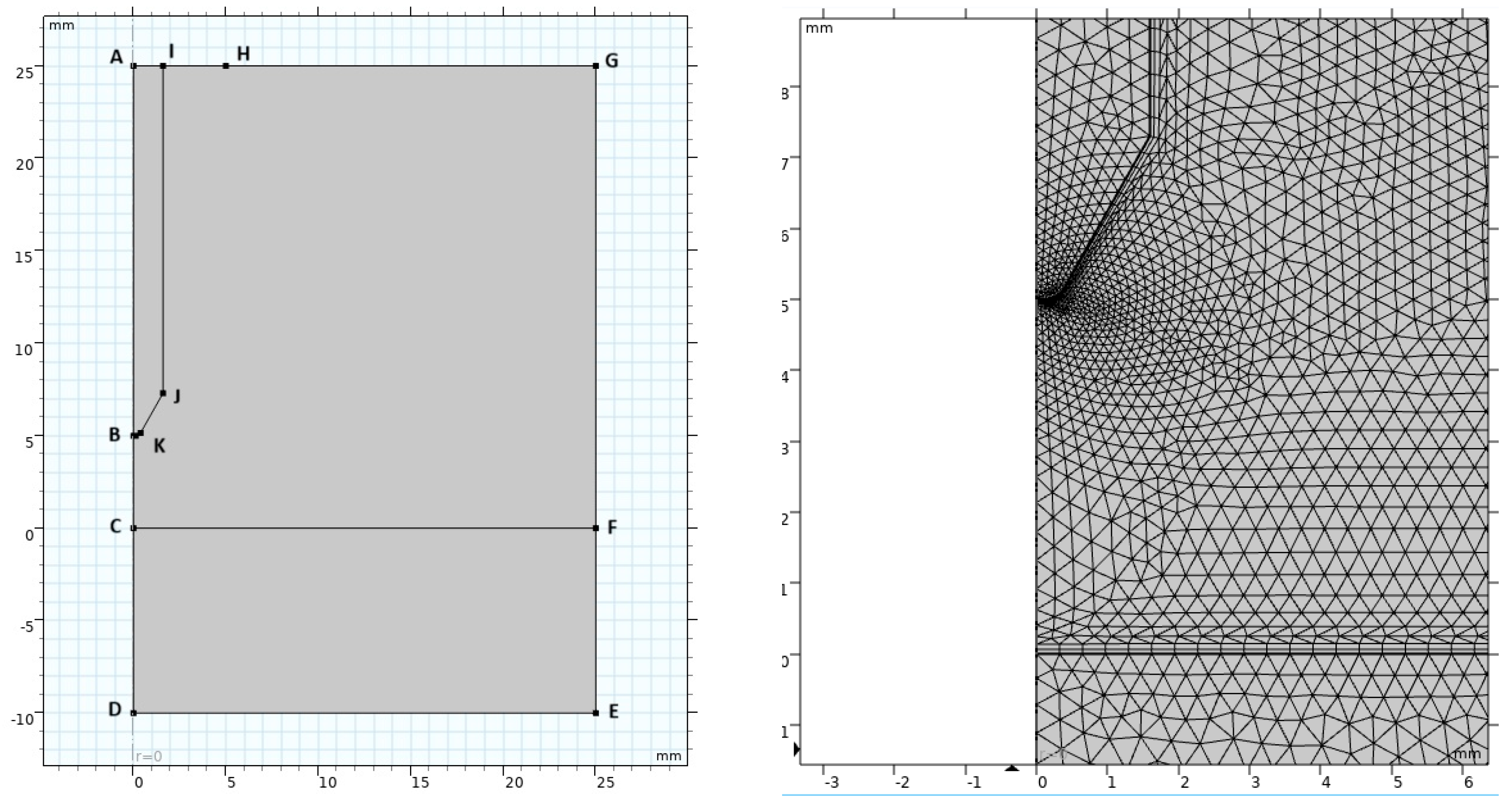
To define the corresponding domains for the governing equations and suitable boundary conditions for this research, the geometry is divided into three subdomains with different mesh densities in each one (Figure 1). For this reason, ABKJI, CDEF, and BCFGHI polygons are formed for the cathode (tungsten electrode tip angel 60-deg), anode (304 stainless steel—medium sulfur content), and arc plasma regions, respectively. For the arc plasma part of the problem, the temperature distribution is computed in the arc plasma and anode domains; however, the fluid flow is computed in the arc plasma domain only [10].
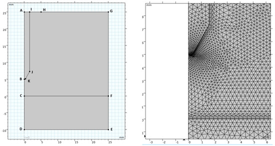
Figure 1.
Finite element model and its dimensions (mm).
In the plasma physics and MHD modeling, the electromagnetic, energy conservation, mass, and momentum conservation equations are solved in the workpiece domain shown in Figure 1, according to the boundaries indicated in Table 3.
Table 3.
Boundary conditions for all studies.
On the other hand, for the modified and conventional ellipsoid models, the heat transfer partial differential equation is solved. In order to do this, the symmetry boundary condition along the DC line was defined as zero heat flux based on the boundaries shown in Figure 1. The ellipsoid heat source was defined along the CF line, with the DC line set as r = 0. Additionally, due to the high heat generation along the same line, heat loss via radiation was also incorporated. Convective heat boundary conditions were applied along the DE and EF lines, allowing heat exchange with the ambient temperature. In the transient heat transfer analysis, the initial temperatures were assumed to be at room temperature, set at 20 °C. All the required boundary conditions for the finite element analyses performed are given explicitly in Table 3.
In addition, this study revealed that the number of mesh elements is crucial in multiphysics analyses. If an insufficient number of mesh elements is used, the multiphysics solution fails to converge accurately. The meshing process must be appropriately tailored to the entire system of partial differential equations being solved. Therefore, in the multiphysics analysis, the mesh density was increased to refine the solution. The weld pool dimensions obtained with the selected mesh configuration were compared with both the experimental results and literature data, confirming that an optimal mesh had been established. Additionally, the same mesh configuration was applied in analyses using the conventional ellipsoid model.
3.1. The Free Surface Deformation
Because of the arc pressure, surface tension, and gravitational force acting on the weld pool, the linear form is lost on the free surface of melted metal in the weld pool. The arc voltage and welding current directly affect the degree of this related deformation. Therefore, the behavior of the liquid/solid interface should be investigated more closely and necessary assumptions should be properly determined.
In reality, in high-current welding applications, the ejected metal droplets deform the pool surface, and the impact and pressure effects of these droplets establish an equilibrium state with the gravitational field, forming an interfacial region. The predicted transition current required for this phenomenon has been determined as 240 A by Ushia [28] (Ushio [16]). Since the current used in this study is 150 A, it remains well below this threshold value.
For this reason, it is concluded that the free surface deformation occurs reasonably small in the course of the process with respect to that of other welding processes. Therefore, it is assumed that the free surface is flat for all MHD calculations.
3.2. The Liquid/Surface Interface
Within the welding pool, an additional interface exists between the liquid and solid phases of the metal. This liquid/solid interface is typically defined by the contour corresponding to the liquidus temperature. Methods employed in weld pool simulations to account for this interface are generally classified into two categories: moving grid methods and fixed grid methods. In the fixed grid approach, the mesh for the pool domain is generated once, and the liquid/solid interface is determined using the liquid fraction function, fL(T). Since the momentum equation is solved across the entire domain, it is necessary to ensure that the velocity field remains zero in the solid region. To achieve this, the Karman–Kozeny approximation and the enhanced viscosity method are commonly applied. In the present study, the enhanced viscosity method is utilized, as described in Equation (33).
In the moving grid methods, the interface for liquid/solid is tracked with time to generate two distinct sub-regions for the melted and solid metal zones at each time step.
3.3. Initial Conditions in the Arc Plasma Region
An electric arc is fundamentally a form of electrical discharge initiated through ionization when the current across the electrodes exceeds the breakdown voltage. This critical breakdown voltage across the electrode gap is influenced by factors such as the surrounding gas pressure, the inter-electrode distance, and the type of gas present. Typically, an electric arc is initiated by bringing two electrodes into contact and then gradually separating them. The electrical resistance along the resulting continuous arc generates heat, which further ionizes the surrounding gas molecules, progressively transforming the gas into a thermal plasma. This mechanism allows for the initiation of an arc without requiring a high-voltage discharge. A similar process occurs during welding, where the welder briefly touches the welding electrode to the workpiece before withdrawing it to establish a stable arc. However, the physical actions of touching and withdrawing electrodes cannot be directly modeled within a fixed mesh computational domain. To address this limitation, an appropriate numerical modeling technique must be employed. This is achieved by imposing a numerically conductive channel between the electrodes. The variation in electrical conductivity within this channel can be effectively represented using an exponential decay function, which facilitates the accurate simulation of arc initiation by defining
In this way, electrical conductivity at r = 0 is artificially increased and the arc is initiated for suitable constant values of A and B.
4. Implementation in COMSOL
COMSOL V5.5 software is utilized to solve all couple governing equations modeling the multiphysics arc welding problem. For this reason, all the governing equations are defined by suitable components with their multiphysics couplings and interfaces. Mainly, the overall simulation procedure can be summarized as follows. In each time increment, the magnetic and electric potentials are computed primarily in the whole domain. Then, the electric field, current density, and magnetic induction are calculated. Next, for calculating the related temperature field, the Joule heat source values are used.
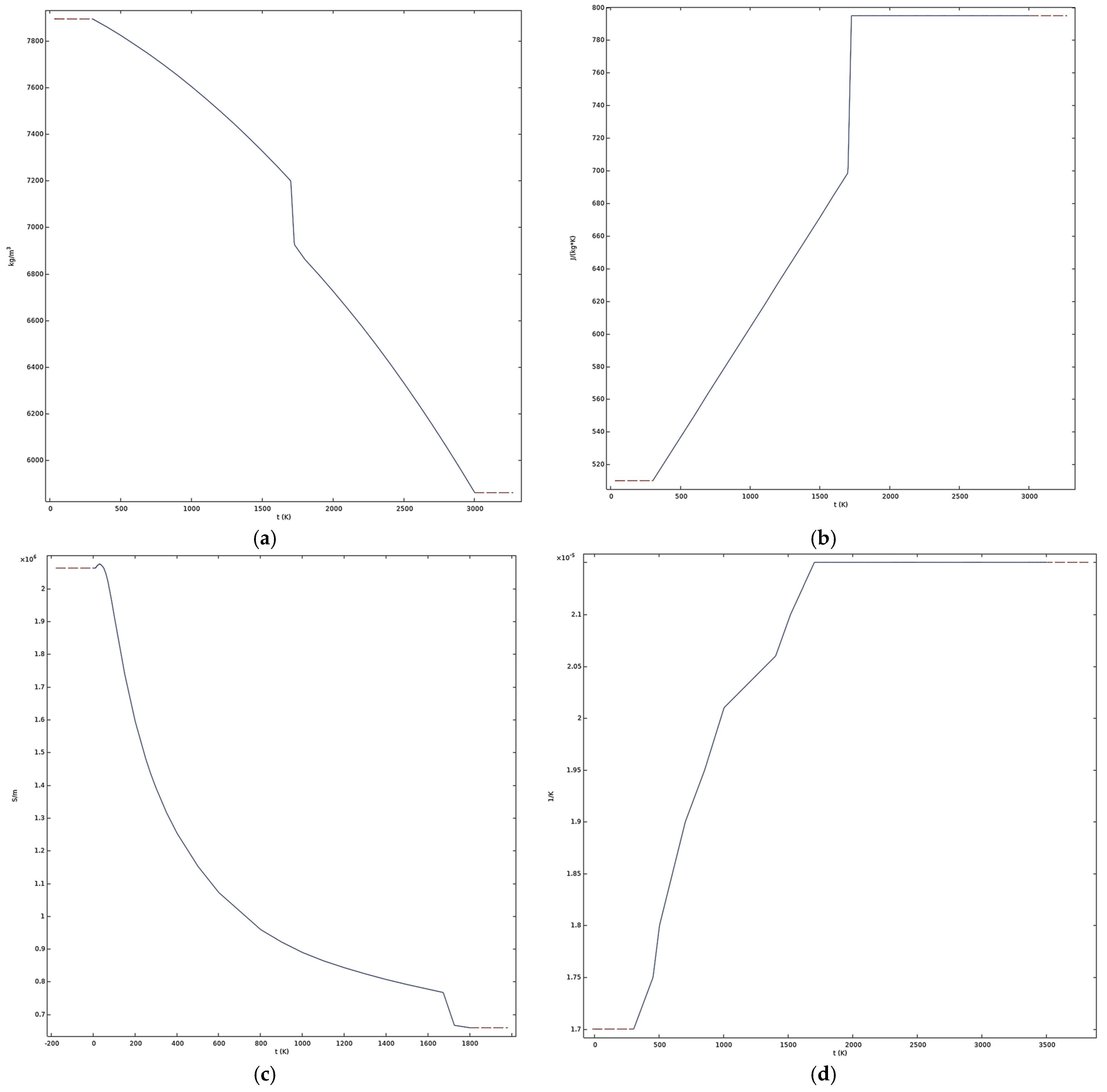
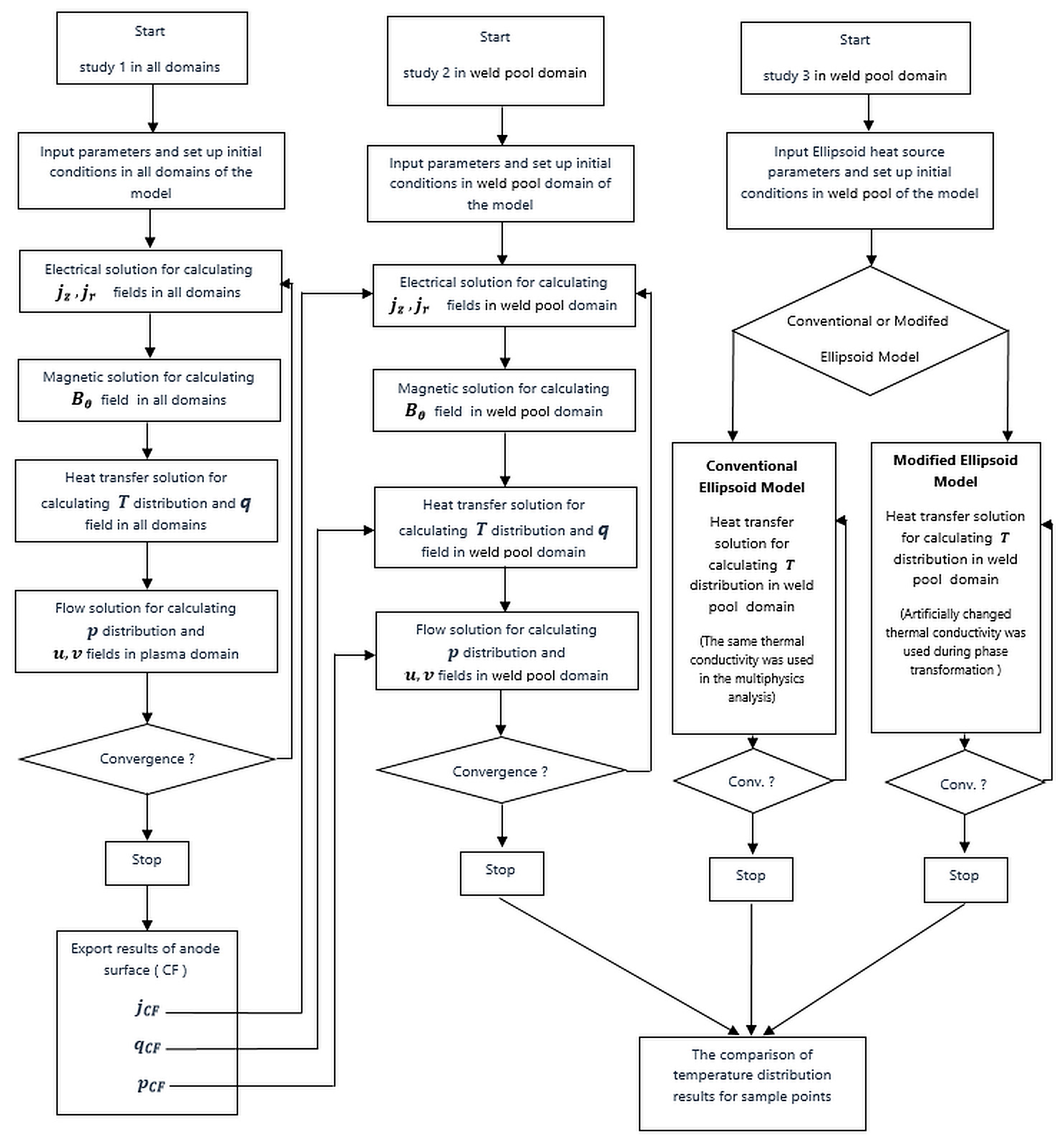
Thus, the resulting velocity and pressure are determined using the previously obtained Lorentz forces and thermal field. If the convergence criteria are not acceptable, all temperature-dependent properties are updated by using the current temperatures, and these steps are repeated until the required convergence is reached. All material properties used in the multiphysics analysis are given in Figure 2, Figure 3 and Figure 4 and Table 4. Detailed COMSOL V5.5 solution procedures are given in Figure 5.

Figure 2.
Some physical properties of the workpiece (anode, 304 SS material); (a) Density of the workpiece; (b) The heat capacity of the workpiece; (c) Electrical conductivity of the workpiece; (d) Thermal expansion coefficient of the workpiece.

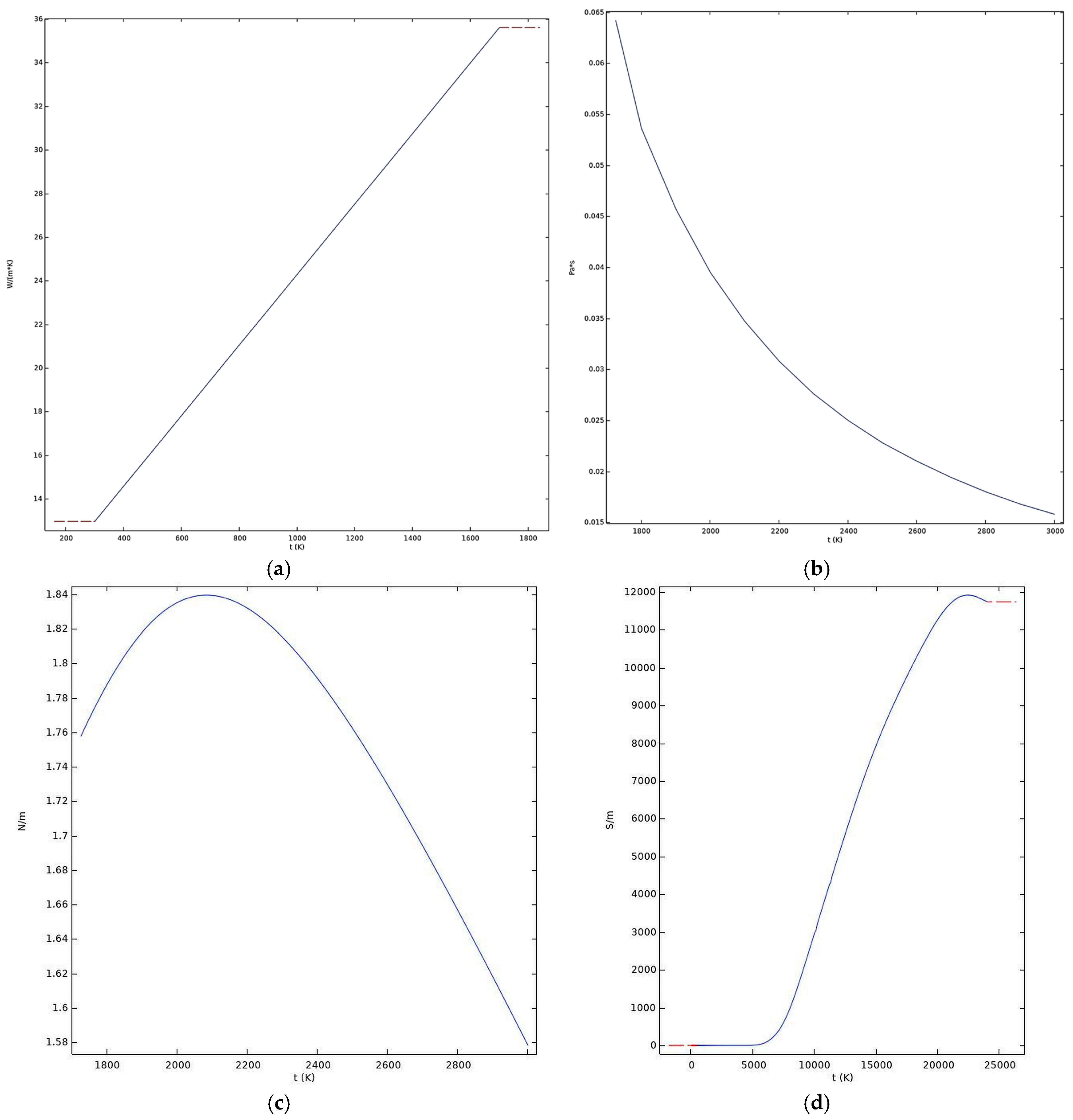
Figure 3.
Some physical properties of the workpiece (304 SS material) and shield gas (Argon); (a) Thermal conductivity of the workpiece (304 SS); (b) Dynamic viscosity of the weld pool (anode, Molten Phase); (c) Surface tension coefficient of the workpiece; (d) Electrical conductivity of the plasma gas (Argon).
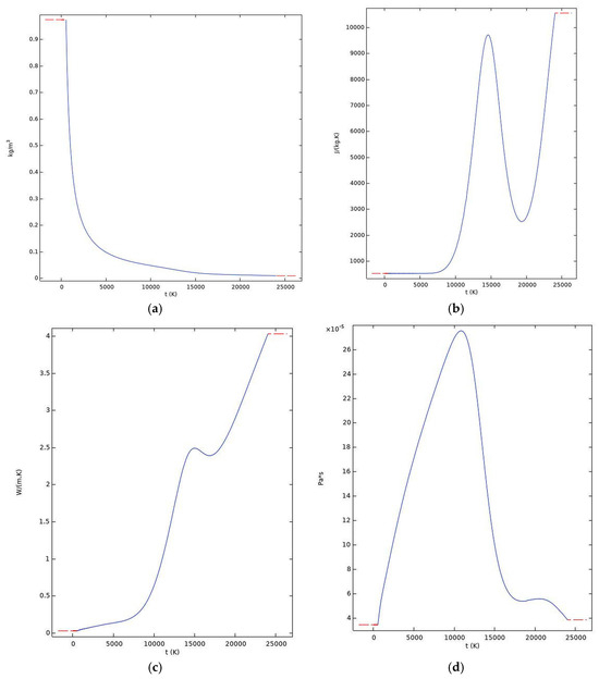
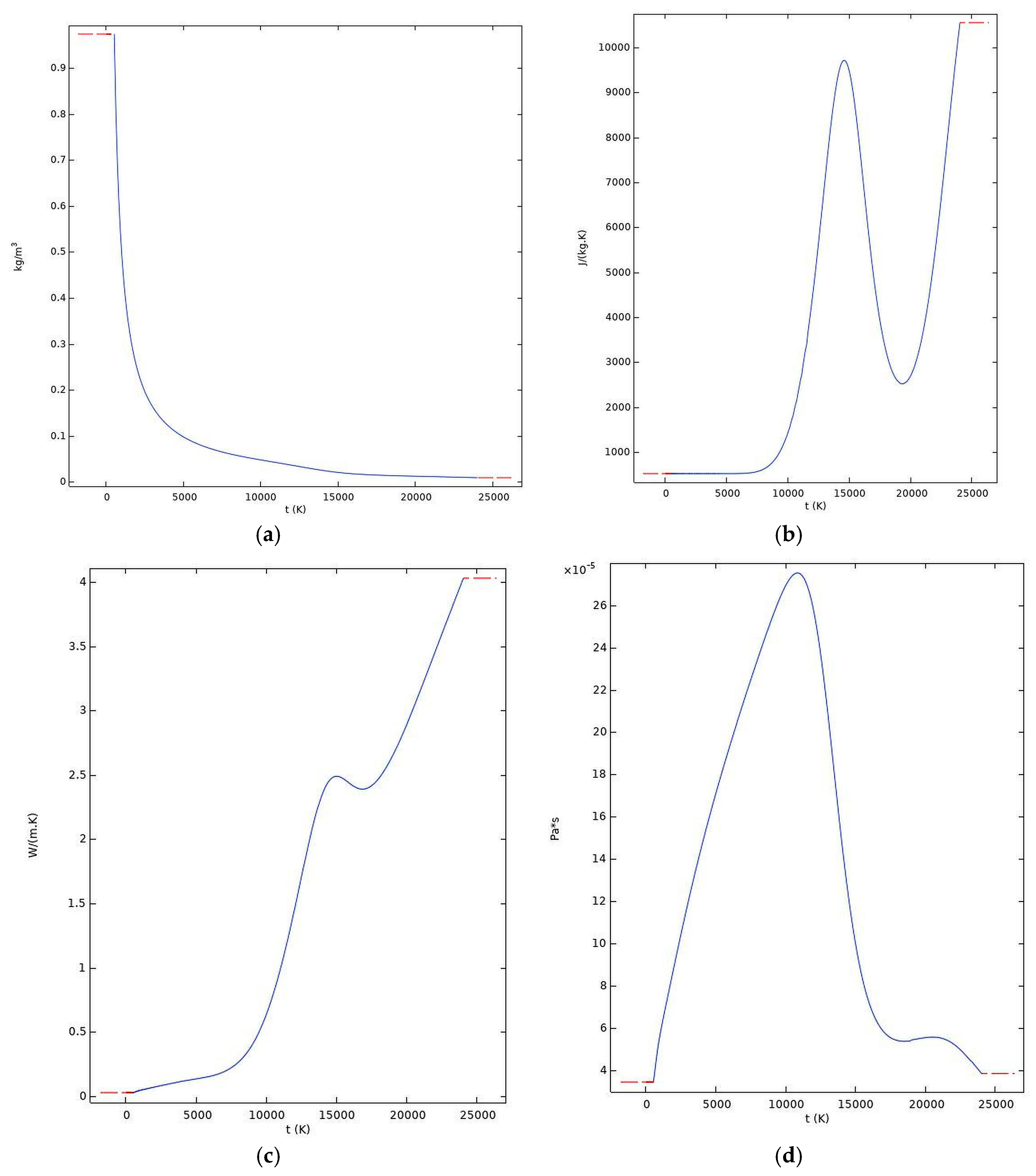
Figure 4.
Some physical properties of the shield gas (Argon); (a) Density of the plasma gas (Argon); (b) Heat capacity of the plasma gas; (c) Thermal conductivity of the plasma gas; (d) Dynamic viscosity of the plasma gas.
Table 4.
Material properties of tungsten cathode.
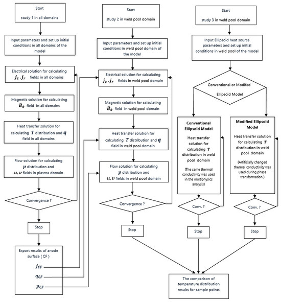
Figure 5.
Flowchart for the multiphysics, conventional, and modified ellipsoid model procedures.
For the ellipsoid heat source model in COMSOL V5.5, the formulas used have a Gaussian distribution form of the power density, as given in Equation (35). In this equation, represents the maximum value of the power density at the center of the ellipsoid. In this heat source modeling, the power is separated into two halves that consist of front and rear quadrants. The power for the two halves is calculated by integration, as in Equation (36).
According to the boundary conditions
the coefficients of heat flux are found as
Finally, the power density distribution inside the front and rear quadrants becomes
Throughout ellipsoid heat source analyses, the parameters are used as follows: I = 150 Amp V = 12 Volt, a = 4.25 mm, and b = 5.40 mm.
Meanwhile, it should be noted that artificially changing the thermal conductivity is a concept that can be implemented in finite element analysis in different ways. Especially in 2D problems (depending on the welding speed), when the torch arrives at the observation section, thermal conductivity is changed to a specific value in the whole area of the FZ. This artificial changing of the thermal conductivity gives good results, as reported in Nart’s work in Ref. [8]. In this research, the problem is modeled in an axisymmetric domain, as the elements in the fusion zone start growing from a point to a certain melted pool size (depending on the parameters used), and all the elements within the melted pool are exposed to artificially increased thermal conductivity. The value of the stirring thermal conductivity is taken at 120 W/m2C, as indicated in Goldak’s work in Ref. [5]. In COMSOL V5.5, this is easily implemented by using phase change calculations in the weld pool region.
In this study, analyses were performed using the COMSOL V5.5 software on a computer equipped with an Intel i7 processor and 32 GB of RAM. The multiphysics model required 37,423 s to complete, whereas the conventional and modified ellipsoid models required approximately 194 s. This indicates a computational efficiency improvement of approximately 193 times in favor of the conventional and modified ellipsoid models compared to the multiphysics analysis.
5. Results and Discussion
All the results obtained during this research can be summarized in three main stages. In the first stage, the arc plasma model is presented. Because the arc plasma inputs are the most important aspects of an arc welding simulation, related results are carefully validated with a well-known reference. In the second stage, the modeling of molten metal flow during GTA welding is fulfilled by implementing well-known formulas for surface tension concerning temperature and sulfur concentration. Then, several points are selected from the melted pool region to obtain multiphysics thermal histories. In the last stage, a comparison of multiphysics, conventional, and modified ellipsoid models is undertaken correspondingly.
5.1. Plasma Model Results and Validation
In the plasma validation process, the COMSOL V5.5 model used in this work is simply modified according to the dimensions and welding parameters taken from Hsu’s research in Ref. [10] (I = 200 A, BC = 10 mm). The obtained results are compared with that of Hsu’s research.
In Figure 6, it can be seen that similar results are obtained even though Hsu et al. assume that on the anode surface (CF), the temperature distribution is taken experimentally, and at the boundary GF, the temperature of 1000 K is postulated.
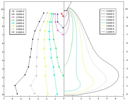
Figure 6.
200 A, 10 mm arc length, argon arc axial temperature distribution, and a comparison with the literature [23].
In Figure 7, the temperature exhibits a rapid increase in front of the cathode due to Ohmic heating, and as the arc spreads (decrease in the current density), the temperature drops to values below 15,000 K close to the anode.
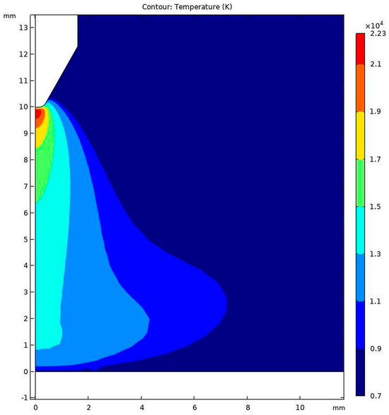
Figure 7.
200 A, 10 mm arc length, and argon arc axial temperature distribution.
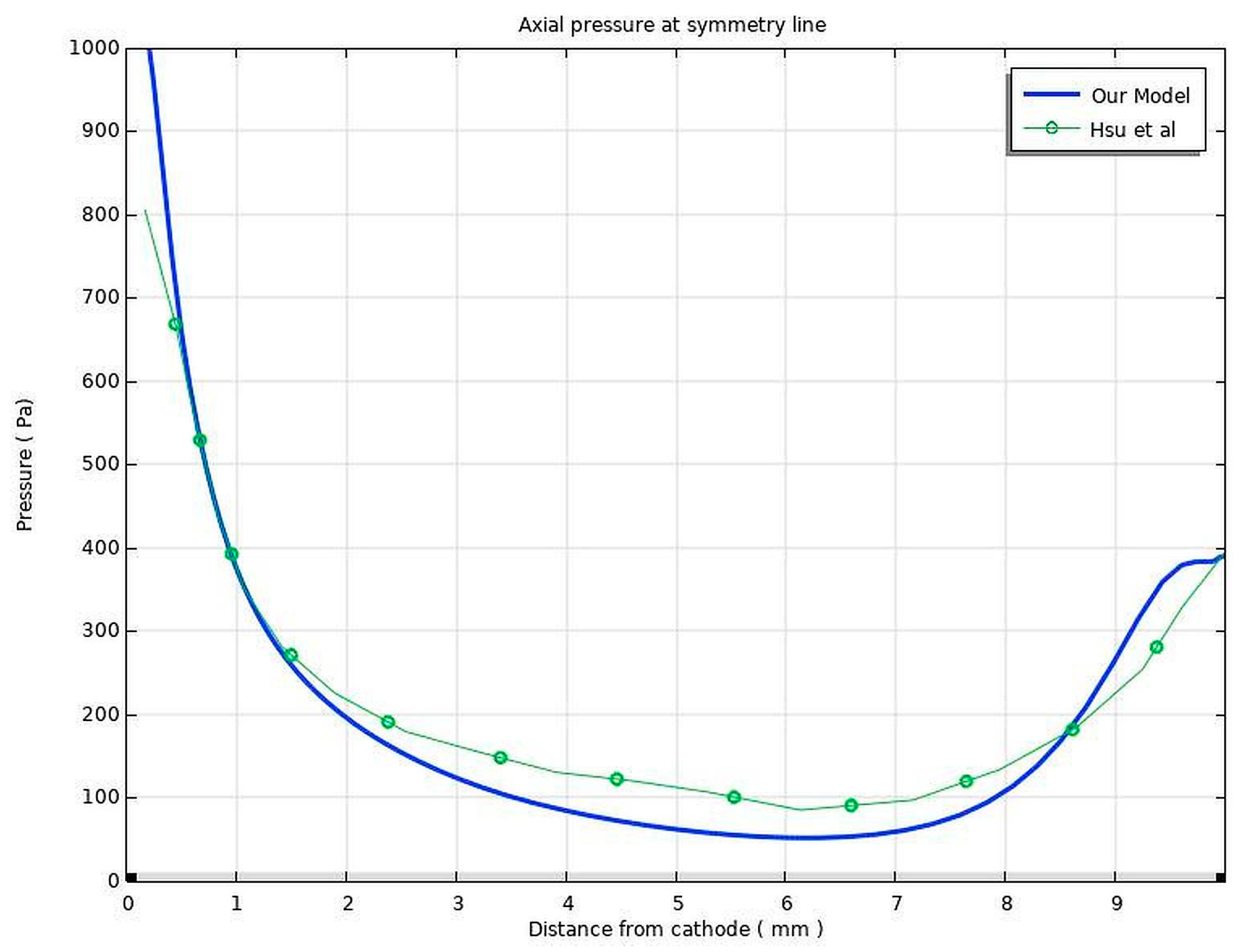
As seen in Figure 8, a large pressure change takes place near the cathode tip because a strong electromagnetic force occurs due to the high current density around. This is because the arc exhibits significant constriction in the vicinity of the cathode tip due to the localized nature of electron emission, which predominantly occurs at a small region on the cathode surface known as the cathode spot. This confined emission zone serves as the principal source of electrons, leading to a highly concentrated current density in that area. As the emitted electrons propagate away from this region, the current distribution expands radially into the surrounding plasma. Consequently, the cross-sectional area of the plasma increases with distance from the cathode, causing a rapid decline in current density despite the conservation of the total current. A strong electric field exists near the cathode, effectively accelerating electrons into the arc plasma. Once within the arc column, these electrons experience frequent collisions with neutral atoms and ions, which diminishes their directional energy while simultaneously contributing to plasma heating. The electron temperature (Te) is significantly elevated near the cathode tip, facilitating enhanced ionization and sustaining electrical conductivity in this region. However, as electrons diffuse outward and approach thermal equilibrium, they decrease, leading to a reduction in conductivity and a further decline in current density in the outer regions of the plasma [29].
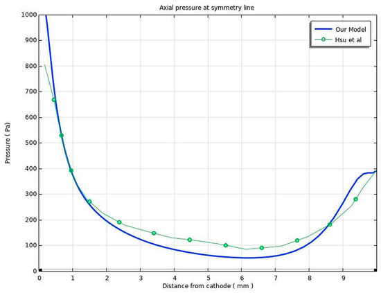
Figure 8.
200 A, 10 mm arc length, argon arc axial pressure, and a comparison with the literature [10].
This behavior is primarily attributed to the increase in arc power with higher current levels, which leads to a corresponding expansion in both the current density within the arc column and the effective conductive cross-sectional radius. As the arc radius expands, the spatial extent of the pressure distribution within the arc also increases. Furthermore, the electromagnetic force—serving as the primary driver of arc plasma fluid flow—intensifies with rising current density. Consequently, an increase in current density is expected to enhance the electromagnetic force, thereby contributing to a rise in the maximum arc pressure [30]. Additionally, when the pressure effect vertically reaches the surface of the workpiece (anode), there is an increase in pressure because of the gas–wall impact effect.
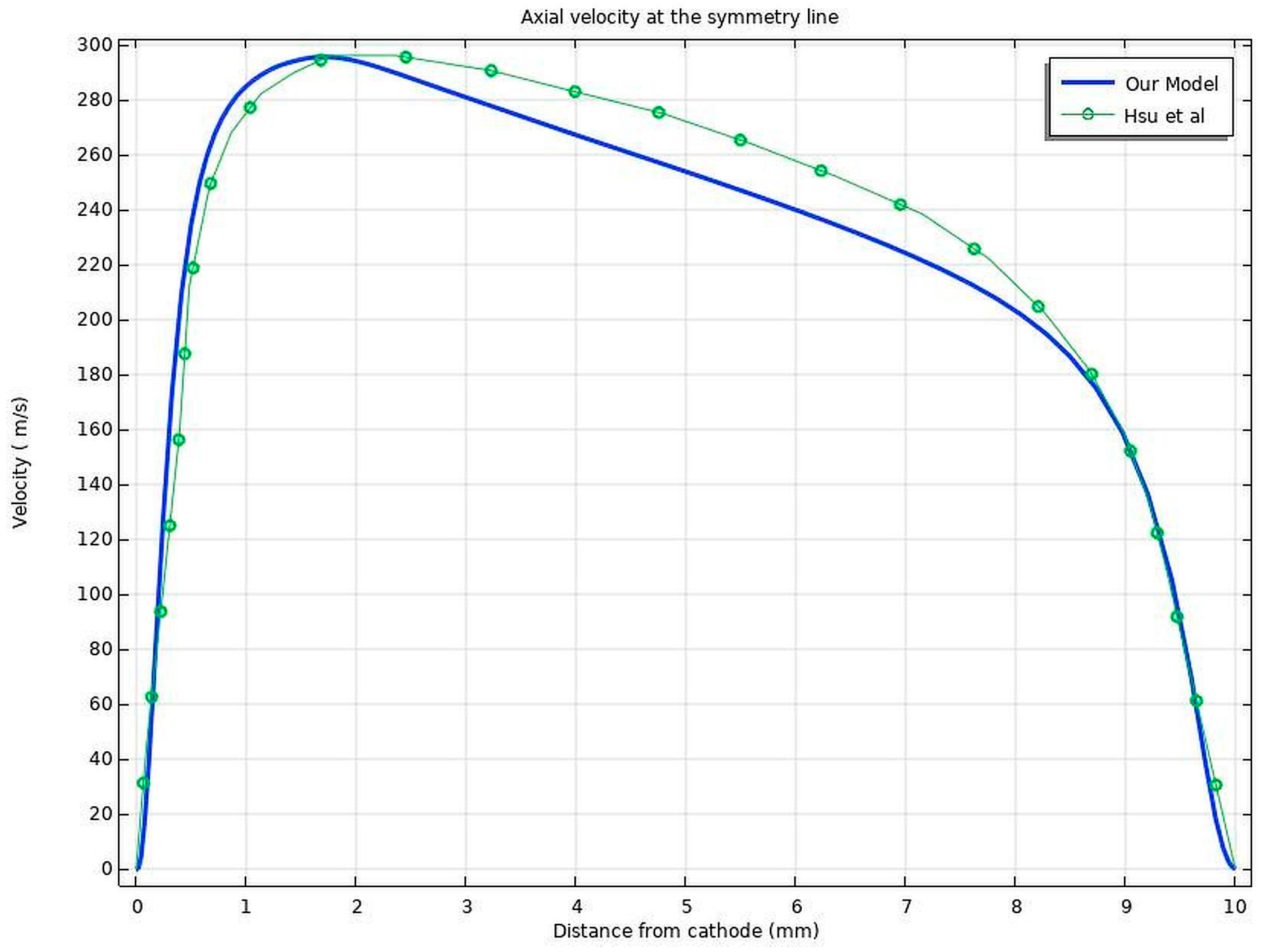
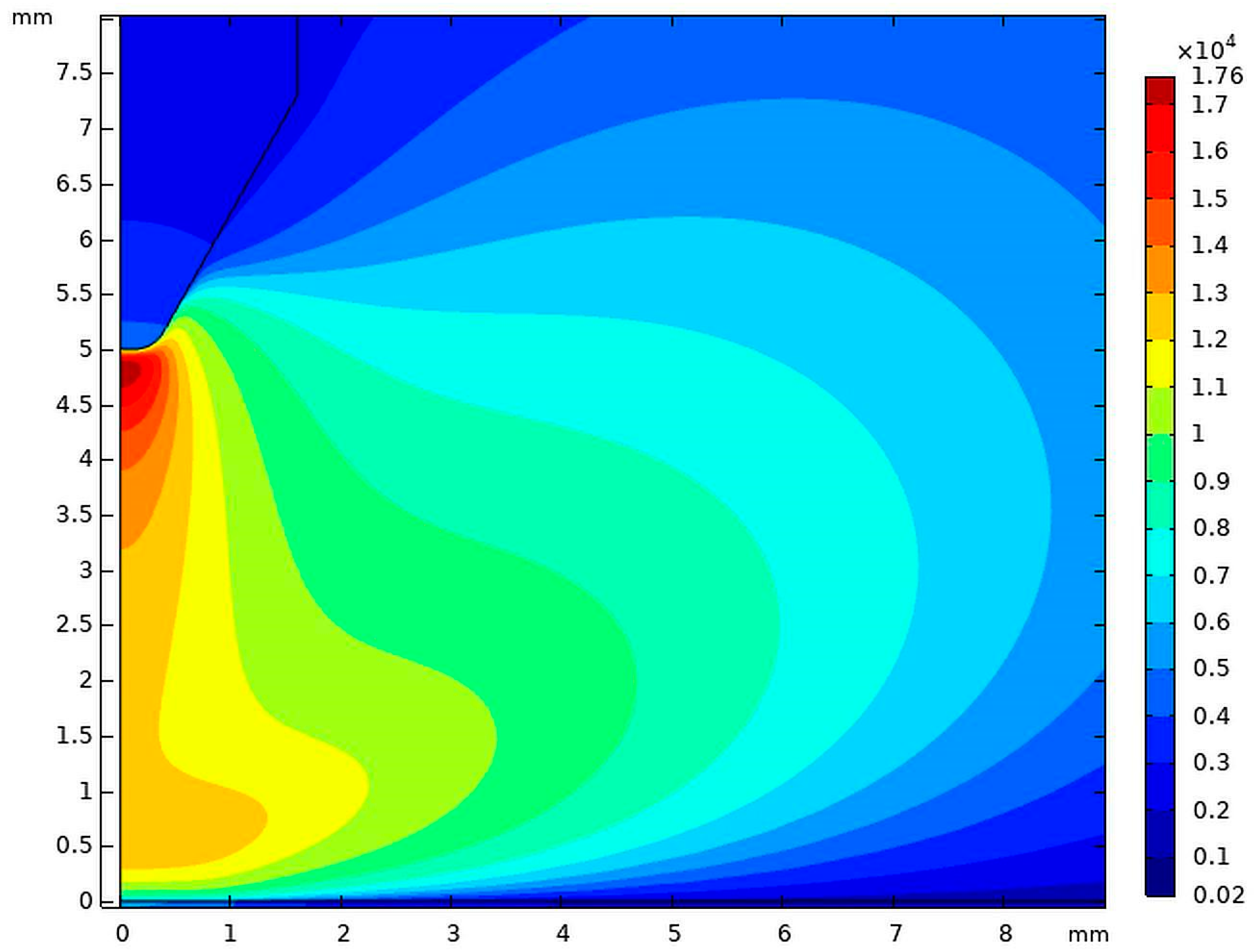
In Figure 9, the axial velocity rises to a maximum at the electrode tip due to the strong pressure difference; the axial velocity decreases rapidly as approaches the workpiece and becomes zero. In Figure 10, the contour plot of the velocity distribution is shown.
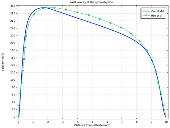
Figure 9.
200 A, 10 mm arc length, argon arc axial velocities, and a comparison with [10].
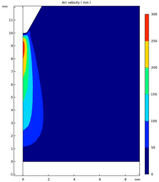
Figure 10.
200 A, 10 mm arc length, and argon arc axial velocity distribution.
5.2. Weld Pool Results and Validation
The multiphysics model results need validation to go further in this research. To validate the multiphysics solution procedure developed in this research, the research by Tanaka et al. [25] is selected. In Tanaka’s study, the authors give calculations of the time-dependent two-dimensional asymmetrical distributions of temperature and velocity in a whole region of the welding process.
Accordingly, the authors also provide experimental results in their paper. Therefore, the same model with the same boundaries, definitions, and parameters is constructed in COMSOL V5.5 software for validation, and corresponding results are obtained.
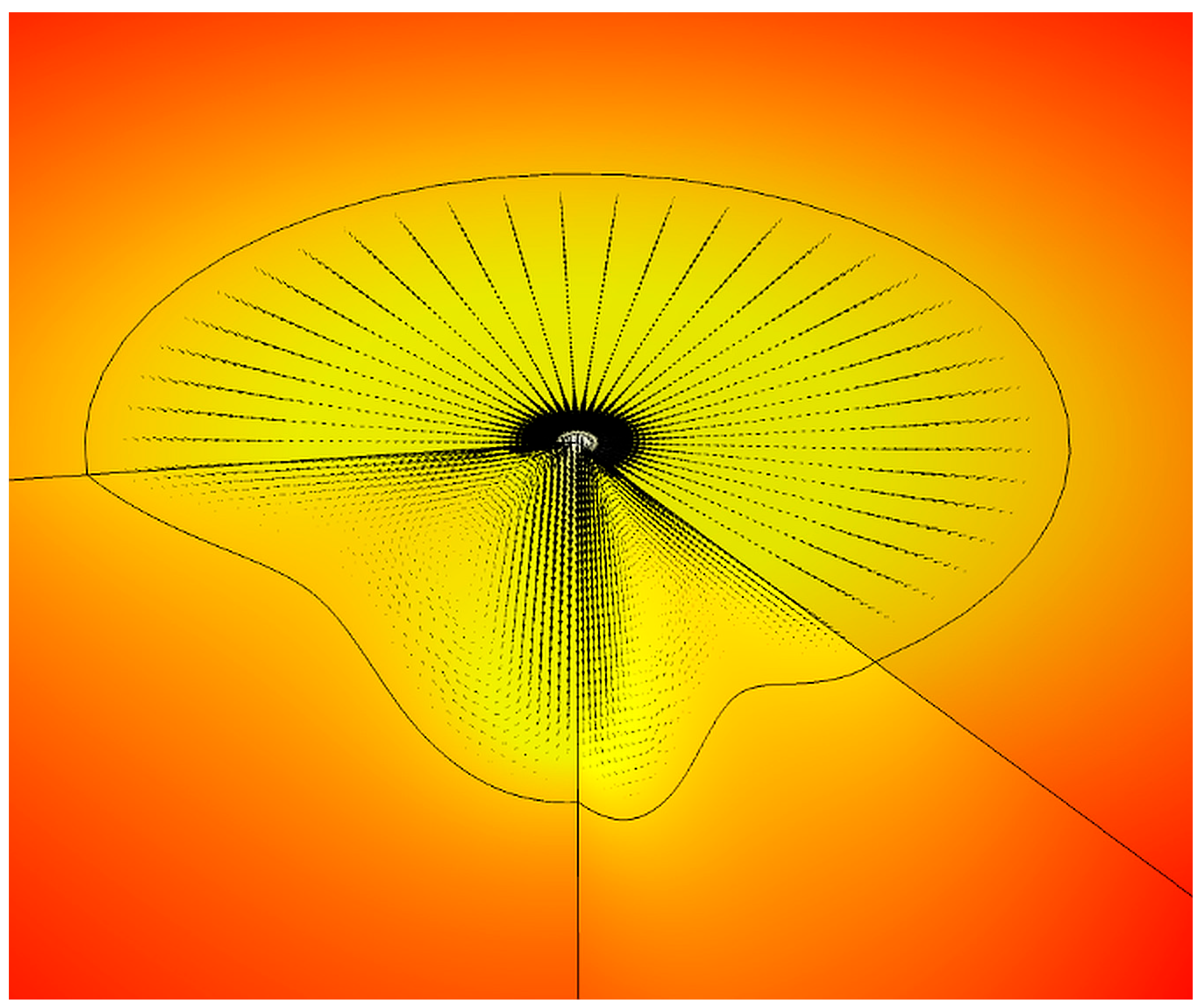
In Figure 11, it can be seen that electric arc plasma formation is obtained from the corresponding COMSOL V5.5 model. If the related results are used as input in the modeling of molten metal flow in the GTA welding process, the weld pool problem is solved and a corresponding temperature and melted metal flow solutions are obtained. According to the results achieved, it is observed that a liquid with a high surface tension makes the surrounding liquid with a low surface tension move strongly. Expectedly, Marangoni convection dominates the fluid flow in the weld pool due to the temperature gradient of surface tension.

Figure 11.
Temperature distribution in weld pool region (150 A, 5 mm arc length).
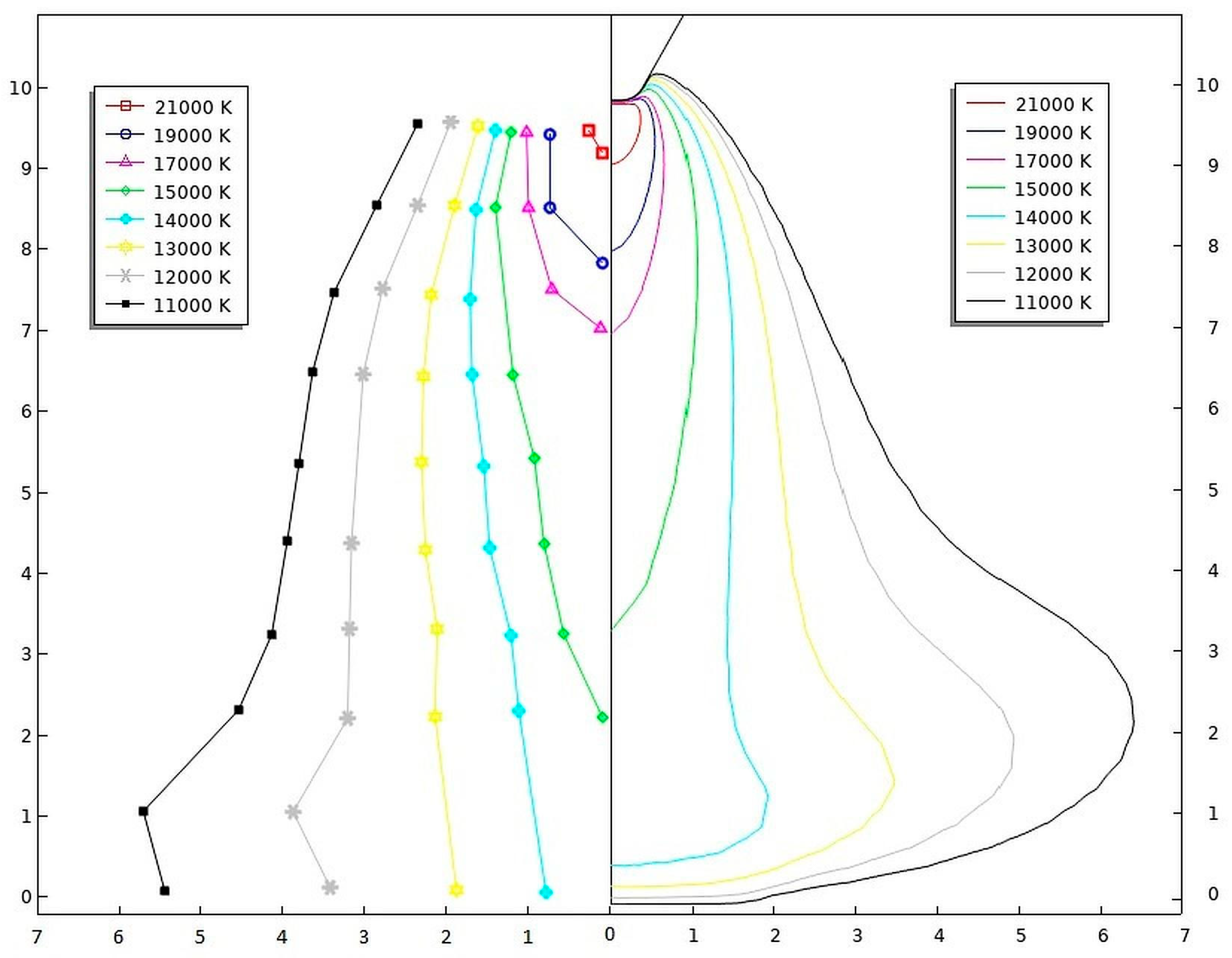
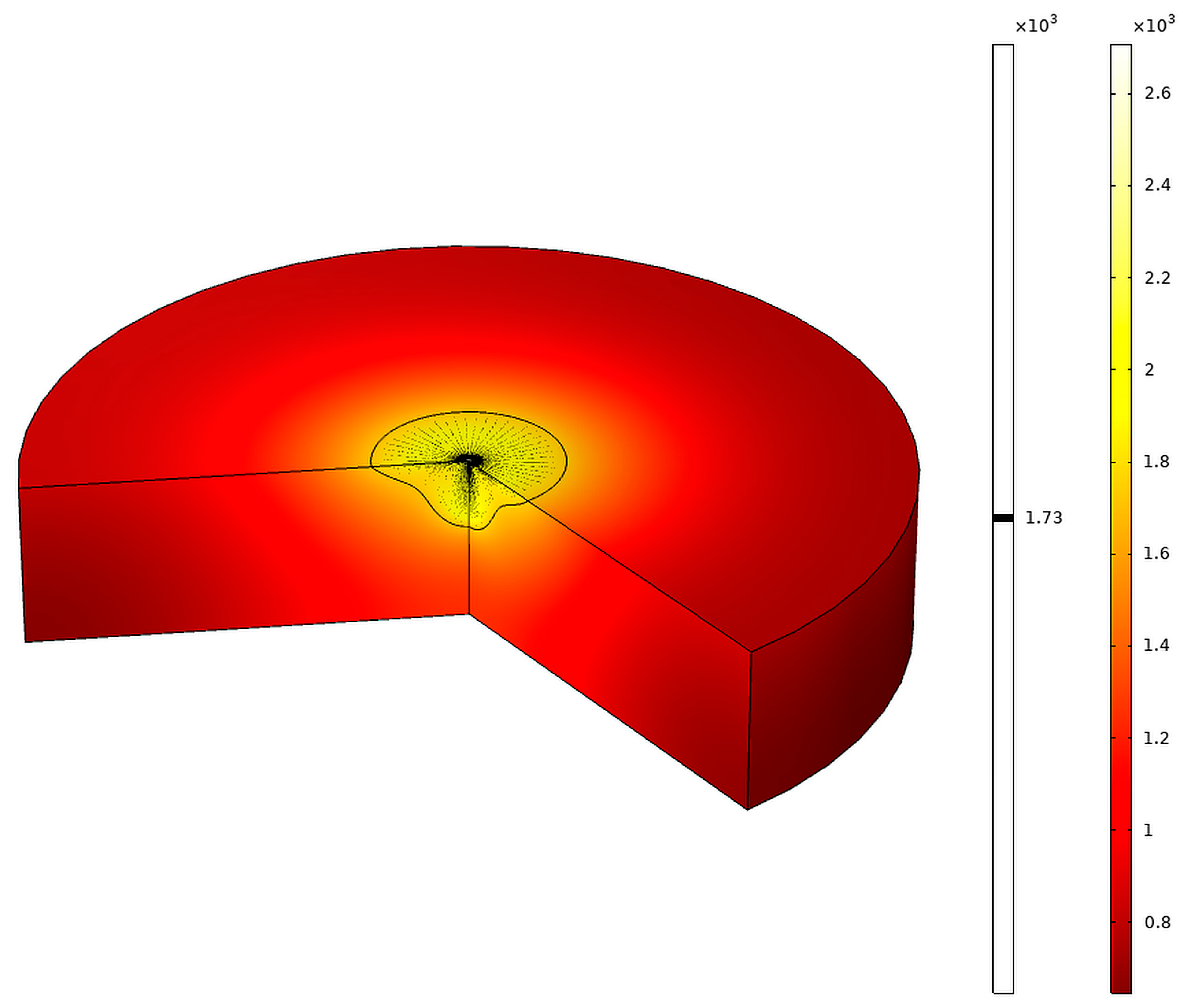
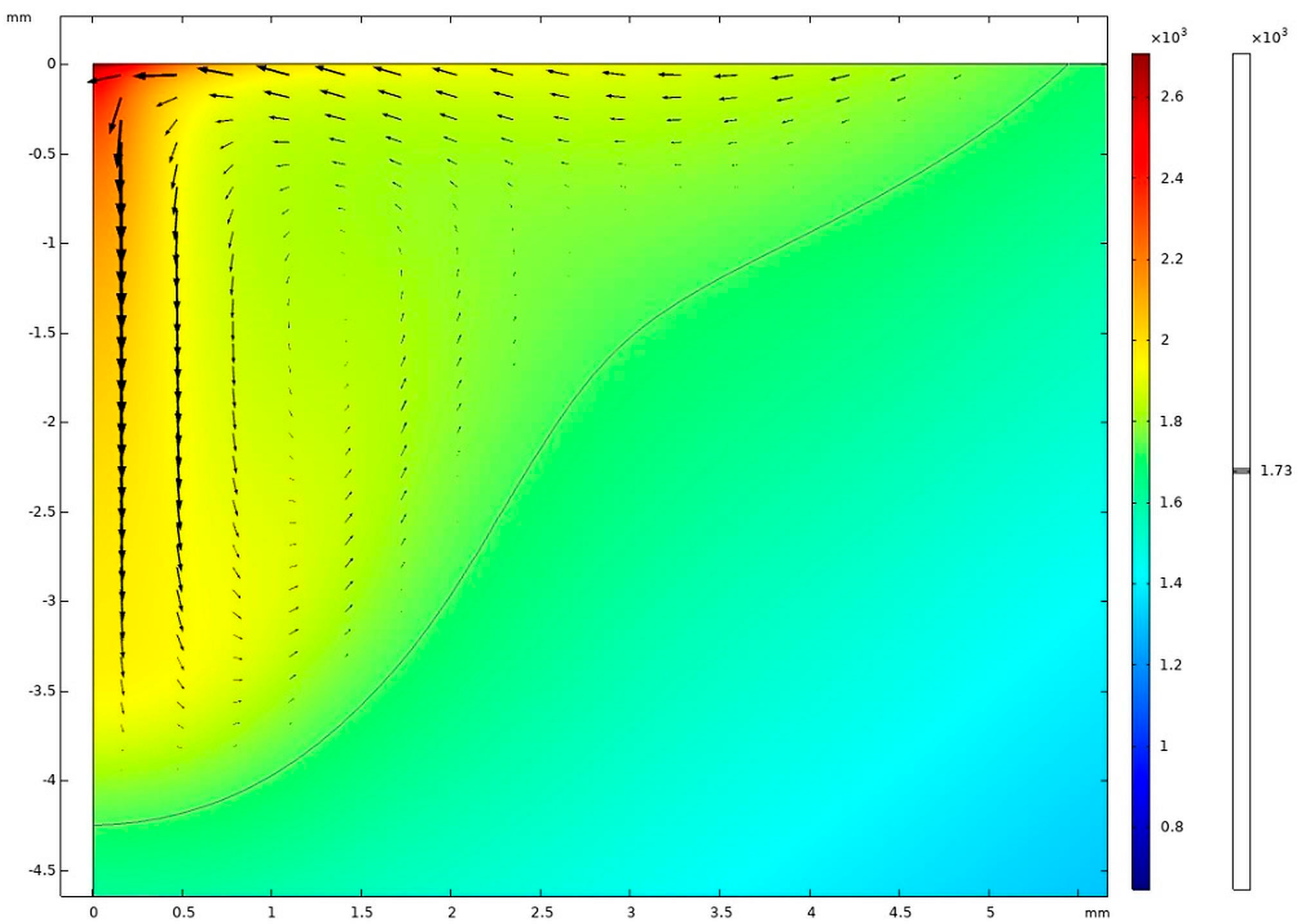
In Figure 12 and Figure 13, the temperature and velocity distribution in the weld pool region can be seen in the 3D view of axisymmetric results. Accordingly, if the results in the welding region appear in cross-sectional views, at the right part of the weld cross-section in Figure 14 and Figure 15, two vortices can be seen in the weld pool; the first is a counterclockwise vortex near the center of the weld pool, forming an inward fluid flow at the surface, and the second is clockwise vortex near the edges of the weld pool, forming an outward fluid flow. It can be seen that the first counterclockwise vortex is visibly leading and forms a deep and narrow weld pool. However, the second clockwise vortex induces a wide and shallow weld pool.

Figure 12.
Temperature and velocity distribution in the weld pool region in 3D (150 A, 20 s, 5 mm arc length).
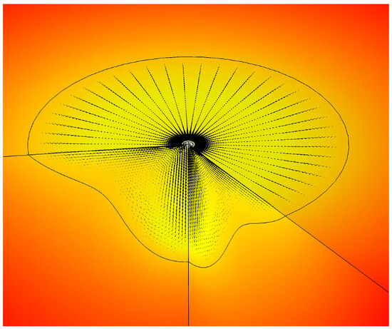
Figure 13.
The zoom view of temperature and velocity distribution in the weld pool region in 3D (150 A, 20 s, 5 mm arc length).
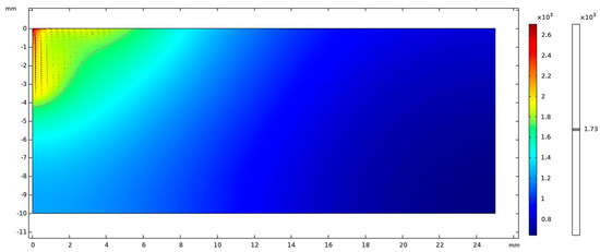
Figure 14.
Temperature and velocity distribution in the weld pool region (150 A, 20 s, 5 mm arc length).
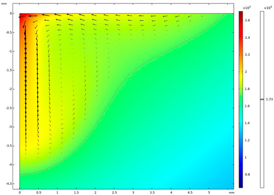
Figure 15.
Zoom view of temperature and velocity distribution in the weld pool region (150 A, 20 s, 5 mm arc length).
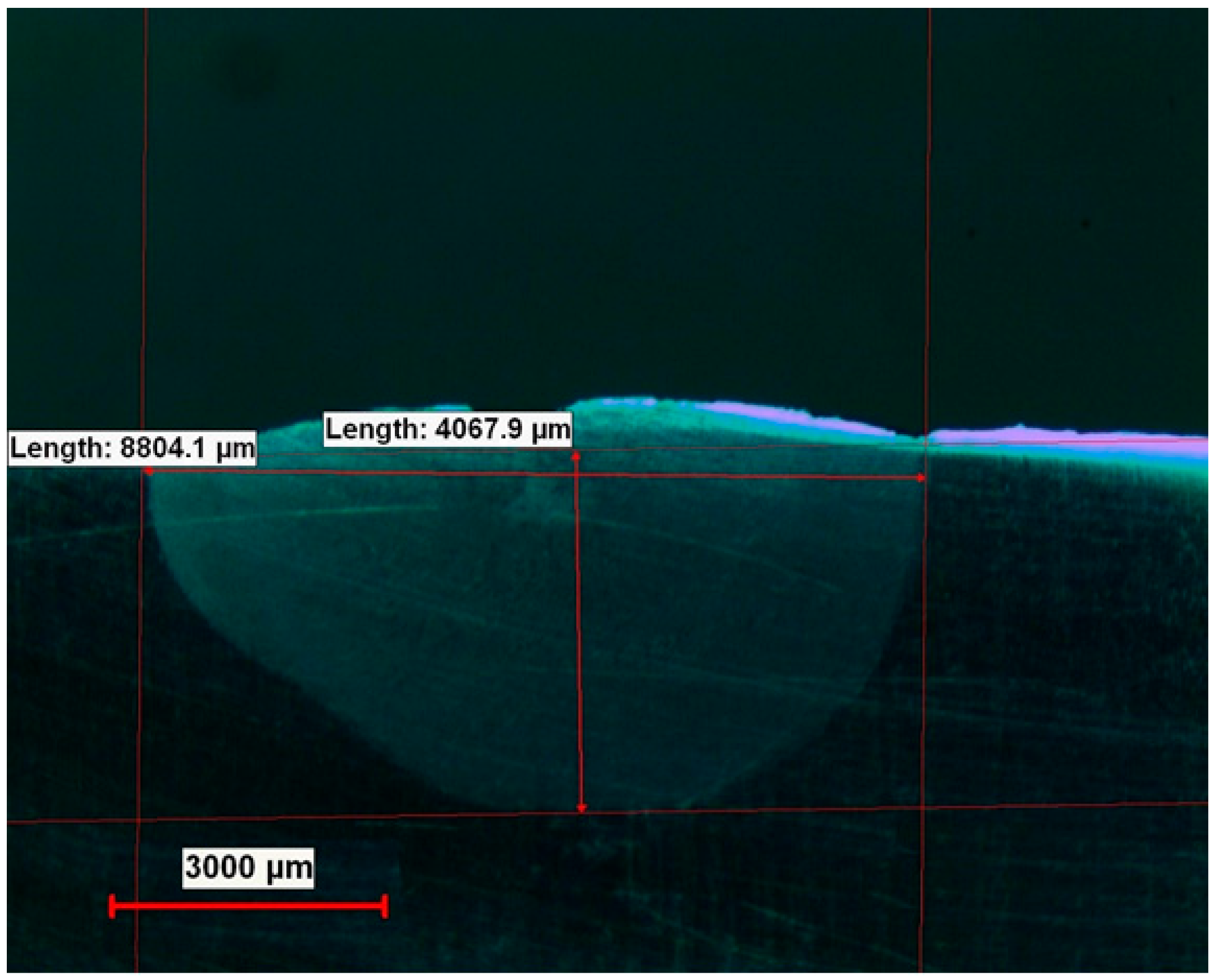
In the validation part of this research, it is clear in Table 5 that the COMSOL V5.5 model used in our study gives similar results to those of Tanaka et al. Both simulations are extremely close to the experimental result presented in Ref. [25]. Additionally, the authors also performed an experiment to validate Tanaka’s results using the same welding parameters. As shown in Figure 16, at least, the pool sizes are found to be almost close to Tanaka’s results.
Table 5.
Experimental weld pool dimensions and a comparison with the literature [25].
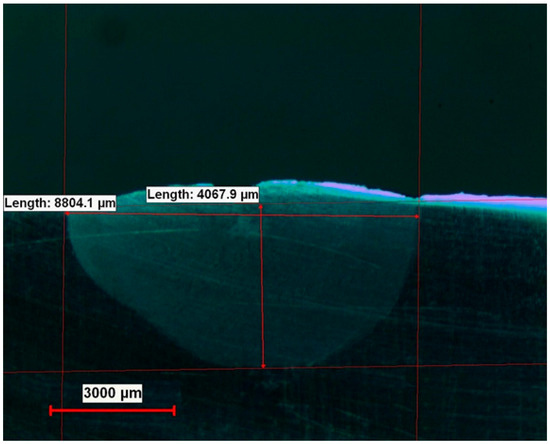
Figure 16.
Experimental results (150 A, 20 s, 5 mm arc length).
5.3. Comparison of Multiphysics, Conventional, and Modified Ellipsoid Models
After a multiphysics TIG welding model in the COMSOL V5.5 environment is developed and a specific TIG welding analysis is performed to obtain all the necessary physical information in a welding pool, it is essential to identify the similarities and differences between the multiphysics and approximate models. In the literature, it is well known that the double-ellipsoidal heat source model (classical and modified forms) is a practical approach and is easy to use for the finite element method [5,6,7,8].
Therefore, the double-ellipsoid model is extensively studied for temperature distribution during the arc welding process in engineering applications.
Nart et al. [8] show that the accuracy of finite element welding simulations using a double-ellipsoid approximate heat source model can be improved by increasing conductivity in 2D. This is true not only for particular nodes that are exceeding the melting temperature, as suggested in [8], but also for all nodes in the welding pool region when the torch reaches the right-observation point to simulate the convective stirring effect (modified double-ellipsoid method) in the welding pool. By doing so, irregular weld bead shapes can be analyzed by using a double-ellipsoid heat source model without any difficulty.
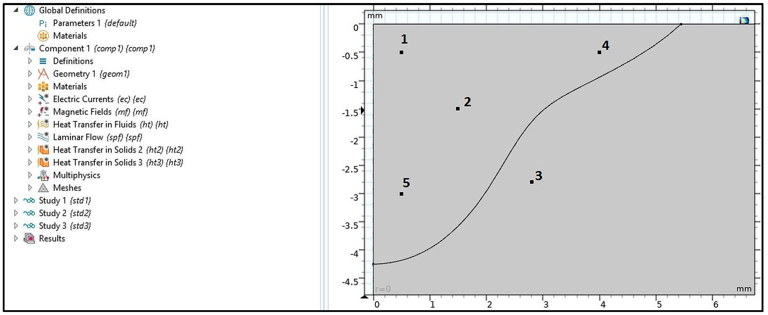
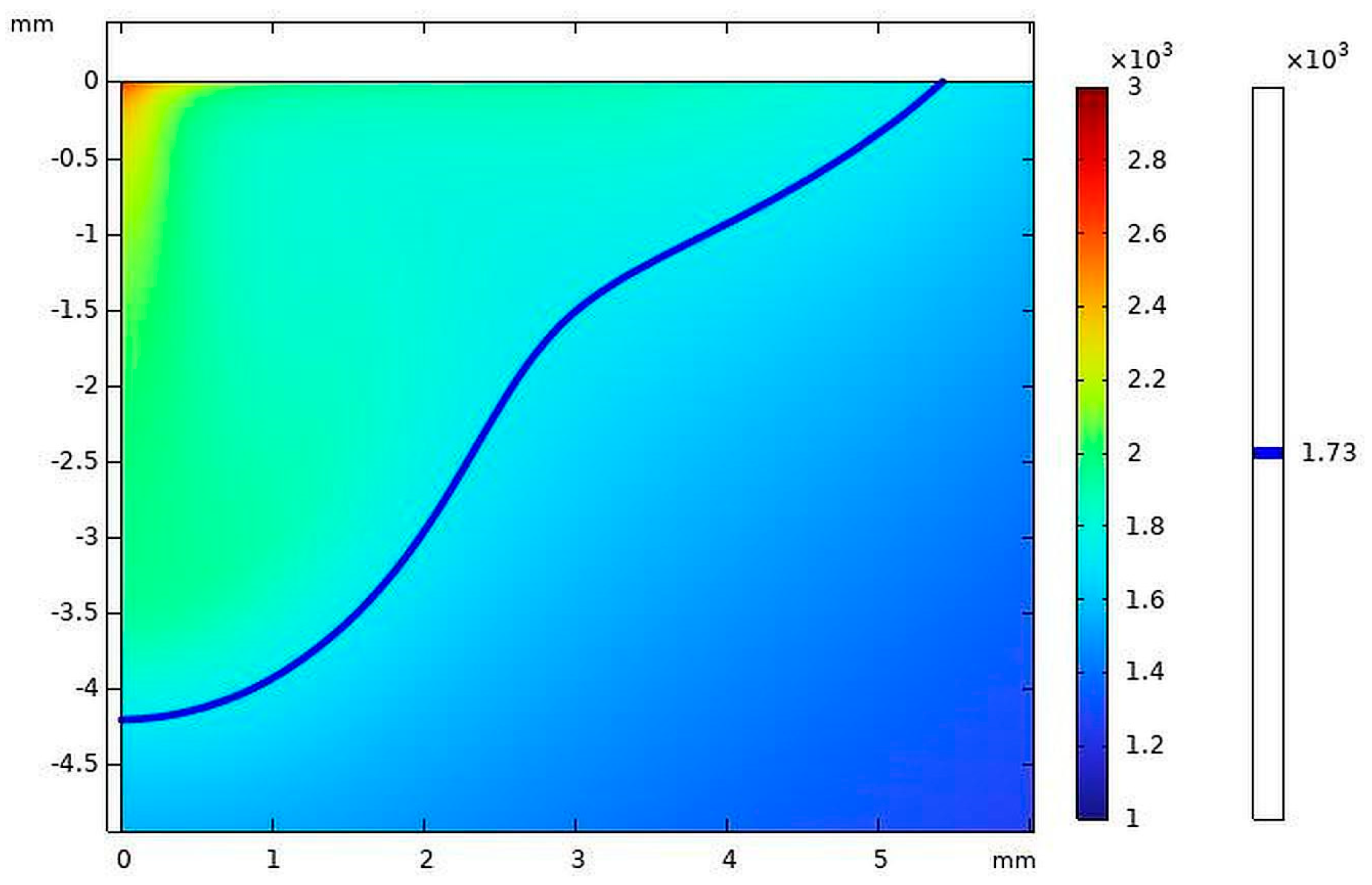
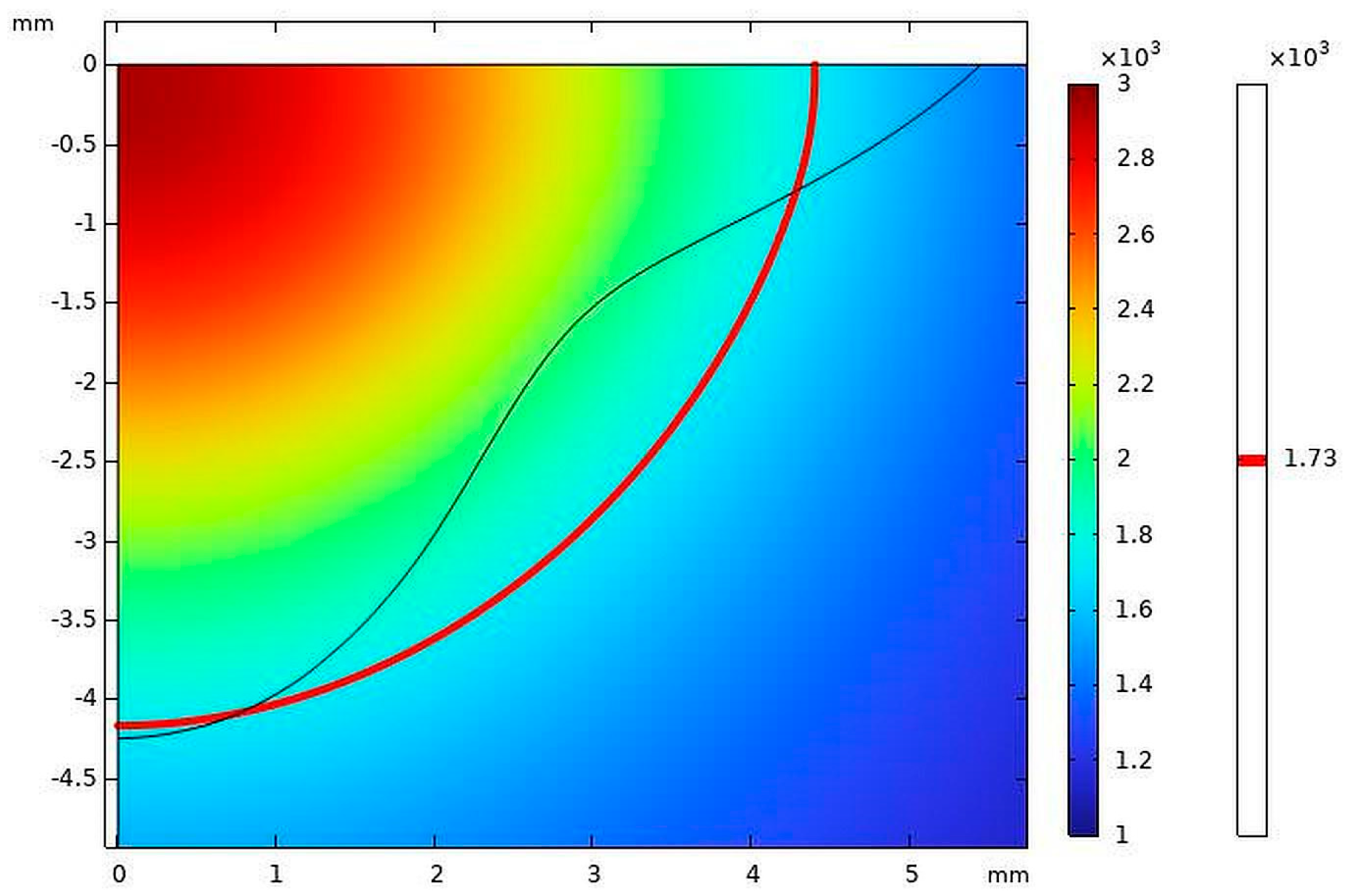
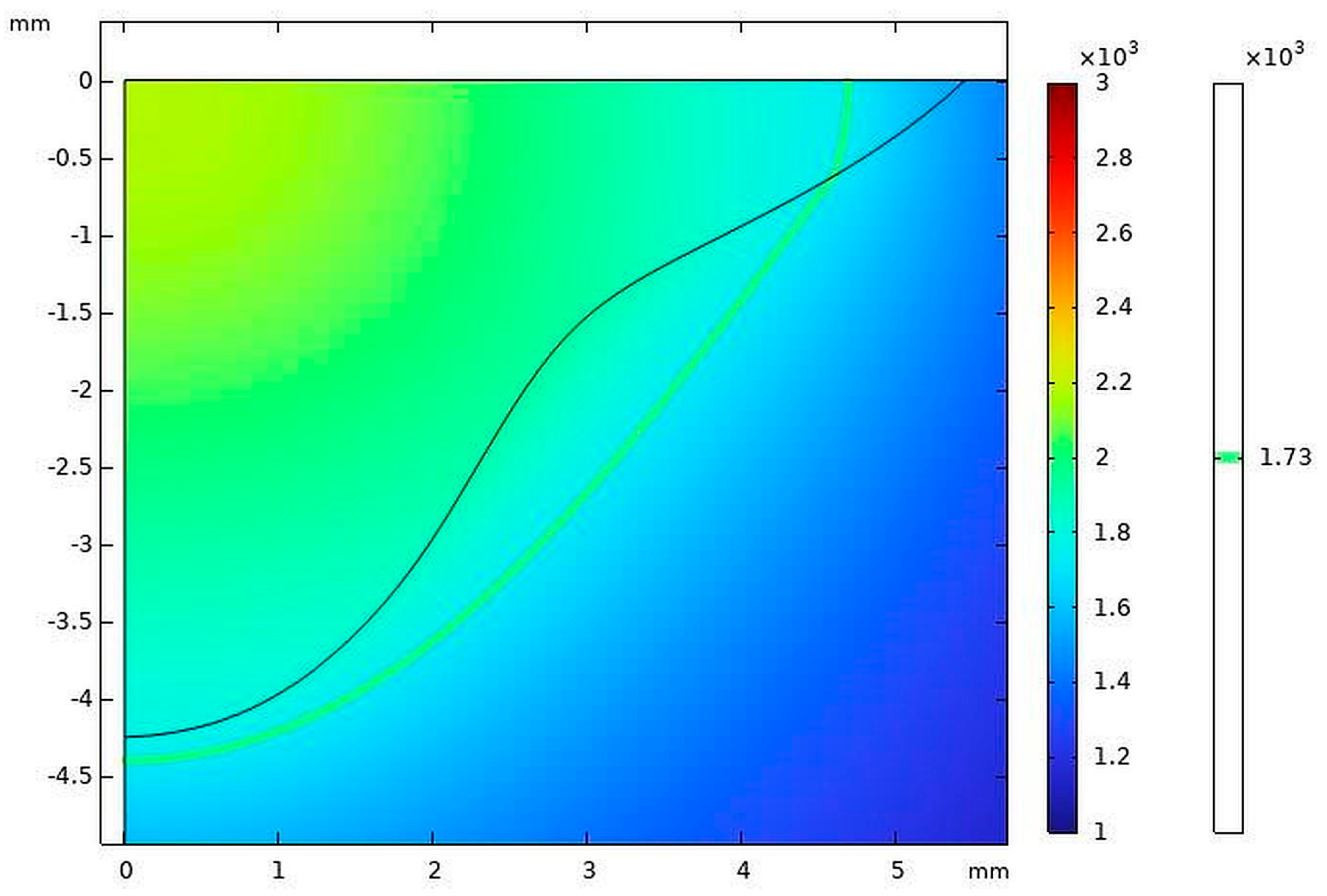
Although the modification of double-ellipsoid heat source application in 2D works as shown in [8], this intuitive approach needs to be verified using multiphysics modeling in the COMSOL V5.5 environment. To do this, a new model in the COMSOL V5.5 software environment, as shown in Figure 17, is prepared for an approximated ellipsoidal heat source using the same welding parameters, geometry, and boundaries as used in the COMSOL V5.5 multiphysics model. Additionally, Figure 18, Figure 19 and Figure 20 show the multiphysics, conventional, and modified ellipsoidal model solutions for the weld pool formation. The blue, red, and green curves in the figures show the borders between the FZ and HAZ.
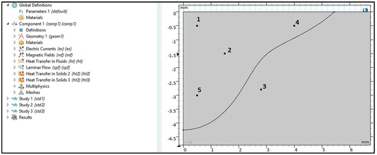
Figure 17.
Model and sampling points for comparing the multiphysics and modified ellipsoidal models.

Figure 18.
Multiphysics weld pool region at 20 s.
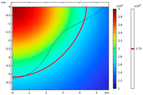
Figure 19.
Ellipsoidal weld pool regions at 20 s.

Figure 20.
Modified ellipsoidal weld pool regions at 20 s.
Therefore, to compare the results of these different welding models, for each model, five different locations are selected and defined as shown in Figure 17.
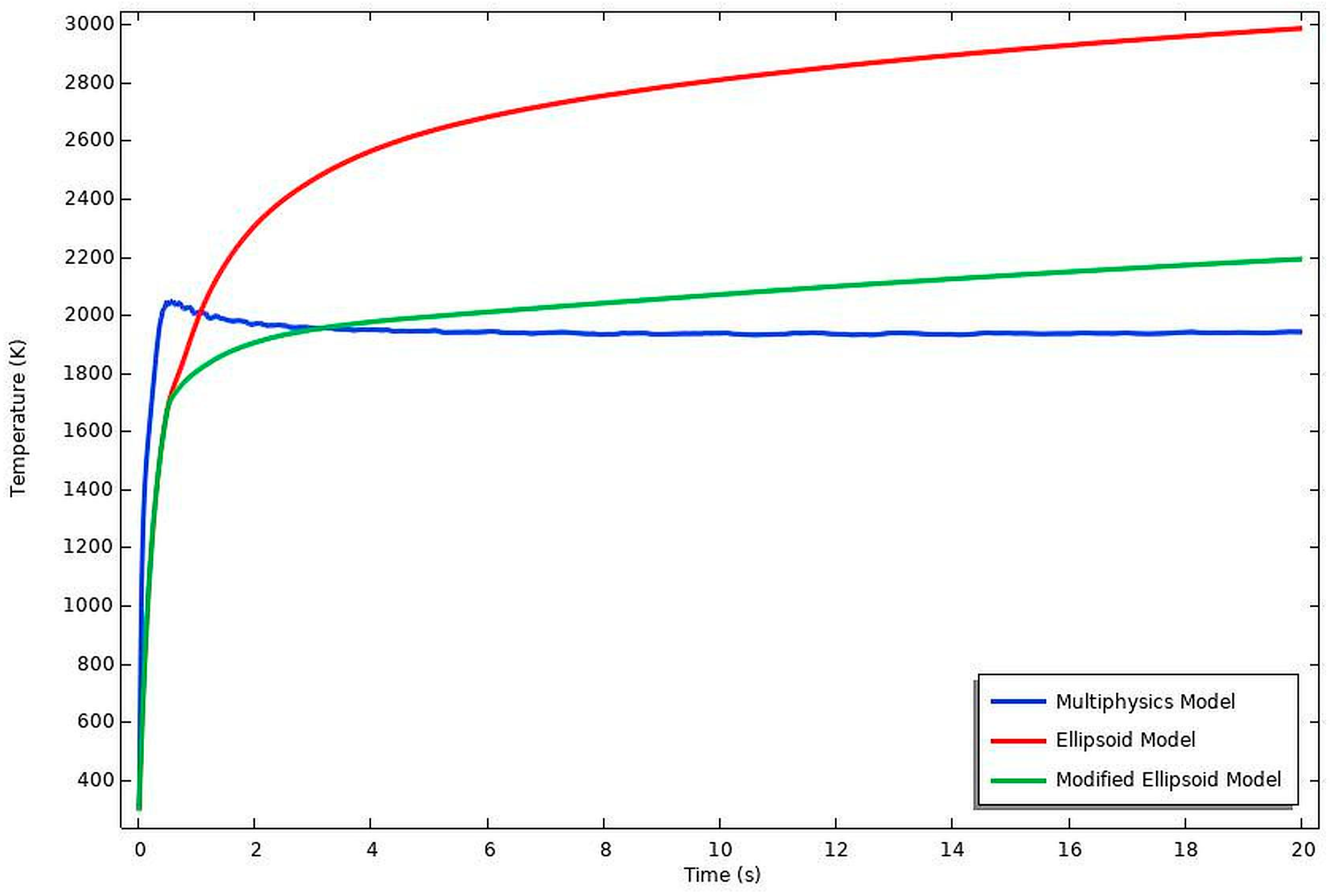
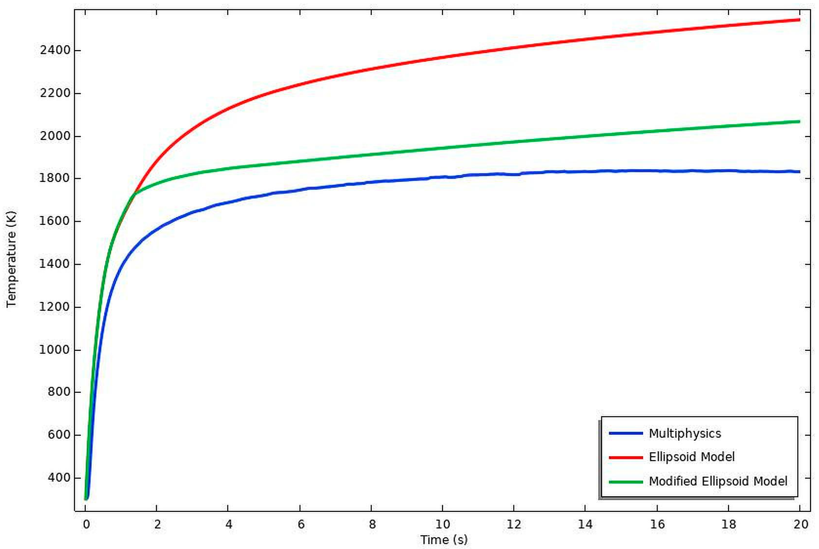
Four of them are located inside the weld pool region. Additionally, the last one is selected to be in the heat-affected zone. If the temperature histories of all the corresponding points are compared, good results are obtained. Especially, for the observation locations at points 1 and 2, the application of the modified double-ellipsoid method significantly generates a closer temperature history than that of the conventional ellipsoidal method, as shown in Figure 21 and Figure 22.

Figure 21.
Temperature history for point 1.
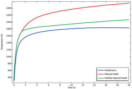
Figure 22.
Temperature history for point 2.
In particular, this situation is highly important in the middle part of the fusion zone. A good approximation of the temperature history in this region affects the acceptable residual stress calculations. Moreover, this improved accuracy in predictions at the low cost of computer power opens a new way for more reliable simulations of welding in various welding problems, such as hot cracking that takes place in the fusion zone (FZ) at high temperatures.
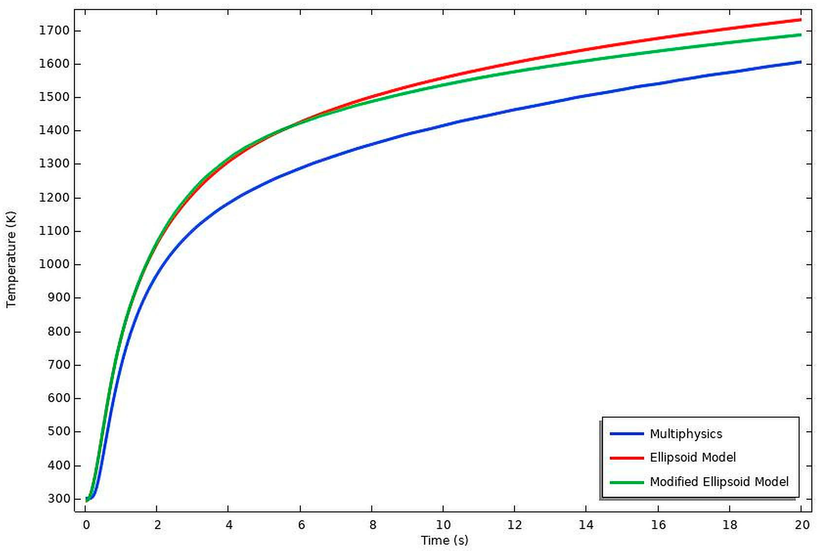
Similarly, at point 3 in the heat-effected zone (HAZ), the ellipsoidal methods give a similar temperature history until the metal melts, as shown in Figure 23. However, after the melting, the modified ellipsoidal method gets slowly closer to the multiphysics solution. Furthermore, for point 4, both ellipsoidal methods also give similar temperature histories, as shown in Figure 24. The modified ellipsoidal method gets closer to the multiphysics solution as time increases. Finally, in point 5, the temperature histories between the multiphysics and modified ellipsoidal methods develop a good agreement. Correspondingly, the temperature differences become gradually closer to each other as the stirring effect becomes dominant in the vertical direction, as seen in Figure 25.
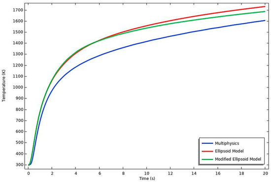
Figure 23.
Temperature history for point 3.
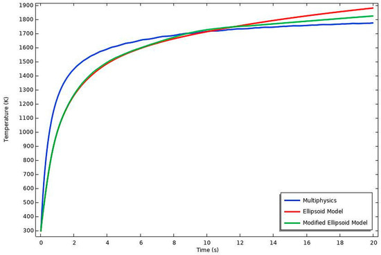
Figure 24.
Temperature history for point 4.
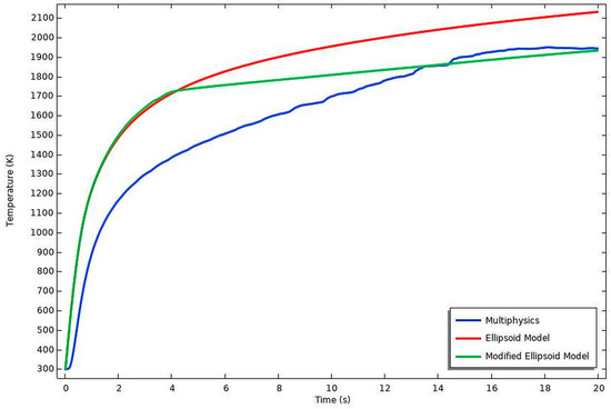
Figure 25.
Temperature history for point 5.
The findings of this research offer important information on future perspectives and industrial applications. In the context of thermal modeling for welding and additive manufacturing processes, accurate representation of heat transfer and material behavior remains critical for predicting structural integrity and performance. This work explores the practical applications of a modified ellipsoidal heat source model across various domains, emphasizing its advantages over conventional formulations. In arc welding, the stirring of the molten pool is predominantly driven by electromagnetic forces, whereas in laser welding, buoyancy effects induced by high-intensity heat input can significantly influence fluid flow. The modified thermal conductivity method, when integrated with the ellipsoidal heat source model, enhances simulation fidelity under such conditions and proves especially effective in hybrid laser-arc welding and parameter-sensitive additive manufacturing.
In advanced manufacturing systems, where automation plays a central role, sensor integration becomes essential. Vision systems are widely utilized to track weld bead geometry and torch alignment; however, accurate penetration measurement remains a technical challenge. Plasma Charge Sensors (PCS), as demonstrated by Li et al. [31], offer a viable solution by correlating the penetration depth with average voltage readings. Incorporating data from PCS and vision sensors into AI-driven frameworks enables real-time refinement of heat source parameters, paving the way for intelligent control in robotic welding systems.
Beyond real-time process monitoring, the modified model significantly improves thermal distribution estimates within the fusion zone (FZ), offering greater precision in residual stress calculations. This enhancement is particularly relevant for assessing post-weld mechanical behavior, including crack initiation and propagation. The approach invites future comparative studies involving multiple residual stress modeling techniques and experimental validation through fracture mechanics to better quantify accuracy.
Furthermore, the ability to model thermal histories with higher accuracy allows for more effective prediction and mitigation of welding-induced defects, particularly in materials with high coefficients of thermal expansion. In such cases, deformation often leads to quality control issues, requiring costly corrective measures. By improving insight into the thermal cycle, the model supports better defect prevention and long-term performance assessment.
In large-scale industrial settings, such as shipbuilding, where stainless steel is commonly used for non-magnetic structures, reliable residual stress data are crucial for optimizing welding sequences and minimizing assembly-stage distortion. Embedding results from small-scale simulations into large structural planning offers a scalable and efficient path toward improving fabrication accuracy and structural consistency across complex assemblies.
6. Conclusions
In this research, an application of ellipsoidal heat source formulation is widely studied for obtaining better temperature distribution during arc welding for real-world applications. It is found that the ellipsoidal approximate heat source model, which artificially changed the coefficient of thermal conductivity in the welding pool area, is a scientifically acceptable method by comparing the results of both the approximated ellipsoidal heat source and the COMSOL V5.5 multiphysics arc welding model. The temperature distributions obtained show a good approximation between the multiphysics and modified applications of the ellipsoidal models, particularly concerning the conventional usage of the ellipsoidal model.
From the results of all the finite element analyses, it can be concluded that:
- I.
- The temperature distributions obtained show a good approximation between the multiphysics and modified applications of the conventional models with respect to the conventional usage of the ellipsoidal model.
- II.
- Specifically in the middle of the pool region, the temperature history significantly changes and approaches the multiphysics solutions.
- III.
- For points inside and near the heat-effected zone in the pool region, both ellipsoidal methods give a similar temperature history until the metal melts. After the melting occurs, the modified ellipsoidal method gets slowly closer to the multiphysics solution.
- IV.
- All implementations of the ellipsoidal method give similar temperature histories for points in the heat-effected zone.
Finally, the versatility of the modified ellipsoidal model provides a useful tool for achieving more accurate industrial arc welding applications. Therefore, it can be stated that finite element modeling of the arc welding process using this approach estimates the corresponding residual stresses well enough for irregular bead cross-sections.
This study presents a significant advancement in the modeling of heat distribution during arc and laser welding processes by introducing a modification to the conventional ellipsoidal heat source model through the incorporation of a stirring effect into the Goldak formula. The proposed method effectively addresses the limitations of the traditional model, particularly under conditions where the weld pool deviates from a standard ellipsoidal geometry due to complex fluid dynamics influenced by electromagnetic forces and surface tension variations. By artificially adjusting the thermal conductivity within the weld pool, the modified model ensures a more uniform and realistic thermal distribution, leading to enhanced accuracy in welding simulations.
The findings of the finite element analyses demonstrate that the temperature fields generated using the modified ellipsoidal approach exhibit strong agreement with those obtained from the multiphysics simulations, especially within the core regions of the weld pool. Notably, while the standard and modified ellipsoidal methods yield comparable results up to the melting point, the modified approach shows superior convergence to multiphysics models post-melting, thus validating its effectiveness.
Beyond thermal accuracy, the enhanced model holds practical significance in improving predictions related to residual stress development, crack propagation, and weld-induced distortions. These improvements are particularly vital for predictive maintenance and structural integrity assessments in critical industrial sectors, such as shipbuilding and overlay welding applications. Unlike multiphysics simulations, which are computationally intensive, the proposed method offers a computationally efficient alternative that does not compromise on accuracy, making it highly suitable for real-world industrial welding analysis.
In conclusion, the modified ellipsoidal heat source model developed in this research offers a scientifically robust and practically implementable tool for achieving more accurate thermal and structural analyses in welding applications. Its integration into existing simulation workflows promises to enhance the fidelity of predictions, streamline welding design processes, and support more reliable assessments of weld quality and performance.
Author Contributions
Methodology, E.N.; Software, S.S.; Validation, E.N.; Investigation, S.S.; Writing—original draft, E.N.; Supervision, E.N. All authors have read and agreed to the published version of the manuscript.
Funding
This research received no external funding.
Data Availability Statement
The original contributions presented in this study are included in the article. Further inquiries can be directed to the corresponding author.
Acknowledgments
The authors express gratitude to the Scientific Research Projects Coordination Division (BAPK) at the Sakarya University of Applied Science, for funding and support for this research.
Conflicts of Interest
The authors declare no conflict of interest.
References
- Udea, Y.; Yamakawa, T. Analysis of Thermal Elastic-Plastic Stress and Strain During Welding. Trans. Jpn. Weld. Soc. 1971, 2, 90–100. [Google Scholar]
- Chau, T.T.; Paradis, A.; Masson, J.C. A Simple Method for Evaluating the 3D Welding Effects on the Stiffened Panel Assemblies in Shipbuilding. In Marine Technology III, Proceedings of the 3rd International Conference on Marine Technology, ODRA’99, Szczecin, Poland; WIT Press: Southampton, UK, 1999; pp. 485–530. [Google Scholar]
- Rosenthal, D. The Theory of Moving Sources of Heat and Its Application to Metal Treatments. Trans. ASME 1946, 68, 849–865. [Google Scholar] [CrossRef]
- Pavelic, V.; Tanbakuchi, R.; Uyehara, O.A.; Myers, P.S. Experimental and Computed Temperature Histories in Gas Tungsten Arc Welding of Thin Plates. Weld. J. Res. Suppl. 1969, 48, 295–305. [Google Scholar]
- Goldak, J.; Chakravarti, A.; Bibby, M. A New Finite Element Model for Welding Heat Sources. Metall. Trans. B 1984, 15, 299–305. [Google Scholar] [CrossRef]
- Kollár, D. Numerical Modelling on the Influence of Repair Welding During Manufacturing on Residual Stresses and Distortions of T-Joints. Results Eng. 2023, 20, 101535. [Google Scholar] [CrossRef]
- Obeid, O.; Anthony, J.L.; Olabi, A.G. Influence of Girth Welding Material on Thermal and Residual Stress Fields in Welded Lined Pipes. Int. J. Press. Vessel. Pip. 2022, 200, 104777. [Google Scholar] [CrossRef]
- Nart, E.; Celik, Y. A Practical Approach for Simulating Submerged Arc Welding Process Using FE Method. J. Const. Steel Res. 2013, 84, 62–71. [Google Scholar] [CrossRef]
- Wu, C.S.; Ushio, M.; Tanaka, M. Analysis of the TIG Welding Arc Behavior. Comput. Mater. Sci. 1997, 7, 308–314. [Google Scholar] [CrossRef]
- Hsu, K.C.; Etemadi, K.; Pfender, E. Study of the Free-Burning High-Intensity Argon Arc. J. Appl. Phys. 1983, 54, 1293. [Google Scholar] [CrossRef]
- Tanaka, M.; Lowke, J.J. An Introduction to Physical Phenomena in Arc Welding Processes. Weld. Int. 2004, 18, 11. [Google Scholar] [CrossRef]
- Tanaka, M.; Lowke, J.J. Predictions of weld pool profiles using plasma physics. J. Phys. D-Appl. Phys. 2007, 40, R1–R23. [Google Scholar] [CrossRef]
- Tredia, A. Multiphysics Modeling and Numerical Simulation of GTA Weld Pools. Ph.D. Thesis, Ecole Polytechnique, Palaiseau, France, 2011. [Google Scholar]
- Li, Y.; Su, C.; Wang, L.; Wu, C. An Easy-To-Use Multi-Physical Model to Predict Weld Pool Geometry in Keyhole Plasma Arc Welding. Results Eng. 2022, 14, 100429. [Google Scholar] [CrossRef]
- Farias, R.M.; Teixeira, P.R.F.; Vilarinho, L.O. An efficient computational approach for heat source optimization in numerical simulations of arc welding processes. J. Constr. Steel Res. 2021, 176, 106382. [Google Scholar] [CrossRef]
- Farias, R.M.; Teixeira, P.R.F.; Vilarinho, L.O. Variable profile heat source models for numerical simulations of arc welding processes. Int. J. Therm. Sci. 2022, 179, 107593. [Google Scholar] [CrossRef]
- Karganroudi, S.S.; Moradi, M.; Attar, M.A.; Rasouli, S.A.; Ghoreishi, M.; Lawrence, J.; Ibrahim, H. Experimental and Numerical Analysis on TIG Arc Welding of Stainless Steel Using RSM Approach. Metals 2021, 11, 1659. [Google Scholar] [CrossRef]
- Moslemi, N.; Gohery, S.; Sudin, I.; Ghandvar, H.; Redzuan, N.; Hassan, S.; Ayob, A.; Rhee, S. A novel systematic numerical approach on determination of heat source parameters in welding process. J. Mater. Res. Technol. 2022, 18, 4427–4444. [Google Scholar] [CrossRef]
- Lowke, J.J. Simple theory of free-burning arcs. J. Phys. D Appl. Phys. 1979, 12, 1873. [Google Scholar] [CrossRef]
- Winters, H.F.; Coufal, H.; Rettner, C.T.; Bethune, D.S. Energy transfer from rare gases to surfaces: Collisions with gold and platinum in the range 1–4000 eV. Phys. Rev. B 1990, 41, 6240–6256. [Google Scholar] [CrossRef]
- Cho, Y.T.; Jeong, G.H.; Kim, C.K.; Kim, W.P.; Jeong, Y.C. Arc Plasma Flow Variation by Obstruction Structures between Anode and Cathode. Metals 2021, 11, 1416. [Google Scholar] [CrossRef]
- Lee, W.H.; Kim, Y.J.; Lee, J.C. Temperature prediction in a free-burning arc and electrodes for nanostructured materials and systems. J. Nanosci. Nanotechnol. 2015, 15, 8446–8450. [Google Scholar] [CrossRef]
- Lowke, J.J. A Unified Theory of Arcs and their Electrodes. J. Phys. IV Fr. 1997, 7, C4-283–C4-294. [Google Scholar] [CrossRef]
- COMSOL. Plasma Module User’s Guide. p. 324. Available online: https://www.comsol.com (accessed on 13 April 2025).
- Tanaka, M.; Terasaki, H.; Ushio, M.; Lowke, J.J. Numerical Study of a Free-Burning Argon Arc with Anode Melting. Plasma Chem. Plasma Process. 2003, 23, 585–606. [Google Scholar] [CrossRef]
- Sahoo, P.; Debroy, T.; McNallan, M.T. Surface Tension of Binary Metal Surface Active Solute Systems Under Conditions Relevant to Welding Metallurgy. Metall. Trans. B 1988, 19, 483–491. [Google Scholar] [CrossRef]
- Mishra, S.; Lienert, T.J.; Johnson, M.Q.; Debroy, T. An Experimental and Theoretical Study of Gas Tungsten Arc Welding of Stainless Steel Plates with Different Sulfur Concentrations. Acta Mater. 2008, 56, 2133–2146. [Google Scholar] [CrossRef]
- Ushio, M.; Wu, C.S. Mathematical Modeling of Three-Dimensional Heat and Fluid Flow in a Moving Gas Metal Arc Weld Pool. Metallurgical and Materials Transactions B-Process. Metall. Mater. Process. Sci. 1997, 28, 509–516. [Google Scholar] [CrossRef]
- Fan, H.G.; Shi, Y.W. Numerical simulation of the arc pressure in gas tungsten arc welding. J. Mater. Process. Technol. 1996, 61, 302–308. [Google Scholar] [CrossRef]
- Hsu, K.C. A Self-Consistent Model for the High Intensity Free-Burning Argon Arc. Ph.D. Thesis, University of Minnesota, Minneapolis, MN, USA, 1982. [Google Scholar]
- Li, L.; Brookfield, D.J.; Steen, W.M. Plasma charge sensor for in-process, non-contact monitoring of the laser welding process Meas. Sci. Technol. 1996, 7, 615–626. [Google Scholar]


Disclaimer/Publisher’s Note: The statements, opinions and data contained in all publications are solely those of the individual author(s) and contributor(s) and not of MDPI and/or the editor(s). MDPI and/or the editor(s) disclaim responsibility for any injury to people or property resulting from any ideas, methods, instructions or products referred to in the content. |
© 2025 by the authors. Licensee MDPI, Basel, Switzerland. This article is an open access article distributed under the terms and conditions of the Creative Commons Attribution (CC BY) license (https://creativecommons.org/licenses/by/4.0/).