A Bearing Fault Diagnosis Method Combining Multi-Source Information and Multi-Domain Information Fusion

Abstract

In modern industries, bearings are often subjected to challenges from environmental noise and variations in operating conditions during their operation, which affects existing fault diagnosis methods that rely on signals from single types of sensors. These methods often fail to provide comprehensive and stable fault information, thereby affecting the diagnostic performance. To address this issue, this paper introduces a multi-source and multi-domain information fusion method for the fault diagnosis (M2IFD) of bearings, integrating an attention mechanism to enhance the diagnosis process. The proposed method is structured into three main stages: initially, the original signal undergoes transformation into frequency and time–frequency domains using envelope spectral transform (EST) and Bessel transform (BT) to extract richer fault features. In the second stage, features are extracted independently from each transformed domain and combined with a channel attention mechanism for feature fusion, preserving the unique information from each signal source. Finally, multi-domain features are further fused through an attention mechanism to improve fault classification accuracy. Extensive comparison experiments conducted on the Paderborn dataset illustrate that the proposed M2IFD method significantly enhances fault recognition accuracy across various operating conditions, showcasing its adaptability and robustness. This approach presents new avenues for bearing fault diagnosis, with significant implications for both theoretical and practical applications.

1. Introduction

Bearings are essential components widely utilized in mechanical equipment, with their performance directly influencing the efficiency and reliability of machinery. The diversification and complexity of the contemporary industrial production environment frequently alter the operating conditions of bearings, leading to significant variations in their signals, fault characteristics, and background noise. This situation can accelerate wear and fatigue, thereby increasing the likelihood of failure. This phenomenon is identified as the Variable Operating Conditions (VOCs) issue in bearing fault diagnosis [1,2,3]. Recently, intelligent diagnostic methods have garnered considerable attention and acclaim in response to ongoing technological advancements. With the rapid development of science and technology, bearing fault diagnosis is progressing towards greater intelligence and precision to provide more value in complex industrial environments [4,5].

Currently, deep learning offers a more effective and reliable solution for addressing complex and dynamic fault diagnosis challenges due to its automated feature extraction capabilities and robust pattern recognition abilities [6,7,8,9,10]. Deep learning-based methods for bearing fault diagnosis under variable operating conditions currently face challenges at two levels: the model and the data sources. At the model level, deep learning models typically demonstrate strong fault diagnosis performance under constant operating conditions. However, under variable operating conditions, these models often encounter domain drift and insufficient robustness, which diminish their generalization ability and, consequently, lower diagnostic accuracy. At the data source level, single-source data capture only a portion of the information regarding the equipment’s state, failing to comprehensively reflect its health status. Moreover, such data are highly susceptible to external influences, resulting in significant fluctuations in the model’s output under varying conditions, thereby diminishing the reliability of the diagnosis [11,12,13,14].

First, at the model level, researchers have proposed various solutions to mitigate or eliminate the impact of Variable Operating Conditions on model performance by combining machine learning and deep learning algorithms [15,16,17,18,19,20]. Reference [8] introduces a novel fault diagnosis method aimed at effectively addressing complex practical scenarios such as varying loads and noise. This method combines depth-separable convolution blocks, non-local feature perception modules, and feature pyramid technology, significantly enhancing the model’s capability to perceive fault features at various scales through the integration of information from different layers. Reference [21] enhances the model’s ability to focus on key features in the signal by introducing a fast spatial pyramid pooling attention mechanism, which improves the adaptability in changing environments. Reference [22] combines multiple strategies such as an adaptive dynamic convolution mechanism, multidimensional coordinate attention mechanism, and local and global feature fusion to carry out comprehensive design and implementation at the model level for the problem of variable operating conditions. With the complexity of industrial equipment and the diversification of application environments, continuous exploration and innovation are still needed at the model level to cope with the impact of changing operating conditions on fault diagnosis performance.

Second, at the data source level, the integration of data from multiple types of sensors and data sources can provide a more comprehensive perspective and enhance the accuracy and reliability of fault detection. A well-designed fusion strategy is essential for effectively integrating data from multi-source data from various types of sensors. Reference [23] utilizes a continuous wavelet transform to convert the bearing’s vibration signal into a time–frequency map, which is then integrated with the motor current signal and input into the network model. This integration allows for viewing and analyzing the same problem from different perspectives, thereby improving the accuracy and reliability of fault detection. Reference [24] implemented multivariate data fusion and weighted fusion based on the information entropy method, which demonstrated strong reliability under variable operating conditions. Consequently, continuous research in the field of data fusion involving multiple types of sensors can significantly improve the accuracy and reliability of fault detection.

Additionally, during the bearing fault diagnosis process, signals are typically analyzed across various domains, including the time domain, frequency domain, and time–frequency domain, to effectively extract key information. Each domain offers distinct perspectives and information regarding the signal, aiding in the identification of machinery health and potential faults. An appropriate domain transformation method can highlight key information within the signal, whereas an inappropriate transformation may result in the loss or misinterpretation of information. Consequently, selecting a suitable transformation method is essential for effective fault diagnosis [25,26,27,28]. For example, Reference [29] utilizes the short-time Fourier transform (STFT) and synchronized compressed wavelet transform (SCWT) in converting time-domain signals to time–frequency domain representations, which reduces the size of the data while ensuring that the key features required for accurate diagnosis are extracted. Reference [30] effectively identifies small variations and nonlinear characteristics caused by faults through a method called Constant Q Nonsmooth Gabor Transform, which combines the multiscale frequency resolution of the CQT with the time–frequency localization advantages of the Gabor transform.

However, each conventional method possesses its own unique drawbacks. For instance, STFT is limited in its ability to capture non-stationary signals due to its fixed time window, which can result in the loss of important features. CQT has a limited ability to handle high-frequency noise and data redundancy, which may affect the clarity of fault features. In order to flexibly adjust the time and frequency resolution, Cohen proposed a generalized model of phase space distribution, and the performance distribution can be improved by choosing the appropriate kernel function according to the application. Reference [31] proposed a ZAM transform using a new kernel to suppress the cross-term time–frequency transform in Cohen’s phase space distribution. Reference [32] proposed a time–frequency domain method called the Bessel distribution based on the Bessel kernel function, which can effectively suppress the crosstalk and thus improve the time–frequency resolution and effectively analyze the non-stationary signals. Reference [33] presents the Bessel transform combined with artificial bee colony-based feature selection and LSTM network to achieve 96.75% test accuracy in diagnosing composite gear bearing faults. Accurate multi-fault decoupling and feature extraction were realized.

Consequently, each transform domain analysis technique has its unique advantages and limitations. Therefore, the fusion of analysis results from different domains can complement their deficiencies and enhance the depth and breadth of data analysis. By integrating multi-transform domain information, comprehensive signal features can be captured, enabling fault diagnosis to go beyond surface symptom analysis and delve into the root causes of faults. This approach provides a more scientific, accurate, and comprehensive diagnostic basis [34,35,36].

As established in the previous paragraphs, the fusion of multi-source signals across different transform domains has been shown to enhance fault diagnosis performance. Since signals from different types of sensor sources are significantly different in terms of data structure, features, and properties, when integrating different signals, signal data from different types of sensors sources cannot be simply cascaded together, and an independent branch network should be used for feature extraction, with each branch focusing on extracting information from its corresponding data source, and an efficient fusion is required after the features are independently extracted from each branch strategy to integrate these features. Furthermore, considering the inherent limitations of single-domain features, it is necessary to establish relatively independent feature extraction and summarization networks for different transformation domains. This approach is essential for effectively managing and leveraging the complexity and heterogeneity of multi-source data. This paper proposes a multi-source and multi-domain information fusion method for the fault diagnosis (M2IFD) of bearings under variable operating conditions. The primary contributions of this paper are as follows:

• A fault diagnosis framework has been developed for variable operating conditions, integrating information from diverse sensor sources and different transformation domains. By effectively integrating features from various signal sources and analysis domains, the framework demonstrates efficient identification of bearing faults under complex operating conditions;
• A novel time–frequency domain conversion method is introduced. The Bessel transform (BT), a novel time–frequency domain conversion method, is employed to facilitate the conversion of time–frequency domain signals, making it suitable for processing non-smooth and complex signals;
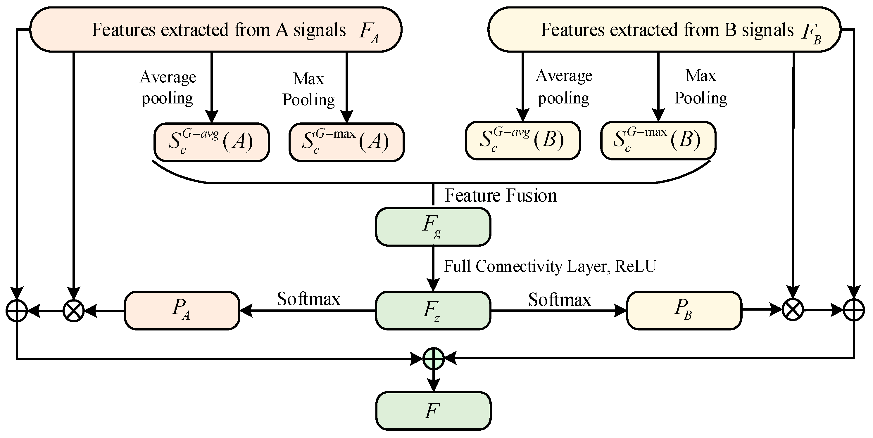
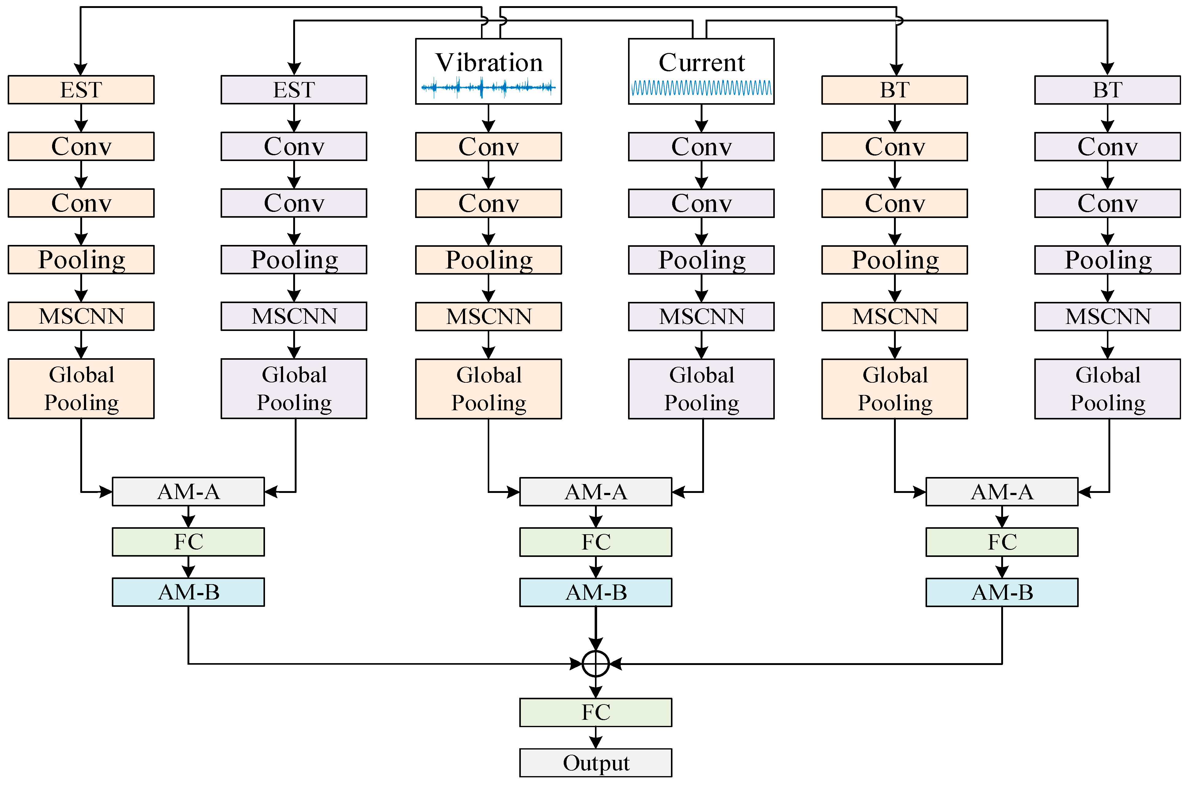
• An innovative multi-source feature fusion network is designed. This network leverages a multi-scale CNN, attention mechanism, and residual connections to extract fault features that are insensitive to changes in operating conditions. This approach enhances the model’s adaptability and facilitates the adaptive weighted fusion of information features, further improving fault-sensitive characteristics.

The overall architecture of this paper is shown in Figure 1. The subsequent Section 2 presents the M2IFD framework for fault diagnosis, followed by a detailed description of the two data transformation methods and the multi-source as well as multi-domain feature fusion network designed in this paper based on the attention mechanism. In Section 3, a comprehensive analysis of multiple comparative experiments was conducted using two different datasets. A conclusion and outlook of this study is presented in Section 4.

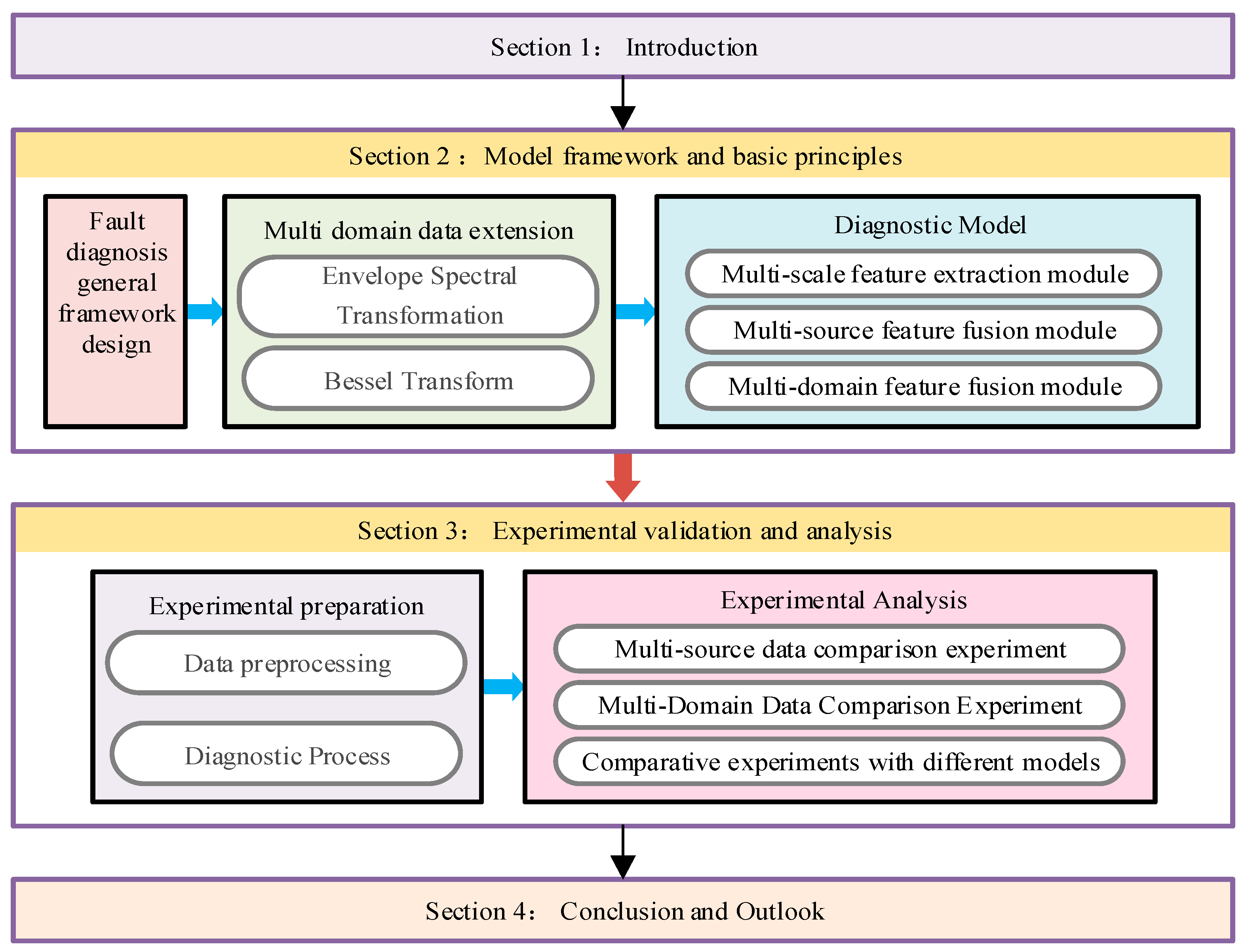
2. Model Framework and Basic Principles

2.1. Fault Diagnosis General Framework Design

The overall framework of the M2IFD in this paper is illustrated in Figure 2 and is primarily divided into three stages.

The first stage is the multi-domain conversion stage. To expand the effective information in the samples, the time domain signals collected and processed by sensors are converted into the frequency domain and time–frequency domain for subsequent analysis, and this paper selects the envelope spectral transform (EST) and the Bessel transform (BT) to analyze the frequency domain and the time–frequency domain, respectively. In frequency domain analysis, rolling bearing faults—particularly inner and outer ring defects or rolling body faults—often result in modulation effects in the vibration signal. The selection of the envelope spectral transform for frequency domain analysis effectively detects these modulation signals, resulting in high sensitivity to early failures [37]. In time–frequency domain analysis, the Bessel transform provides a joint time–frequency representation of the signal, enabling the capture of instantaneous frequency changes. Since rolling bearing fault signals are often non-smooth, the time–frequency analysis capability of the Bessel transform allows for effective processing and analysis of these signals. In addition, in the early stages of a fault, fault characteristics may be overwhelmed by background noise [38]. The high sensitivity of the envelope spectrum and the time–frequency fine analysis capability of the Bessel transform can effectively detect early faults. The combined utilization of time-domain analysis and the aforementioned transformation methods plays a complementary role in rolling bearing fault diagnosis, effectively enhancing the accuracy and reliability of fault identification.

The second stage involves performing multi-source feature extraction and fusion across each of the three domains. Given that each sensor type’s signal possesses unique physical meanings and characteristics in bearing fault diagnosis, directly mixing different types of data may lead to the loss of these unique attributes, thereby affecting the interpretability and effectiveness of the final model. The strategy adopted in this paper is to utilize the same model structure for feature extraction from each source individually, allowing for shared network parameter settings and hyperparameter tuning strategies. This approach reduces the number of parameters that require manual adjustment and mitigates the complexity of model design and training [39]. To extract sufficient and high-quality feature signals, a multi-scale convolutional neural network has been designed to ensure that each signal is adequately analyzed, capturing varying levels of information from subtle local features to global characteristics. Such consistency helps the model learn and extract valuable features from different signals more efficiently and improves the generalization ability of the model. Finally, a multi-source feature fusion network is designed based on the attention mechanism, so that the model adaptively realizes the adaptive weighted fusion of multi-source information features according to the differences in the sensitivity of different signal sources to different faults.

The third stage involves multi-domain feature fusion and fault classification output. Due to the inconsistency of information obtained from the fusion of multi-source data, the time-domain, frequency-domain, and time–frequency domain features derived from the feature extraction module typically cannot be directly fused. Therefore, this paper designs a multi-domain feature fusion module based on the attention mechanism, ultimately enabling accurate fault type determination and health status assessment based on the fused features for effective bearing fault diagnosis.

In the following section, we will describe the envelope spectral transform and Bessel transform in the first stage, the feature extraction module and the multi-source feature fusion module in the second stage, and the multi-domain feature fusion module in the third stage, respectively.

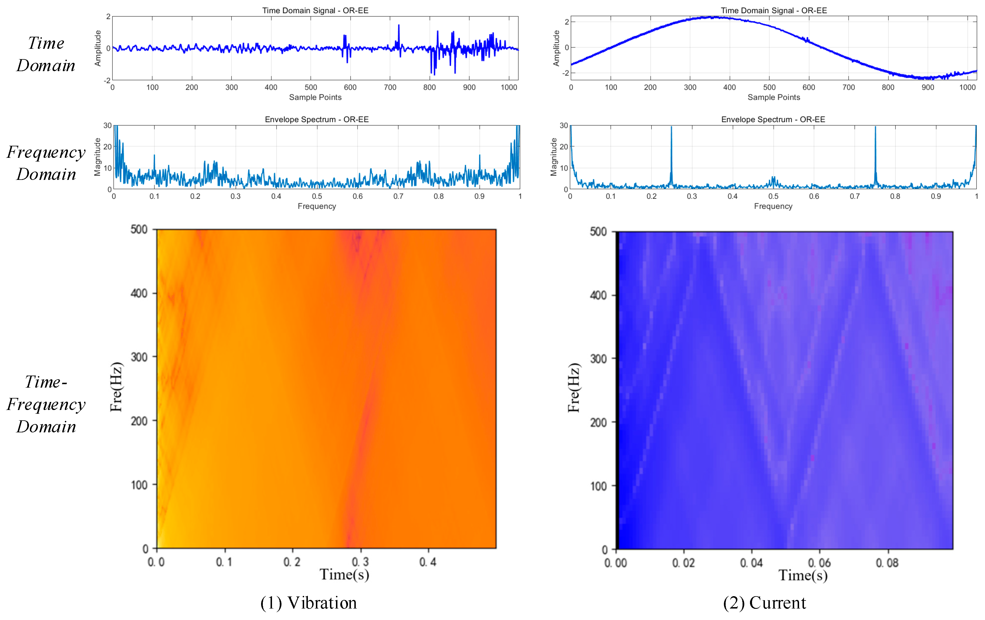
2.2. Multi-Domain Extension of Fault Data

The intrinsic vibration signals of motor bearings, as well as the motor current signals, are limited to the time domain. A single time-domain feature may not be able to adequately represent the fault characteristics. By representing data in different transform domains, different fault data attributes in different domains can be focused on from different perspectives, thus providing more valuable information. Fault characteristics under variable operating conditions may become less obvious or change due to changes in the environment or operating conditions. Multi-domain data representation allows for a more comprehensive capture of various fault characteristics that may arise under different operating conditions, resulting in improved adaptability and robustness of the model in practical applications. To gain a deeper understanding of the underlying structures of the original signals, we employ a variety of signal processing techniques that function across multiple domains. In this paper, the frequency domain conversion adopts the envelope spectral transform, and the time–frequency domain conversion adopts the Bessel transform, and the two transforms will be analyzed separately in the following.

(1)

Enveloped Spectral Transform

Envelope spectral transform is an important signal processing technique mainly used to analyze periodic or quasi-periodic signals. In practical fault diagnosis, the selection of the optimal frequency band and pre-filtering are crucial for enhancing the sensitivity of the envelope spectrum. This study employs the Fast Spectral Kurtosis (FSK) method to identify the resonance frequency band that contains the most significant fault-induced impulses. Following this, a Butterworth bandpass filter is applied to the raw signal within the identified frequency band to effectively suppress noise and irrelevant components. The envelope spectrum illustrates how the signal envelope appears in the frequency domain. It captures the changes in amplitude of the signal and serves as a depiction of its strength over time. Through the envelope spectrum, the modulation characteristics or amplitude modulation information of the signal can be better understood and analyzed [40]. The core of the envelope spectrum transform is the Hilbert transform as well as the Fourier transform, and its main steps are as follows:

In the first step, the original signal $x(t)$ is transformed to obtain the signal $h(t)$ by Hilbert transform, which is performed as follows:

$$h(t)=x(t)\ast {\displaystyle \frac{1}{\pi t}}={\displaystyle \frac{1}{\pi }}{\displaystyle {\int }_{-\infty }^{+\infty }\frac{x(\tau )}{t-\tau }}d\tau$$

(1)

where ∗ stands for convolution operation.

In the second step, the amplitude of the complex signal is calculated to obtain the envelope signal $x_{ht}(t)$:

$$x_{ht}(t)=\left|x(t)+jh(t)\right|$$

(2)

where $x(t)+jh(t)$ is the Hilbert transformed complex signal, the original signal $x(t)$ is the real part, and $h(t)$ after the Hilbert transform is the imaginary part.

In the third step, the envelope signal is Fourier transformed to obtain the envelope spectrum $E(t)$:

$$E(t)=\left|FT(x_{ht}(t))\right|$$

(3)

where FT stands for Fourier transform.

(2)

Bessel transform

To effectively address complex and non-stationary bearing fault signals, this paper introduces a novel time–frequency domain method known as the Bessel transform into the field of bearing fault diagnosis for converting both time-domain vibration and current signals into the time–frequency domain. The Bessel transform is realized by introducing a kernel constructed based on the Bessel function into Cohen’s class of distributions [41]. The Bessel kernel not only relies on high resolution to accurately capture instantaneous frequency variations when dealing with non-stationary signals but also reduces the effect of noise through its good smoothness characteristics. The general form of Cohen’s class of distributions is expressed as follows:

$$C(t,\omega ,\mathsf{\Phi })={\displaystyle \frac{1}{2\pi }}{\displaystyle \iiint e^{i(\xi \mu -\tau \omega -\xi t)}\mathsf{\Phi }(\xi ,\tau )f(\mu +\frac{\tau }{2})}f*(\mu -{\displaystyle \frac{\tau }{2}})d\mu d\tau d\xi$$

(4)

where $f(\mu )$ and $f*(\mu )$ are the original time signal and its complex conjugate, respectively, $\omega$ denotes the instantaneous frequency, $t$ denotes the instantaneous time, $\tau$ denotes the running time, $\xi$ denotes the frequency variable, which is used to obtain information in the frequency domain, $\mu$ is the positional variable related to the time delay, and $\mathsf{\Phi }(\xi ,\tau )$ is the kernel function, which determines the nature and characteristics of the time–frequency representation

$$\mathsf{\Phi }(\xi ,\tau )={\displaystyle \frac{J_1(2\pi \alpha \xi \tau )}{\pi \alpha \xi \tau }}$$

(5)

Among them, $J_1$ is the first type of Bessel function, and $\alpha$ is a scale factor greater than 0.

By integrating the Bessel kernel, the Bessel transform has a very good frequency resolution and can effectively capture the rapidly changing frequency components as well as subtle structural features in the signal. This means that it is capable of handling highly dynamic or non-stationary signals, providing rich time–frequency information.

2.3. Multi-Scale Feature Extraction Module

Considering the complex and varied characteristics of bearing signals—including non-smoothness, nonlinearity, and susceptibility to noise interference—neither smaller nor larger convolutional kernels can effectively capture features across all frequency ranges. Consequently, this paper presents a multi-scale convolutional neural network structure (MSCNN) as the foundational framework for modeling. Figure 3 illustrates the multi-scale convolutional neural network (MSCNN) structure proposed in this study. The design is inspired by the concept of multi-scale modeling in the field of computer vision: it integrates parallel convolution kernels from the GoogleNet Inception module for multi-scale feature fusion [42] and employs the 1 × 1 convolution method from ResNet for channel dimension compression [43]. These methods provide the theoretical foundation for the structural design of branches 1–3 in this study. Specifically, the design of the four branches is as follows: first, 1 × 1, 3 × 3, and 5 × 5 convolution kernels are used in branches 1–3, drawing on the inception module’s cross-scale feature capturing concept, while optimizing the kernel sizes for one-dimensional vibration signal processing to achieve multi-scale receptive field fusion. Second, 1 × 1 dimensionality reduction is employed in each branch to improve computational efficiency, inherited from ResNet’s bottleneck design. This reduces the number of parameters while preserving the ability to extract spatial features through convolutions. Additionally, an average pooling layer is included in branch 3 to retain local feature information in a balanced manner. Finally, in branch 4, deep feature enhancement is achieved through the continuous 3 × 3 convolution replacement strategy proposed by VGGNet [44]. Two 3 × 3 convolutions (equivalent to a 5 × 5 receptive field) replace larger kernels, increasing nonlinearity while reducing the number of parameters.

2.4. Feature Fusion Network Based on Attention Mechanism

When handling data from various sources, one may encounter issues of redundancy and correlation. These issues can introduce unnecessary noise during feature merging, adversely affecting the model’s performance. To address this issue, this paper introduces the attention mechanism to enhance the model’s effectiveness and robustness. The fundamental concept of the attention mechanism is to enhance the model’s performance by assigning weights to the importance of features. Specifically, the attention mechanism enables the model to automatically identify and emphasize features most relevant to the task, thereby minimizing the influence of redundant information. By concentrating on key features, it allows the model to extract crucial information from complex data more efficiently; consequently, the fusion performance can be significantly enhanced through the attention mechanism [45,46,47,48,49]. Furthermore, to prevent degradation issues arising from an increase in the number of model layers and to enhance the continuity of data flow, this paper introduces residual learning based on the attention mechanism to mitigate the problem of gradient vanishing and to improve training speed and accuracy. The multi-source feature fusion module designed in this paper is shown in Figure 4.

Assuming that $F_A$ and $F_B$ are features extracted from two different data sources, the fusion process is described in detail below in four steps:

Step 1: two different features are generated using global average pooling and global max pooling operations, respectively. The relevant formulas are as follows, and these two features can effectively complement each other for the subsequent attention mechanisms.

$$\left\{\begin{array}{c}{S}_c^{G-avg}(A)={\displaystyle \frac{1}{L}}{\displaystyle \sum _{i=1}^L{F}_A^c(i)}\\ S_c^{G-avg}(B)={\displaystyle \frac{1}{L}}{\displaystyle \sum _{i=1}^L{F}_B^c(i)}\end{array}\begin{array}{cc}& c=1,2,\dots ,M\end{array}\right.$$

(6)

$$\left\{\begin{array}{c}{S}_c^{G-\max }(A)={\max }_{i=1}^L{F}_A^c(i)\\ S_c^{G-\max }(B)={\max }_{i=1}^L{F}_B^c(i)\end{array}\begin{array}{cc}& c=1,2,\dots ,M\end{array}\right.$$

(7)

where $S_c^{G-avg}(A)$ and $S_c^{G-avg}(B)$ denote the global average pooling results of the cth channel of the compressed features of data A and data B, respectively. $S_c^{G-\max }(A)$ and $S_c^{G-\max }(B)$ denote the global max pooling results of the cth channel of compressed features for data A and data B; L is the total number of elements in the channel (i.e., feature map size, e.g., the width × height of the feature map); M denotes the number of feature channels; and $F_i^c$ denotes the value of the i-th element of the cth channel.

Step 2: combine the output features from Step 1 to generate a more expressive global feature representation. The combined global features are then input into a fully connected layer that further integrates these features to produce the final feature vector through linear transformation followed by the nonlinear activation function ReLU.

$$\left\{\begin{array}{c}{F}_g=[S_c^{G-avg}(A),S_c^{G-avg}(B),S_c^{G-\max }(A),S_c^{G-\max }(B)]\\ F_z=\sigma (W·F_g+b)\end{array}\right.$$

(8)

where $F_g$ is the compressed feature vector after global feature fusion; $F_z$ is the final fused global feature vector; W and b denote the weight matrix and bias term of the fully connected layer, respectively; $\sigma$ is the ReLU function.

Step 3: the soft attention mechanism enables the model to dynamically adjust the importance of input features based on the input by assigning varying weights to different segments of the input features, thereby allowing the model to concentrate on the most relevant information. That is, adaptive selection of channel features is achieved by applying the SoftMax function to the compact feature $F_z$ to generate the excitation signals $P_A$ and $P_B$. The SoftMax function is used to convert the input features into probability distributions to ensure that all the outputs add up to 1, and that the probability of excitation for each channel feature can be obtained adaptively:

$$\left\{\begin{array}{c}{P}_A={\displaystyle \frac{e^{W_A·F_Z}}{e^{W_A·F_Z}+e^{W_B·F_Z}}}\\ P_b={\displaystyle \frac{e^{W_B·F_Z}}{e^{W_A·F_Z}+e^{W_B·F_Z}}}\end{array}\right.$$

(9)

where $P_A$ and $P_B$ denote the excitation signals of $F_A$ and $F_B$, respectively. During feature fusion, excitation signals are applied to the feature vectors as weights, allowing more important features to contribute more significantly to the final output, while the influence of less important features is diminished. This mechanism enhances the model’s learning capability, thereby improving its performance.

Step 4: based on the excitation signals, i.e., the attention weights, obtained in Step 3, the importance of different signals is dynamically adjusted to ensure that more significant signals hold greater weight in the fused features, while the influence of less important signals is diminished. Meanwhile, to prevent the loss of original features, a residual connection is introduced, wherein the original data are directly linked to the data refined by the attention mechanism. Residual connections facilitate smoother gradient propagation, particularly in deep networks, thereby alleviating the issues of vanishing or exploding gradients. As a result of smoother gradient flow, the network typically trains faster, reducing training time and effectively mitigating potential degradation of the model:

$$F=(P_A\otimes F_A+F_A)+(P_B\otimes F_B+F_B)$$

(10)

where F is the fusion feature, and $\otimes$ denotes element-by-element multiplication in the channel domain.

2.5. Multi-Domain Feature Fusion Module Based on Attention Mechanism

Given that the features obtained from different domains often exhibit significant differences and cannot be directly concatenated or fused, an attention mechanism combined with residual connections is introduced in this section of the multi-domain feature fusion module, as illustrated in Figure 5. The input time domain, frequency domain, and time–frequency domain features are set to be $F_1$, $F_2$, $F_3$, respectively, and each feature is first pooled globally on average to generate a compact feature representation $Avg(F_i)$, where $F_i$ is the feature extracted from the first $i$ domain. Subsequently, the pooled features are transformed by two fully connected layers, The fully connected layer W1 combines the ReLU activation function to introduce nonlinearity to enhance complex feature learning, and the fully connected layer W2 combines the Sigmoid activation function to generate attention weights, and the Sigmoid mainly maps the features to the [0, 1] interval to adjust the importance of the features, and finally the generated attention weights are multiplied with the original features element by element to enhance the important features, and subsequently, the result is summed with the original features to obtain the output feature $G_i$ to realize the jump connection to retain the original information; the total formula is as follows:

$$G_i=(\sigma W_2\delta (W_{1}Avg(F_i)))\otimes F_i+F_i$$

(11)

where Avg denotes the global pooling operation, $W_1$ and $W_2$ denote the two fully connected layer weight coefficients, respectively, $\delta$ denotes the ReLU activation function, $\sigma$ denotes the Sigmoid activation function, and $\otimes$ denotes the element-by-element multiplication. After the above process, the module dynamically evaluates and weights the importance of the features through the attention mechanism so as to map the features from different domains into a unified representation space, obtains the attention-weighted feature $G_i$ from each domain so that these features can be compared and fused on the same basis, and subsequently compresses these feature vectors into fixed-length feature representations through a global average pooling operation so that they can be directly spliced in the channel dimension. Eventually, these feature channels are concatenated to enable multi-domain feature fusion. By merging various features, the model can develop more complex representations of features, resulting in improved final performance.

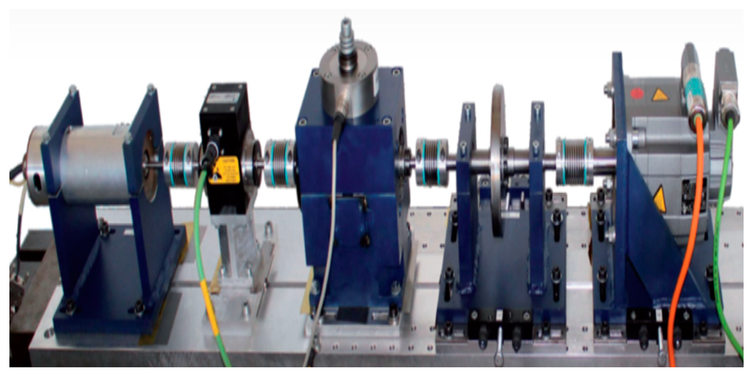
3. Experimental Verification and Results Analysis

In this section, the effectiveness of the proposed model is evaluated using two bearing datasets. The first dataset is derived from the publicly available repository of Paderborn University, while the second dataset originates from the bearing dataset curated by the Department of Mechanical Engineering at the Korea Advanced Institute of Science and Technology (KAIST).

3.1. CASE 1

3.1.1. Data Preprocessing for CASE1

The experimental dataset utilized in this study is the bearing dataset from the University of Paderborn, Germany [50]. The relevant experimental setup is shown in Figure 6. The experimental platform employs deep groove ball bearings of type 6203 as test subjects. The phase currents of the motor are measured using LEM CKSR 15-np type current sensors (LEM, Groß-Gerau. Germany), and the analog signals are converted to digital signals at a sampling rate of 64 kHz. The vibration signals were measured using a piezoelectric accelerometer (type 336C04; PCB Piezotronics, Inc., Depew, NY, USA) and a charge amplifier (type 5015A; Kistler Group, Sindelfingen, Germany), both synchronized at a sampling rate of 64 kHz. Both the motor current signals and the vibration signals were consistently measured synchronously to accurately record the operating conditions. The operational temperature of the bearing and test rig, primarily caused by friction during vibration testing, was maintained within 45 °C to 50 °C throughout the experiments.

In this paper, we select healthy bearings, three types of outer-ring failures, and two types of inner-ring failures for experimental verification, resulting in a total of six bearing states, denoted as 0 to 5, as shown in

Table 1. Classification label for CASE1.

Types of Failures	Tags
Healthy	0
OR-EDM	1
OR-EE	2
OR-Drilling	3
IR-EDM	4
IR-EE	5

. Specifically, EDM represents artificial damage simulation through electric discharge, while EE represents artificial damage simulation through electric engraving. OR and IR refer to the outer and inner rings of the bearings, respectively. The specific manifestations of the three fault types are illustrated in Figure 7.

To investigate the diagnostic capability of the model under varying operating conditions, we selected three operating conditions—A, B, and C (as shown in

Table 2. Different conditions of bearings.

	Speed (rpm)	Load Torque (N/m)	Radial Force (N)
A	900	0.7	1000
B	1500	0.7	1000
C	1500	0.7	400

)—for subsequent experiments.

Due to the large volume of acquired data, preprocessing is required to optimize the model inputs. First, the signals are sliced and overlapped. Each sample contains 1024 data points, with the next sample segment starting from the 769th data point of the current segment (i.e., the first 256 data points are overlapped), followed by collecting another 1024 data points as a new sample. This overlapping sampling method produces smoother transitions and captures more signal features, thereby avoiding the loss of key information during slicing.

To achieve the multi-source fusion previously mentioned, the original time-domain signal samples undergo envelope spectral transformation and Bessel transformation, respectively. The preprocessing pipeline operates as follows: vibration/current signals are bandpass-filtered (Butterworth 5th-order, 1–20 kHz) prior to envelope spectral transformation (EST), which generates frequency-domain features through the Hilbert transform and 1024-point FFT (512 frequency bins). Bessel transformation employs a 6th-order low-pass filter (12 kHz cutoff) to preserve transient impulses. Time-domain features (peak-to-peak, RMS, kurtosis, and crest factor) are extracted from raw 1024-sample segments, while Bessel-based time–frequency maps (128 × 128 pixels) capture the joint time–frequency energy distribution. Each M2IFD input integrates 4 (time) + 512 (frequency) + 16,384 (time–frequency) = 16,900 multi-domain features. The time-domain, frequency-domain, and time–frequency-domain sample intercepts generated from the vibration signal data of the outer ring electrodynamic sculpture and the single-ended current signal under the selected operating condition A are presented in Figure 8. The frequency-domain signal image, which was transformed by the envelope spectral transformation, is shown for the convenience of displaying the zoomed-in segment from the intercepts.

Furthermore, to evaluate the generalization performance of the model under various training and testing conditions, as well as its ability to adapt to unknown operating conditions, the aforementioned three operating conditions are paired two by two to generate cross-condition training and testing sets, aiming to evaluate whether the model can maintain good predictive performance under unknown operating conditions. The specific groupings are presented in

Table 3. Experimental grouping.

Experiment Name	Training Dataset	Testing Dataset	Number of Samples
AB	A	B	40,000
AC	A	C	40,000
BA	B	A	40,000
BC	B	C	40,000
CA	C	A	40,000
CB	C	B	40,000

.

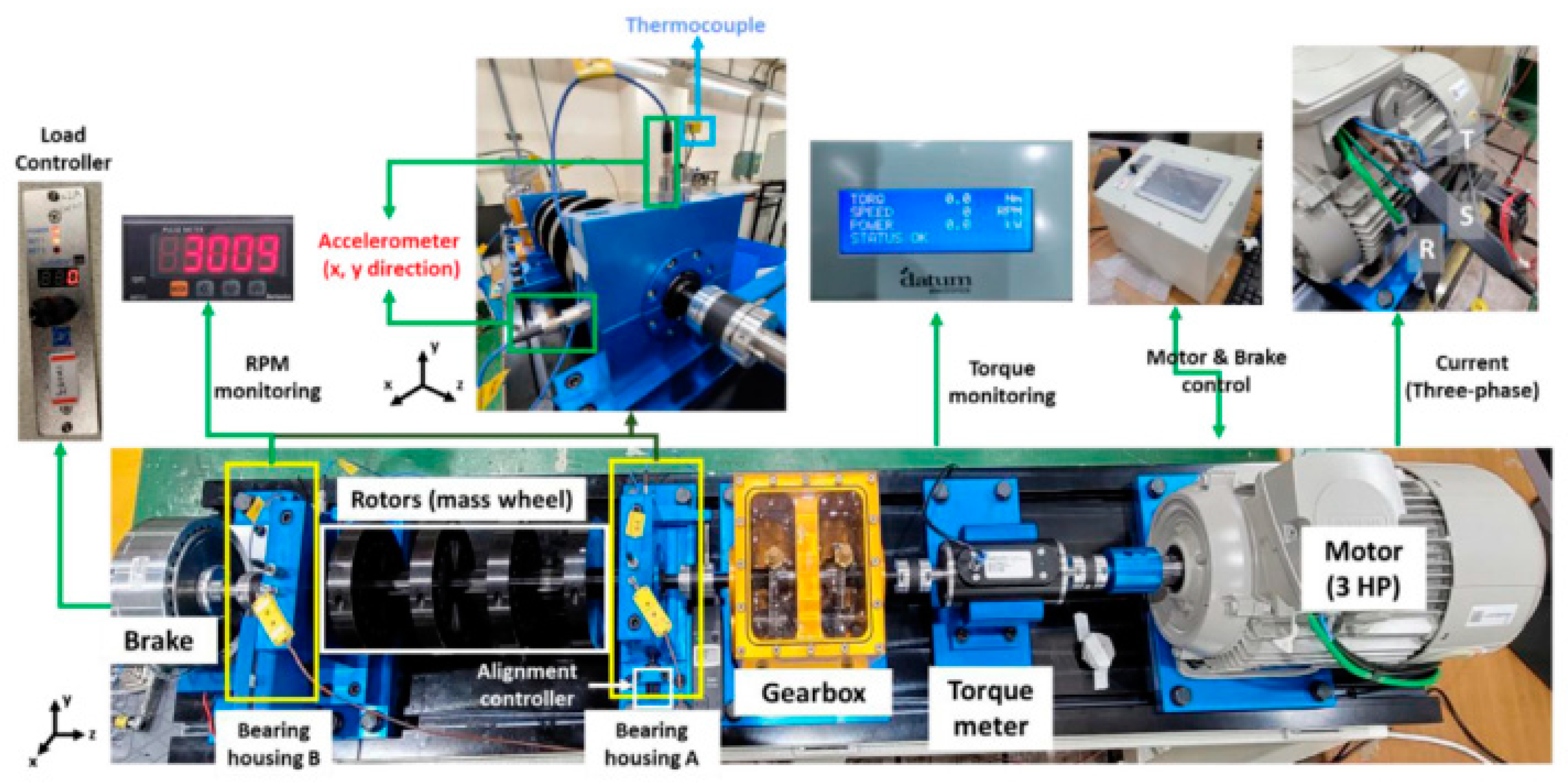
3.1.2. Overview of Specific Experimental Parameters

The experimental setup was executed using the Python 3.9 programming language within the PyTorch 1.12.0 framework. The computations were performed on a machine equipped with an NVIDIA 1660 GPU and 16 GB of RAM. The structure of the fault diagnosis model M2IFD proposed in this paper is illustrated in Figure 9.

The input signals consist of both vibration and current signals. For each signal, the model extracts and fuses features across three distinct domains: time, frequency, and time–frequency. Each domain subsequently compresses the spatial dimensions of the features through global pooling, resulting in a comprehensive global feature representation. In this step, the features of each domain of each signal are extracted and used as input for subsequent fusion. Subsequently, the multi-source data from each domain is fed into the multi-source feature fusion module AM-A. This process yields the fused feature outputs of the vibration and current signals across the three domains, which are then further compressed and tightly mapped by the fully connected layer. This is followed by the multi-domain feature fusion module AM-B, which employs an attention-based weighting mechanism to dynamically assign domain importance weights. Specifically, for features $F_i$ from the i-th domain, the weight ${\alpha }_i$ is calculated as follows:

$${\alpha }_i={\displaystyle \frac{e^{W_{\alpha }·F_i+b_{\alpha }}}{{\displaystyle {\sum }_{j=1}^D{e}^{W_{\alpha }·F_j+b_{\alpha }}}}}$$

(12)

$$F_{fused}={\displaystyle {\sum }_{i=1}^D{\alpha }_i{F}_i}$$

(13)

where $W_{\alpha }$ and $b_{\alpha }$ are learnable parameters, and D is the number of domains. The fused feature is then obtained by Formula (13). This adaptive weighting strategy allows the model to prioritize domain-specific features under varying operating conditions, thereby enhancing diagnostic robustness.

The final six-class fault diagnosis results are produced by the output layer. The specific detailed parameters of the M2IFD model are presented in

Table 4. The specific detailed parameters of the M2IFD.

Layer Name	Kernel Size/Step	Type
Conv1	3 × 1/2	BN-Relu
Conv1	2 × 1/2	BN-Relu
Pooling	2 × 1/2	MAXpool
Conv_a	1 × 1/2	BN-Relu
Conv_b	1 × 1/1	BN-Relu
Conv_b	3 × 1/2	BN-Relu
Average Pooling_c	3 × 1/2	BN-Relu
Conv_c	1 × 1/1	BN-Relu
Conv_c	5 × 1/1	BN-Relu
Conv_d	1 × 1/1	BN-Relu
Conv_d	3 × 1/1	BN-Relu
Conv_d	3 × 1/2	BN-Relu
Global Pooling	3 × 1/1	BN-Relu

.

During the model training process, the batch size is set to 128, and the learning rate is configured at 0.01. If the model does not improve the recognition accuracy on the test set for six consecutive epochs, training is halted to prevent overfitting. Conversely, if the recognition accuracy on the validation set in the current epoch exceeds the previous highest accuracy, the current recognition accuracy is recorded as the new highest accuracy, and the counter is reset to zero. This indicates that there is still potential for model improvement, and therefore, training is not terminated. Additionally, the parameters of the most recent model iteration are saved to preserve the optimal model. The loss function used is the negative log-likelihood loss function (NLLLoss). Prior to the use of NLLLoss, the output of the model is usually processed to generate a probability distribution by means of a softmax function, and subsequently NLLLoss reduces the discrepancy between the predicted results and the true labels by calculating the negative logarithmic value of the log-likelihood of the model’s output with respect to the true category. Its formula is as follows:

$$NLLL\mathit{oss}(y,\overline{y})=-{\displaystyle \sum _{t=1}^C{y}_i\log ({\overline{y}}_i)}$$

(14)

where C is the total number of categories, and y is the one-hot encoding of the true label, where $\overline{y}$ is the output of the model after softmax processing and represents the predicted probability of each category.

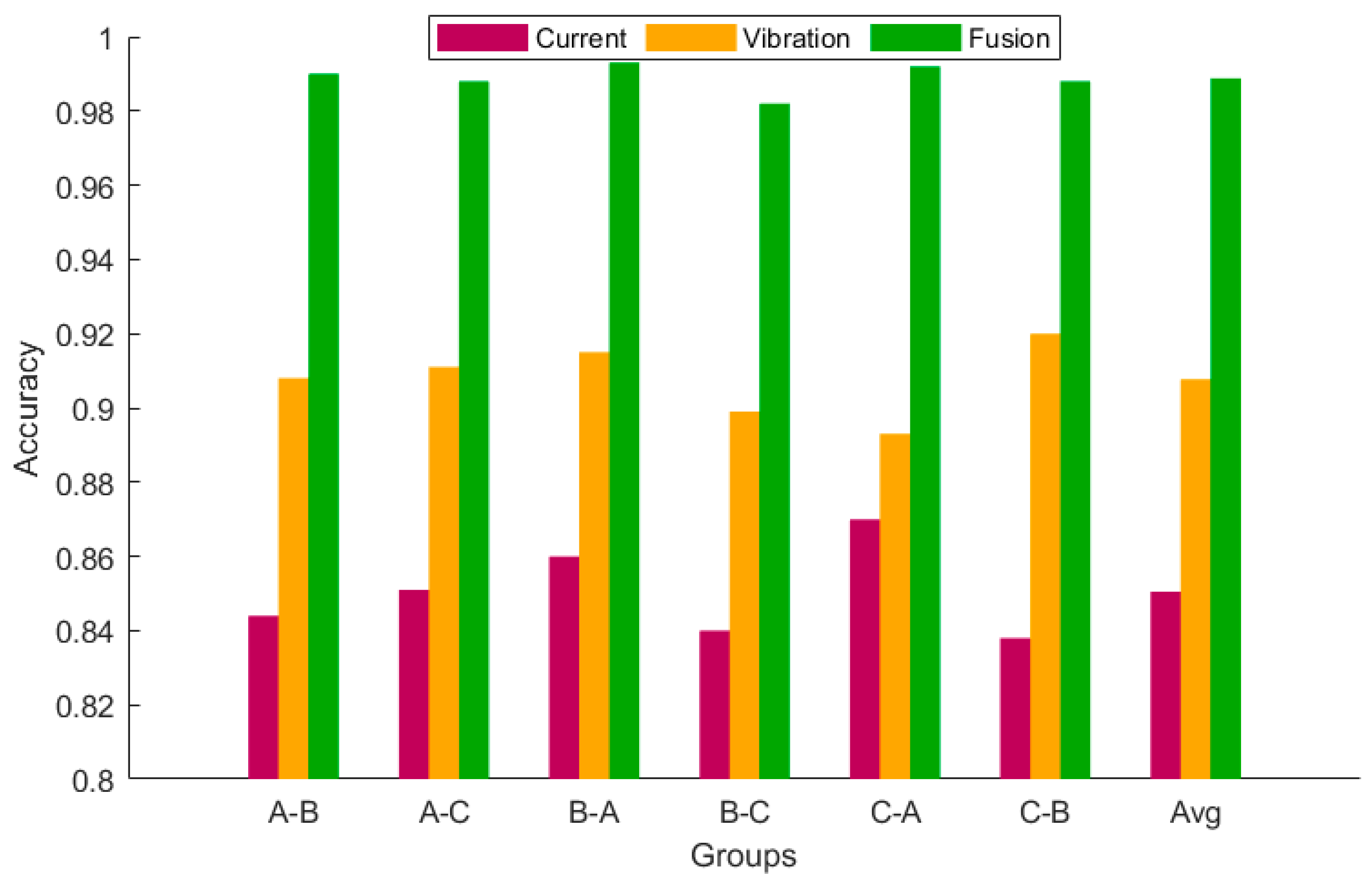
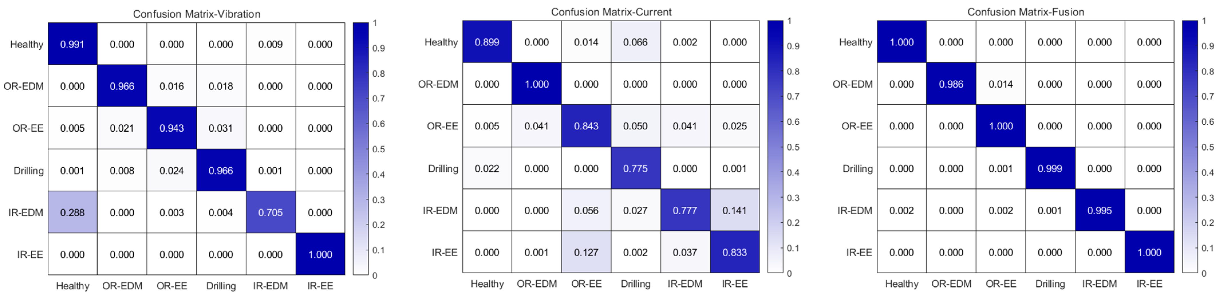
3.1.3. Multi-Source Data Comparison Experiment

The first comparative experiment conducted in this study is a multi-source data comparison experiment, implemented as follows: first, the raw time-domain data from the vibration and current signals are utilized separately and input into the feature extraction module for experimental analysis. Subsequently, the data from the vibration and current signals are fused and analyzed through the feature extraction module and the multi-source feature fusion module. The comparative histograms of the experimental results are presented in Figure 10. Additionally, the experimental results are visualized using a normalized confusion matrix, where each row represents the proportion of samples within a given category predicted to belong to each category. The results of this experimental confusion matrix are shown in Figure 11.

The experimental results indicate that using the current signal alone for fault diagnosis yields the lowest average accuracy of only 85.05%. In contrast, when utilizing only the vibration signal, the accuracy improves slightly to 90.77%. Furthermore, when both the vibration and current signals are employed for fault diagnosis via the multi-source feature fusion network, the accuracy significantly increases to 98.88%, surpassing that of either input alone. This demonstrates that the accuracy reaches as high as 98.88%. The confusion matrix further demonstrates that when using either current signals or vibration signals in isolation, samples from specific categories tend to be misclassified as belonging to other categories, highlighting the limited feature representation capability of a single signal. Following the application of multi-source information fusion, the values of the diagonal elements in the confusion matrix approach 1, which indicates that the model achieves a high classification accuracy for each category, while the classification error rate is significantly reduced. It is noteworthy that in the vibration signal confusion matrix, the IR-EDM category is misclassified as “Healthy” with a relatively high probability (28.8%), whereas this does not occur in the current and mixed signals. This suggests that the vibration characteristics produced by IR-EDM may have a higher similarity to the characteristics of the healthy state. This highlights the limitations of using a single vibration signal for specific fault diagnosis, while multi-sensor fusion compensates for this drawback by supplementing multi-dimensional information.

It can be concluded that multi-source information fusion provides significant advantages in bearing fault diagnosis. This indicates that a single signal is insufficient to capture all relevant fault information, while the combination of both signals not only offers a more comprehensive representation of the fault but also enables the model to learn a richer and more discriminative feature set.

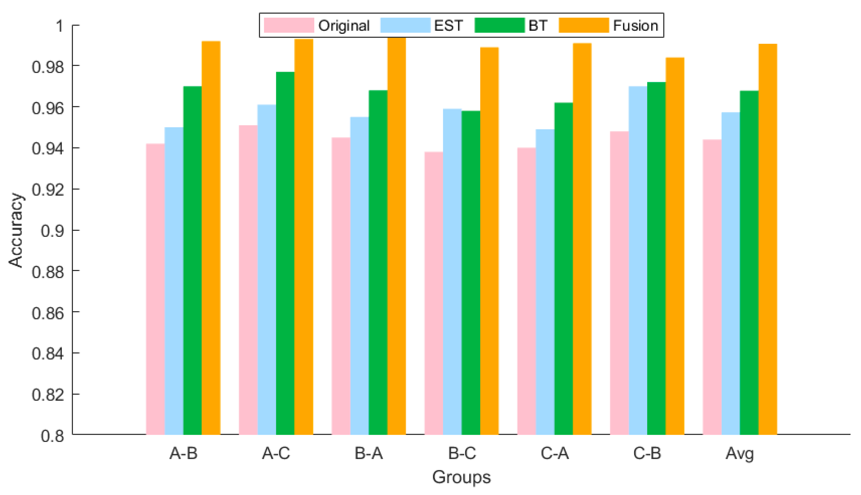
3.1.4. Comparative Experimental Analysis of Multi-Transform Domain Data for CASE1

The second comparative experiment in this study focuses on the multi-transform domain data comparison, with the specific implementation steps outlined as follows: four comparative experiments are established within each experimental group. First, the original time-domain data, frequency-domain data obtained through envelope spectral transformation, and time–frequency-domain data derived from Bessel transformation are individually input into the feature extraction and multi-source feature fusion network for analysis. Finally, these three types of data are fused across domains using the multi-source feature fusion network and the multi-domain feature fusion module, followed by experimental analysis. The comparative histograms of the experimental results, along with their corresponding confusion matrices, are presented in Figure 12 and Figure 13.

The experiment shows that when the time domain, frequency domain, and time–frequency domain data are used as inputs alone, the average accuracy of the three is 94.40%, 95.73%, and 96.78%, respectively, which is high, and the time–frequency domain data obtained by Bessel transform has a certain weak advantage compared with the other two groups from the three transform domains. After the data features of the three transform domains are fused by the multi-domain data fusion, the accuracy rate reaches 99.11%, which is much higher than that of the three-domain data as input alone.

Therefore, it can be concluded that the multi-domain data fusion strategy has a significant advantage in fault diagnosis, which realizes higher diagnostic accuracy by integrating the features of the time domain, the frequency domain, and the time–frequency domain, and makes up for the shortcomings of the features of a single domain through fusion, realizing the complementary nature of the information, so that the model can better adapt to the complex and changing failure modes.

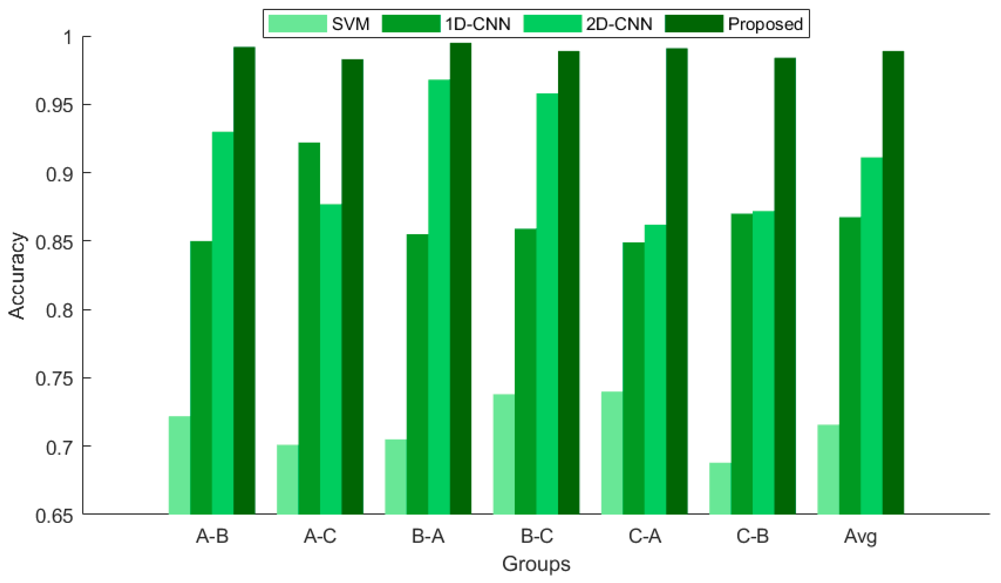
3.1.5. Comparative Experimental Analysis of Different Models for CASE1

This paper presents two experiments in Section 3.1.3 and Section 3.1.4 that validate the significant advantages of the multi-source fusion and multi-domain fusion fault diagnosis models based on the attention mechanism in enhancing fault identification capability. To further assess the superiority of the M2IFD model, comparative experiments with classical fault diagnosis methods are also conducted in this study, aiming to explore fault diagnosis performance across different inputs and model design strategies.

To ensure fair and effective comparative experiments, the following classical methods are selected and evaluated under uniform experimental conditions in this study: (1) SVM: by employing Empirical Mode Decomposition (EMD), the vibration and current signals are decomposed into Intrinsic Mode Functions (IMFs). The kurtosis values of the first five IMF components are extracted as feature vectors and input into a Support Vector Machine (SVM). A kernel function is utilized to map the data into a high-dimensional space for model training, ultimately achieving fault classification. (2) 1D-CNN: integration of features from multi-source data at specific fusion points. (3) 2D-CNN: time–frequency domain features are extracted from images using a 2D convolutional network after converting time-series data into 2D grayscale images, followed by data fusion performed in the image space. To ensure fairness in the model comparison experiments, a uniform dataset, consistent sample division, and identical hyper-parameter settings are employed, with the results presented in the histogram shown in Figure 14.

In the experiments conducted, comparison of the classification accuracies of various fault diagnosis methods reveals that the average accuracy of the traditional Support Vector Machine (SVM) method is merely 71.57%. This result clearly demonstrates that traditional classification methods are insufficient to address the increasingly complex needs of fault diagnosis and struggle to provide reliable fault identification. Consequently, there is an urgent need to adopt more advanced and effective techniques to enhance the accuracy and robustness of fault diagnosis.

With the introduction of deep learning methods for feature extraction utilizing 1D-CNN and 2D-CNN, the average feature recognition accuracies of these two methods are observed to be 86.75% and 91.12%, respectively. This indicates that deep learning techniques are more effective in automatically extracting and learning complex features compared to traditional methods. Particularly when dealing with signal data of a temporal nature, deep learning models can capture nonlinear relationships and local features within the data. This significant improvement further underscores the capabilities of deep learning methods in feature representation and pattern recognition.

However, when compared to the aforementioned deep learning models, the M2IFD method proposed in this study exhibits superior performance, achieving an average accuracy of 98.90%. This notable improvement not only demonstrates the effectiveness of multi-source information fusion but also indicates that integrating features from various signal sources allows for the acquisition of more comprehensive and enriched fault information. This result illustrates that traditional single-signal feature extraction methods struggle to meet the diagnostic requirements of complex faults under variable operating conditions, while the multi-source feature fusion model effectively enhances diagnostic accuracy.

3.2. CASE 2

3.2.1. Data Preprocessing for CASE2

In Case 2, the bearing dataset provided by the Department of Mechanical Engineering at the Korea Advanced Institute of Science and Technology is utilized [51]. The test rig for the dataset is shown in Figure 15. The vibration signals of NSK 6205 DDU bearings are acquired using a PCB352C34 accelerometer model (PCB Piezotronics, Inc., Depew, NY, USA), while the current signals are captured via an NI9775 module (National Instruments, Austin, TX, USA). These data are collected under three distinct load conditions (0 Nm, 2 Nm, and 4 Nm), respectively named X, Y, and Z. Various experimental groups are delineated as shown in

Table 5. Experimental grouping for Case 2.

Experiment Name	Training Dataset	Testing Dataset	Number of Samples
XY	X	Y	2000
XZ	X	Z	2000
YX	Y	X	2000
YZ	Y	Z	2000
ZX	Z	X	2000
ZY	Z	Y	2000

. In the variable load condition tests, bearing faults are simulated according to crack sizes of 0.3 mm, 1.0 mm, and 3.0 mm, encompassing both inner ring faults and outer ring faults. The corresponding labels are comprehensively detailed in

Table 6. Classification label for CASE2.

Types of Failures	Tags
Healthy	0
OR-0.3	1
OR-1	2
OR-3	3
IR-0.3	4
IR-1	5
IR-3	6

.

In a manner analogous to Case 1, the adaptability of the model to various operating conditions was assessed. Similarly, the vibration and current signals were overlaid and segmented, with 1024 data samples being collected for every 768 data points. For each bearing operating condition, a total of 2000 sample data points were gathered for both training and testing purposes.

The architecture and parameters of the deep network employed in Case 2 are identical to those utilized in Case 1. Consequently, the results of the performance analysis and comparison are presented directly.

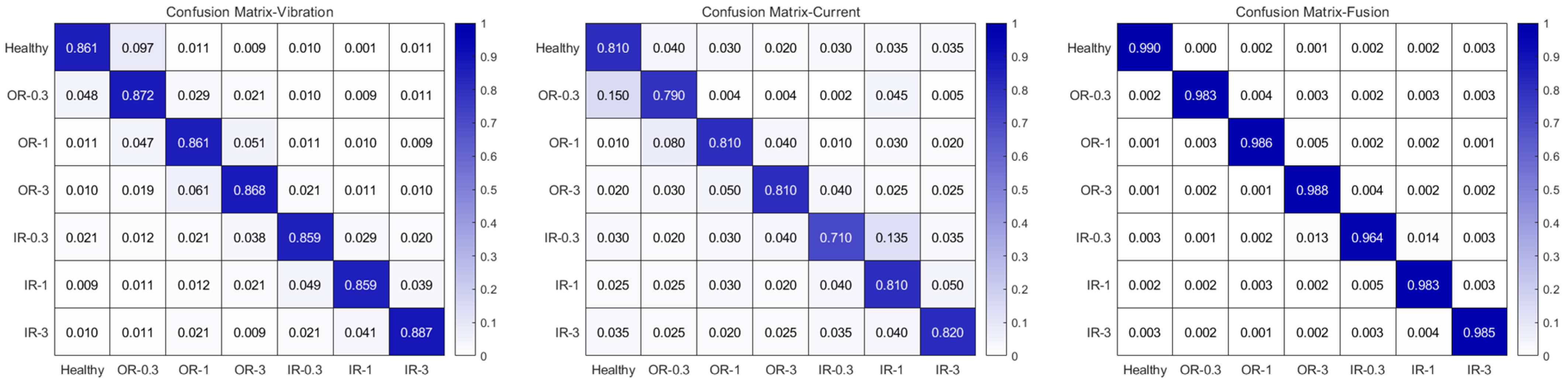
3.2.2. Comparative Experimental Analysis of Multi-Source Data

Analogous to Case 1, the initial comparative experiment involves a multi-source data comparison, in which data from individual sensor types are input separately as well as in combination. Figure 16 and Figure 17 illustrate the comparative histograms and confusion matrices of the experimental results, respectively. The findings reveal that the accuracy is 82.62% for current signals and 90.81% for vibration signals when input individually, which is markedly lower than the 98.38% achieved with combined inputs. This underscores the significance of integrating data from multiple sources to enhance the performance and reliability of diagnostic models. Therefore, for applications that demand high accuracy, prioritizing the use of combined sensor data over reliance on data from a single source is advisable.

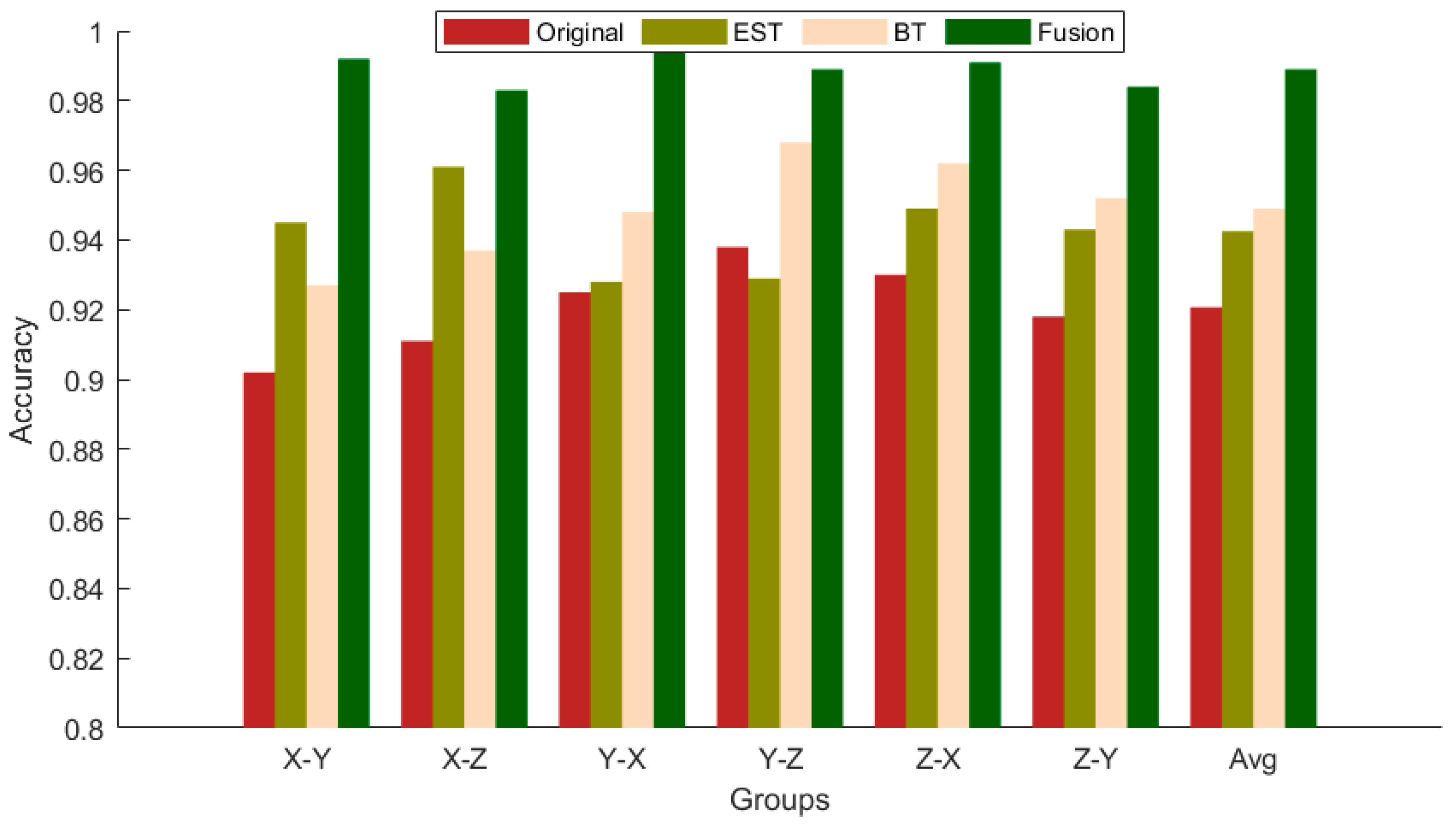
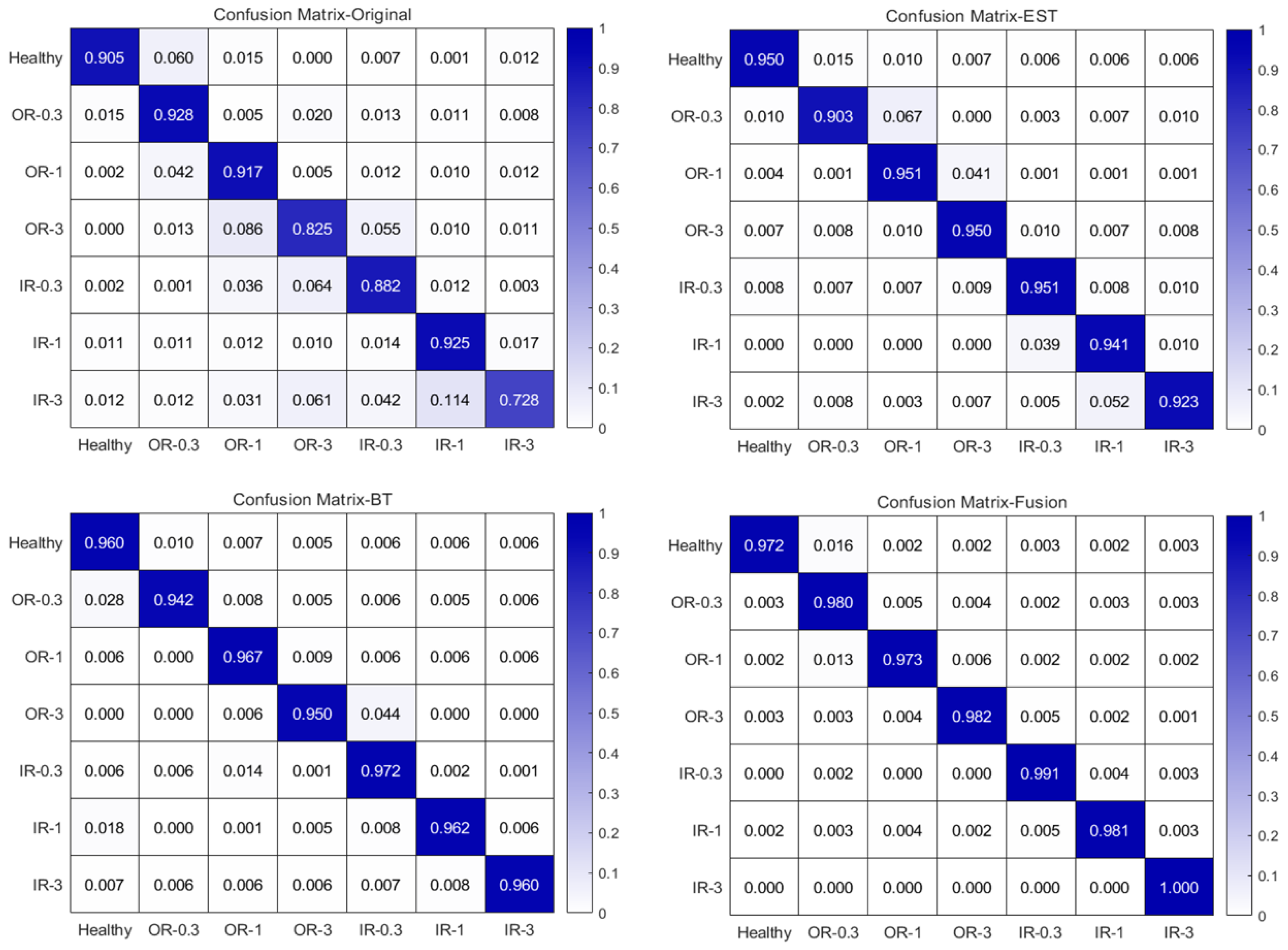
3.2.3. Comparative Experimental Analysis of Multi-Transform Domain Data for CASE2

The second comparative experiment involves a multi-domain data comparison. This experiment evaluates the impact of multiple transformation domains on the model by comparing the outcomes of using single-domain features against those achieved by fusing multi-domain features. Figure 18 illustrates the comparative histograms of the experimental results, while Figure 19 presents the confusion matrix. The findings reveal that the accuracy is 92.07% without domain transformation. With envelope spectrum transformation and Bessel transformation, the accuracy rises to 94.25% and 94.9%, respectively. Nevertheless, the highest accuracy of 98.9% is attained when multi-domain data are fused. This corroborates the conclusions drawn in CASE 1, demonstrating that acquiring information from multiple transformed domains offers a more comprehensive representation of the data, thereby enhancing the robustness and reliability of the diagnosis. Consequently, integrating multi-domain data should be regarded as a critical step in developing high-precision diagnostic models.

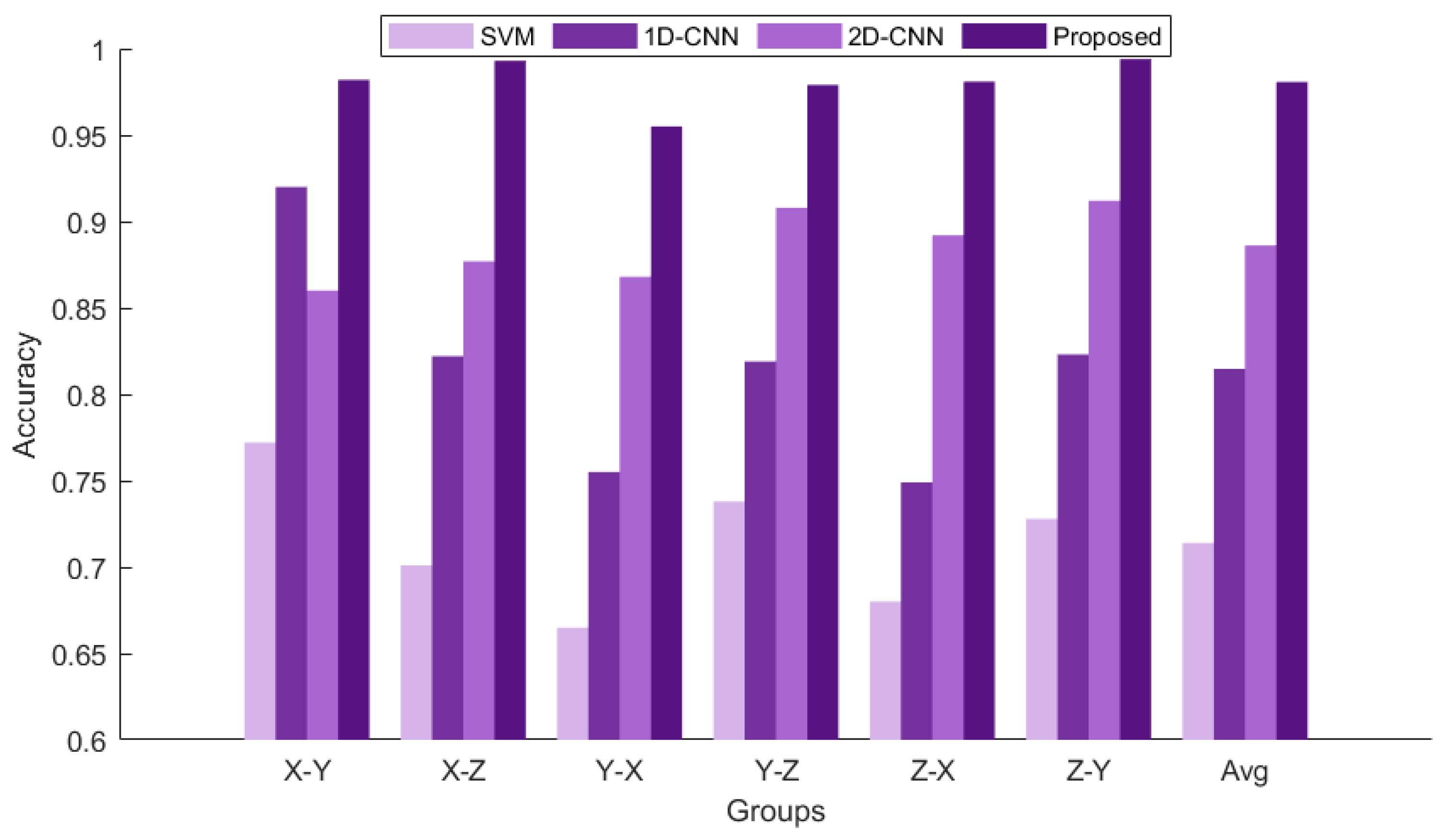
3.2.4. Comparative Experimental Analysis of Different Models

Similarly to Case 1, several other methods referenced in Case 1 are selected here for comparison. The experimental results are then depicted in a histogram, as shown in Figure 20, further validating the conclusions drawn earlier.

4. Conclusions

This paper proposes a bearing fault diagnosis method that integrates multi-source information fusion and multi-domain information fusion, referred to as M2IFD. This method facilitates efficient identification of bearing faults through the incorporation of the attention mechanism, envelope spectral transform, and Bessel transform. The method comprises three primary stages: First, the original signal is transformed into frequency and time–frequency domains using various signal transformation techniques to extract richer fault features. Second, features are independently extracted in each transform domain and fused through a multi-source feature fusion model based on the channel attention mechanism, preserving the unique information of each signal source. Lastly, a multi-domain feature fusion model is employed for cross-transform domain fusion.

Finally, extensive experimental comparisons and analyses were conducted based on the Paderborn dataset in Germany and the Korea Advanced Institute of Science and Technology bearing dataset, and the results indicate that the proposed method achieves high accuracy under various working conditions, demonstrating good adaptability and robustness. Notably, the integration of multi-source data and multi-transform domain analysis not only enhances the comprehensiveness and accuracy of fault diagnosis but also demonstrates strong adaptability under varying operating conditions.

Future research will primarily focus on the following aspects for further exploration: the first aspect involves the expansion and diversification of the dataset. To further verify the model’s applicability and generalization capability, experiments should be conducted on different types of equipment exhibiting a wider range of failure modes, particularly accounting for the impact of various environmental noise and changes in working conditions. The second aspect involves addressing model complexity and interpretability, as well as enhancing the model’s deployability in practical applications by reducing the number of parameters or designing a more lightweight network structure.

References

1. Xiao, Q.; Yang, M.; Yan, J.; Shi, W. Feature decoupling integrated domain generalization network for bearing fault diagnosis under unknown operating conditions. Sci. Rep. 2024, 14, 30848. [Google Scholar] [CrossRef]
2. Sun, Y.; Tao, H.; Stojanovic, V. Pseudo-label guided dual classifier domain adversarial network for unsupervised cross-domain fault diagnosis with small samples. Adv. Eng. Inform. 2025, 64, 102986. [Google Scholar] [CrossRef]
3. Qiao, Z.; Yao, D.; Yang, J.; Zhou, T.; Ge, T. MSTD: A framework for rolling bearing fault diagnosis based on multi-scale and soft-threshold denoising. Nondestruct. Test. Eval. 2024, 1–21. [Google Scholar] [CrossRef]
4. Zeng, L.; Chang, X.; Chen, J.; Wang, S. An Auxiliary Branch Semi-supervised Domain Generalization Network for Unseen Working Conditions Bearing Fault Diagnosis. IEEE Sens. J. 2024, 24, 42327–42342. [Google Scholar] [CrossRef]
5. Snyder, Q.; Jiang, Q. Integrating self-attention mechanisms in deep learning: A novel dual-head ensemble transformer with its application to bearing fault diagnosis. Signal Process. 2025, 227, 109683. [Google Scholar] [CrossRef]
6. Zheng, Y.; Li, W.; He, G.; Ding, K.; Chen, Z. Natural Modal Sketching Network: An Interpretable Approach for Bearing Impulsive Feature Extraction. IEEE Trans. Cybern. 2024, 55, 953–968. [Google Scholar] [CrossRef]
7. Jiang, L.; Shi, C.; Sheng, H.; Li, X.; Yang, T. Lightweight CNN architecture design for rolling bearing fault diagnosis. Meas. Sci. Technol. 2024, 35, 126142. [Google Scholar] [CrossRef]
8. Zhao, X.; Guo, H. Rolling bearing fault diagnosis model based on DSCB-NFAM. Meas. Sci. Technol. 2023, 35, 015029. [Google Scholar] [CrossRef]
9. Zhang, D.; Gong, Z.; Zhou, H.; Ma, S.; Li, T.; Huang, Y.; Hu, X. Enhanced Wavelet Transform-Integrated MWRC-ResNet: A Novel Framework for Interpretable and Noise-Robust Rolling Bearing Fault Diagnosis. Meas. Sci. Technol. 2025, 36, 026102. [Google Scholar] [CrossRef]
10. Song, L.; Lin, T.; Jin, Y.; Zhao, S.; Li, Y.; Wang, H. Advancements in Bearing Remaining Useful Life Prediction Methods: A Comprehensive Review. Meas. Sci. Technol. 2024, 35, 092003. [Google Scholar] [CrossRef]
11. Chen, Y.; Shi, J.; Shen, C.; Huang, W.; Zhu, Z. CycleGAN With Momentum Control for Intelligent Bearing Fault Diagnosis Driven by Dynamic Models. IEEE Sens. J. 2024, 24, 39315–39324. [Google Scholar] [CrossRef]
12. Li, X.; Wang, Y.; Zhao, S.; Yao, J.; Li, M. Adaptive Convergent Visibility Graph Network: An interpretable method for intelligent rolling bearing diagnosis. Mech. Syst. Signal Process. 2025, 222, 111761. [Google Scholar] [CrossRef]
13. Zhang, M.; He, C.; Huang, C.; Yang, J. A weighted time embedding transformer network for remaining useful life prediction of rolling bearing. Reliab. Eng. Syst. Saf. 2024, 251, 110399. [Google Scholar] [CrossRef]
14. Xiao, Y.; Cui, L.; Liu, D.; Pan, X. Digital Twin-Driven Graph Convolutional Memory Network for Defect Evolution Assessment of Rolling Bearings. IEEE Trans. Instrum. Meas. 2024, 73, 1–10. [Google Scholar] [CrossRef]
15. Ding, L.; Guo, H.; Bian, L. Convolutional Neural Networks Based on Resonance Demodulation of Vibration Signal for Rolling Bearing Fault Diagnosis in Permanent Magnet Synchronous Motors. Energies 2024, 17, 4334. [Google Scholar] [CrossRef]
16. You, K.; Lian, Z.; Gu, Y. A performance-interpretable intelligent fusion of sound and vibration signals for bearing fault diagnosis via dynamic CAME. Nonlinear Dyn. 2024, 112, 20903–20940. [Google Scholar] [CrossRef]
17. Wang, Y.; Li, D.; Li, L.; Sun, R.; Wang, S. A novel deep learning framework for rolling bearing fault diagnosis enhancement using VAE-augmented CNN model. Heliyon 2024, 10, e35407. [Google Scholar] [CrossRef]
18. Thank, P.N.; Cho, M.Y. Advanced AIoT for failure classification of industrial diesel generators based hybrid deep learning CNN-BiLSTM algorithm. Adv. Eng. Inform. 2024, 62, 102644. [Google Scholar] [CrossRef]
19. Prawin, J. Deep learning neural networks with input processing for vibration-based bearing fault diagnosis under imbalanced data conditions. Struct. Health Monit. 2024, 24, 883–908. [Google Scholar] [CrossRef]
20. Wang, M.; Xu, J.; Niu, X.; Chen, E.; Liu, P. A novel continuous delay hidden layer deep belief network and its application in life prediction of rolling bearings. Meas. Sci. Technol. 2024, 35, 035113. [Google Scholar] [CrossRef]
21. Huang, Y.; Yan, C.; Liu, B.; Kang, J.; Shen, Y.; Wu, L. A hybrid deep learning network for diagnosing multipoint faults in rolling bearings under variable operating conditions. J. Mech. Sci. Technol. 2024, 38, 5989–6003. [Google Scholar] [CrossRef]
22. Guo, H.; Zhao, X. Intelligent Diagnosis of Dual-channel Parallel Rolling Bearings Based on Feature Fusion. IEEE Sens. J. 2024, 24, 10640–10655. [Google Scholar] [CrossRef]
23. Hu, Q.; Fu, X.; Guan, Y.; Wu, Q.; Liu, S. A Novel Intelligent Fault Diagnosis Method for Bearings with Multi-Source Data and Improved GASA. Sensors 2024, 24, 5285. [Google Scholar] [CrossRef]
24. Li, T.; Qiao, Z.; Kumar, A.; Xie, C.; Zhang, C.; Lai, Z. A hydraulic motor fault diagnosis method based on weighted multi-channel information fusion. Meas. Sci. Technol. 2024, 36, 015120. [Google Scholar] [CrossRef]
25. Wang, X.; Li, J.; Jing, Z.; Li, H.; Xing, Z.; Yang, Z.; Cao, L.; Zhou, X. Fault diagnosis method of rolling bearing based on SSA-VMD and RCMDE. Sci. Rep. 2024, 14, 30637. [Google Scholar] [CrossRef]
26. Tang, Y.; Liu, R.; Li, C.; Lei, N. Remaining useful life prediction of rolling bearings based on time convolutional network and transformer in parallel. Meas. Sci. Technol. 2024, 35, 126102. [Google Scholar] [CrossRef]
27. Ding, X.; Wang, J.; Wu, H.; Xu, J.; Xin, M. An Intelligent Fault Diagnosis Framework for Rolling Bearings with Integrated Feature Extraction and Ordering-based Causal Discovery. IEEE Sens. J. 2024, 24, 16374–16386. [Google Scholar] [CrossRef]
28. Kulevome, D.K.B.; Wang, H.; Wang, X. Rolling bearing fault diagnostics based on improved data augmentation and ConvNet. J. Syst. Eng. Electron. 2023, 34, 1074–1084. [Google Scholar] [CrossRef]
29. Peng, Y. Research on Small Sample Rolling Bearing Fault Diagnosis Method Based on Mixed Signal Processing Technology. Symmetry 2024, 16, 1178. [Google Scholar] [CrossRef]
30. Kumar, K.K.; Mandava, S. Real-time bearing fault classification of induction motor using enhanced inception ResNet-V2. Appl. Artif. Intell. 2024, 38, 2378270. [Google Scholar] [CrossRef]
31. Rajagopalan, S.; Restrepo, J.A.; Aller, J.M.; Habetler, T.G.; Harley, R.G. Nonstationary motor fault detection using recent quadratic time–frequency representations. IEEE Trans. Ind. Appl. 2008, 44, 735–744. [Google Scholar] [CrossRef]
32. Guo, Z.; Durand, L.G.; Lee, H.C. The time-frequency distributions of nonstationary signals based on a Bessel kernel. IEEE Trans. Signal Process. 1994, 42, 1700–1707. [Google Scholar] [CrossRef]
33. Athisayam, A.; Kondal, M. A Unified Approach for Compound Gear-Bearing Fault Diagnosis Using Bessel Transform, Artificial Bee Colony-Based Feature Selection and LSTM Networks. J. Vib. Eng. Technol. 2024, 12, 2959–2973. [Google Scholar] [CrossRef]
34. Jiang, Y.; Shi, Z.; Tang, C.; Sun, J.; Zheng, L.; Qiu, Z.; He, Y.; Li, G. Cross-conditions fault diagnosis of rolling bearings based on dual domain adversarial network. IEEE Trans. Instrum. Meas. 2023, 72, 1–15. [Google Scholar] [CrossRef]
35. Xue, Y.; Wen, C.; Wang, Z.; Liu, W.; Chen, G. A novel framework for motor bearing fault diagnosis based on multi-transformation domain and multi-source data. Knowl.-Based Syst. 2024, 283, 111205. [Google Scholar] [CrossRef]
36. Ding, Y.; Liu, T.; Wu, F. A fault diagnosis method based on convolutional sparse representation. Digit. Signal Process. 2025, 158, 104940. [Google Scholar] [CrossRef]
37. Wu, D.; Chen, D.; Yu, G. New Health Indicator Construction and Fault Detection Network for Rolling Bearings via Convolutional Auto-Encoder and Contrast Learning. Machines 2024, 12, 362. [Google Scholar] [CrossRef]
38. Athisayam, A.; Kondal, M. A comprehensive approach with DTW-driven IMF selection, multi-domain fusion, and TSA-based feature selection for compound fault diagnosis. Measurement 2025, 242, 115974. [Google Scholar] [CrossRef]
39. Chen, D.; Zhang, Z.; Zhou, F.; Wang, C. A Real-Time Fault Diagnosis Method for Multi-Source Heterogeneous Information Fusion Based on Two-Level Transfer Learning. Entropy 2024, 26, 1007. [Google Scholar] [CrossRef]
40. Guo, J.; Liu, Y.; Li, J.; Xiang, J. Rotating machinery fault detection using a new version of intrinsic time-scale decomposition. IEEE Sens. J. 2024, 24, 1905–1918. [Google Scholar] [CrossRef]
41. Athisayam, A.; Kondal, M. An intelligent compound gear-bearing fault identification approach using Bessel kernel-based time-frequency distribution. Metrol. Meas. Syst. 2023, 30, 83–97. [Google Scholar] [CrossRef]
42. Szegedy, C.; Liu, W.; Jia, Y.; Sermanet, P.; Reed, S.; Anguelov, D.; Erhan, D.; Vanhoucke, V.; Rabinovich, A.; Liu, W.; et al. Going deeper with convolutions. In Proceedings of the CVPR 2015, Boston, MA, USA, 7–12 June 2015; pp. 1–9. [Google Scholar]
43. He, K.; Zhang, X.; Ren, S.; Sun, J. Deep residual learning for image recognition. In Proceedings of the CVPR 2016, Las Vegas, NV, USA, 27–30 June 2016; pp. 770–778. [Google Scholar]
44. Simonyan, K.; Zisserman, A. Very Deep Convolutional Networks for Large-Scale Image Recognition. In Proceedings of the ICLR 2015, San Diego, CA, USA, 7–9 May 2015. [Google Scholar]
45. Mu, M.; Jiang, H.; Wang, X.; Dong, Y. Adaptive model-agnostic meta-learning network for cross-machine fault diagnosis with limited samples. Eng. Appl. Artif. Intell. 2025, 141, 109748. [Google Scholar] [CrossRef]
46. Yin, C.; Li, Y.; Wang, Y.; Dong, Y. Physics-guided degradation trajectory modeling for remaining useful life prediction of rolling bearings. Mech. Syst. Signal Process. 2025, 224, 112192. [Google Scholar] [CrossRef]
47. Chen, P.; Ma, Z.; Xu, C.; Zhang, M.; Li, H.; Zheng, K.; Jin, Y. Scale-aware Domain Adaptation for Surface Defects Detection on Machine Tool Components in Contaminant Measurements. IEEE Trans. Instrum. Meas. 2024, 74, 1–9. [Google Scholar] [CrossRef]
48. Yang, T.; Xu, M.; Chen, C.; Wen, J.; Li, J.; Han, Q. DSTF-Net: A novel framework for intelligent diagnosis of insulated bearings in wind turbines with multi-source data and its interpretability. Renew. Energy 2025, 238, 121965. [Google Scholar] [CrossRef]
49. Qin, N.; You, Y.; Huang, D.; Jia, X.; Zhang, Y.; Du, J.; Wang, T. AttGAN-DPCNN: An Extremely Imbalanced Fault Diagnosis Method for Complex Signals From Multiple Sensors. IEEE Sens. J. 2016, 24, 38270–38285. [Google Scholar] [CrossRef]
50. Lessmeier, C.; Kimotho, J.K.; Zimmer, D.; Sextro, W. Condition Monitoring of Bearing Damage in Electromechanical Drive Systems by Using Motor Current Signals of Electric Motors: A Benchmark Data Set for Data-Driven Classification. In Proceedings of the European Conference of the Prognostics and Health Management Society, Bilbao, Spain, 5–8 July 2016; 2016. [Google Scholar] [CrossRef]
51. Jung, W.; Kim, S.-H.; Yun, S.-H.; Bae, J.; Park, Y.-H. Vibration, acoustic, temperature, and motor current dataset of rotating machine under varying operating conditions for fault diagnosis. Data Brief 2023, 48, 109049. [Google Scholar] [CrossRef]
Figure 1. Overall structure of this paper.
Machines 13 00289 g001
Figure 2. Overall M2IFD framework.
Machines 13 00289 g002
Figure 3. Schematic structure of MSCNN.
Machines 13 00289 g003
Figure 4. Attention mechanism-based multi-source data fusion module.
Machines 13 00289 g004
Figure 5. Multi-domain feature fusion module based on attention mechanism.
Machines 13 00289 g005
Figure 6. Bearing test rig at the University of Paderborn, Germany [50].
Machines 13 00289 g006
Figure 7. Three types of faults in the experimental dataset [50].
Machines 13 00289 g007
Figure 8. Multi-transform domain samples of vibration signal data and current signal generation for operating conditions A; OR-EE.
Machines 13 00289 g008
Figure 9. M2IFD Specific Flowchart.
Machines 13 00289 g009
Figure 10. Histogram of experimental results comparing data from multiple sources for CASE1.
Machines 13 00289 g010
Figure 11. Confusion matrix for comparison of experimental results from multiple sources of data for CASE1.
Machines 13 00289 g011
Figure 12. Histogram of the results of the comparative experimental analysis of multi-transform domain data for CASE1.
Machines 13 00289 g012
Figure 13. Confusion matrix for comparative experimental analysis of multi-transform domain data results for CASE1.
Machines 13 00289 g013
Figure 14. Histogram of experimental results comparing different models for CASE1.
Machines 13 00289 g014
Figure 15. Test rig for the dataset used in Case 2 [51].
Machines 13 00289 g015
Figure 16. Histogram of experimental results comparing data from multiple sources for CASE2.
Machines 13 00289 g016
Figure 17. Confusion matrix for comparison of experimental results from multiple sources of data for CASE2.
Machines 13 00289 g017
Figure 18. Histogram of the results of the comparative experimental analysis of multi-transform domain data for CASE2.
Machines 13 00289 g018
Figure 19. Confusion matrix for comparative experimental analysis of multi-transform domain data results for CASE2.
Machines 13 00289 g019
Figure 20. Histogram of experimental results comparing different models for CASE2.
Machines 13 00289 g020