Abstract
To address the challenge of extracting adaptive fault features for unmanned aerial vehicle (UAV) rotor motor bearings and to meet the high accuracy requirements of bearing fault diagnosis, this paper proposes a neural network-based bearing fault diagnosis method using WPT-CEEMD-CNN-LSTM. Initially, the method applies multiple noise reduction processes to the original vibration signals and enhances their time–frequency resolution through Wavelet Packet Transform (WPT) and Complete Ensemble Empirical Mode Decomposition (CEEMD). This effectively removes noise and generates a high-quality dataset. Subsequently, a Convolutional Neural Network (CNN) is employed to automatically extract deep features, while a Long Short-Term Memory (LSTM) network is used for the time-series modeling, thereby constructing an accurate rotor motor bearing fault diagnosis model. The experimental results demonstrate that the fault diagnosis accuracy of this method reaches 96.67%, which is significantly higher than that of the traditional CNN (85%), LSTM (51.33%), and the CEEMD-CNN-LSTM model with single-signal noise reduction (77.33%). This method also exhibits stronger fault identification and generalization capabilities. This study confirms the effectiveness of combining WPT-CEEMD with CNN-LSTM deep learning techniques for UAV bearing fault diagnosis, providing a high-precision and stable diagnostic solution for UAV health monitoring.
1. Introduction
In recent years, unmanned aerial vehicles (UAVs), particularly fixed-wing UAVs, have become increasingly widespread in various fields due to their long endurance, high speed, large payload capacity, and excellent stability [1]. However, as their service life extends and they operate continuously in harsh flight environments, UAVs are increasingly vulnerable to failures, particularly in rotor motor bearings. As a critical component for reducing inter-axis friction and improving the mechanical efficiency, monitoring the health of rolling bearings is essential to ensure the stable operation of UAVs. Studies have shown that bearing failures account for the largest proportion of rotor motor failures and are one of the leading causes of UAV system malfunctions [2]. Therefore, diagnosing faults in UAV rotor motor rolling bearings has become a key research focus in fault diagnosis, aiming to enhance fault warning capabilities, extend the service life of equipment, and ensure flight safety.
Early rolling bearing fault diagnosis primarily relied on manual inspection, a method that was not only inefficient but also struggled to detect potential bearing faults in a timely manner. In severe cases, this could lead to equipment damage and significant economic losses. In recent years, however, with the rapid advancements in sensor technology, signal processing techniques, and machine learning methods, rolling bearing fault diagnosis has been extensively researched and applied, greatly improving both the diagnostic accuracy and real-time capabilities. Currently, common rolling bearing fault diagnosis methods include vibration signal analysis [3,4], acoustic analysis [5], and artificial intelligence-based techniques [6], among others. Among these, vibration signal analysis is the most widely used method for identifying fault types by extracting the characteristic frequencies of bearing vibrations. N. E. Huang et al. [7] proposed a fault diagnosis method based on Empirical Mode Decomposition (EMD). While the method relies on Fourier transform, it differs from traditional linear analysis techniques, in that EMD can adaptively decompose nonlinear and nonsmooth signals, enabling a fault diagnosis based on the intrinsic time-scale characteristics of the data. Jing Tian et al. [8] proposed an integrated Empirical Mode Decomposition (EEMD) method, combining EMD with a spatial domain noise reduction technique for the reconstructed signal. While EEMD effectively mitigates the modal aliasing effect caused by EMD signal decomposition, it still faces challenges when processing weak signals. In contrast, Dalei Shi et al. [9] introduced a fault diagnosis algorithm combining Complementary Ensemble Empirical Mode Decomposition (CEEMD) and wavelet thresholding, which successfully avoided the modal aliasing problem and enhanced the computational efficiency. With the rapid development of artificial intelligence, deep learning-based fault diagnosis algorithms have emerged, among which Convolutional Neural Networks (CNNs), a classical method, efficiently extract feature information through two-dimensional convolution. Gao Shuzhi et al. [10] proposed a bearing fault diagnosis method based on CEEMD and 1D-CNN, effectively reducing computational load. Xiao Yue et al. [11] combined CEEMD energy entropy with the Sparrow Search Algorithm to further improve the diagnostic accuracy by enhancing key features of multiple fault signals and constructing a Visible Graph (HVG) for model training. Long Short-Term Memory (LSTM) networks, which are recurrent neural networks with long temporal memory capabilities, are widely used in time-series learning. Zhang et al. [12] proposed a global parallel LSTM method to address the issue of insufficient time-series data, though its performance has yet to match that of models trained on large datasets. To address the low prediction accuracy of single neural networks, recent rolling bearing fault diagnosis research often employs neural network fusion models to improve both the diagnostic accuracy and robustness. Xu et al. [13] proposed a CNN-LSTM bearing fault diagnosis model combining FFT and SVD, automating feature extraction and exhibiting strong noise robustness, achieving an average diagnostic accuracy of 98.88%. Devendra Sahu et al. [14] proposed a hybrid model incorporating CNN and LSTM, while Han Kaixu et al. [15] introduced a CNN-LSTM-GRU hybrid model for bearing fault diagnosis. Daehee Lee [16] proposed a Graph Convolutional Network (GCN)-based LSTM autoencoder for bearing fault diagnosis. In addition to neural network models like CNN and LSTM, Xie Suchao et al. [17] proposed an improved CEEMD-SVM method for bearing fault identification, achieving a 100% recognition accuracy under a single fault type by constructing small sample datasets. Xudong Li et al. [18] introduced a bearing fault diagnosis model based on CNN-SVM, which combined the feature extraction capabilities of CNNs with the classification advantages of Support Vector Machines (SVMs), further enhancing the accuracy and reliability of fault diagnosis.
Although numerous bearing fault diagnosis models have been proposed by scholars, challenges remain in signal preprocessing, particularly in enhancing the quality of vibration signals. Existing methods are still imperfect, making it difficult to obtain high-quality signal samples. To address this issue, this paper presents a dual noise reduction, time-enhanced CNN-LSTM bearing fault diagnosis model based on WPT and CEEMD. The proposed model leverages WPT and CEEMD for collaborative noise reduction, effectively eliminating signal interference and enhancing fault feature extraction. Meanwhile, CNNs are employed to extract spatial features, while LSTM networks are utilized to capture temporal dependencies. This combined approach improves the accuracy and robustness of fault pattern recognition, ultimately enabling efficient and precise bearing fault diagnosis.
2. Theoretical Foundation
2.1. Principle of CEEMD
Complete Ensemble Empirical Mode Decomposition (CEEMD) is an improved signal decomposition method similar to EMD [19]. It decomposes a complex signal into a series of Intrinsic Mode Functions (IMFs), with each IMF capturing a distinct portion of the signal’s information. The steps of the CEEMD algorithm are as follows [20]:
- Gaussian white noise is added to the original signal Y(t) to obtain a new signal sequence Y(t)+λ. EMD decomposition of the signal sequence is performed to obtain multiple first-order modal components , as shown in Equation (1):
- Finding the mean value of multiple modal components yields the first intrinsic modal component, as shown in Equation (2):
- The residuals are constructed by subtracting the first intrinsic modal component from the original signal sequence Y(t), as shown in Equation (3):
- Positive and negative pairs of white noise are again added to the residuals as a new signal sequence , which is subjected to EMD decomposition to obtain the second-order modal component , and its mean value is obtained to obtain the second intrinsic modal component , as shown in Equation (4):
- Continuing to subtract the second eigenmode component , the residuals are constructed as shown in Equation (5):
- The above steps are repeated until the residual signal cannot be further decomposed, and finally K eigenmode components can be obtained. The final reconstructed signal Y(t) is obtained as shown in Equation (6):
Correlation Coefficients
The correlation coefficients of the IMF components in the rolling bearing signals are used to assess the degree of similarity between each IMF component and the original signal, or between different IMF components. The magnitude of the correlation coefficient reflects the energy distribution of the signal across the various IMF components. These correlation coefficients exhibit distinct distribution characteristics under different fault modes. Therefore, the correlation coefficient feature can improve the accuracy of the fault mode identification. Equation (7) is used to calculate the correlation coefficient between each IMF component and the original signal, serving as a basis for selecting the appropriate components [21,22].
where i = 1, 2, …, s, s is the number of decomposed IMF components; is the kth data; represents the mean value of the data; is the kth data in the ith IMF component; is the mean of the ith IMF component; L is the length of the data.
2.2. Principle of WPT Denoising
The Wavelet Packet Transform (WPT) denoising method involves extracting the high-frequency and low-frequency coefficients of a signal through the wavelet decomposition of the acquired one-dimensional signal [23]. By selecting an appropriate threshold based on the high-frequency coefficients, wavelet coefficients outside the threshold range are retained, while those within the threshold range are discarded, thereby achieving noise reduction in the signal.
The main steps of WPT denoising are as follows [24]:
- Wavelet decomposition of the original signal: After determining the wavelet base and the number of decomposition layers, wavelet decomposition of the signal can be performed to obtain the wavelet coefficients.
- Threshold setting: The least squares method is used to determine the threshold value, which is used to process the wavelet coefficients.
- Reconstruction of the signal: After step (2), the reconstruction of the signal is completed, i.e., the noise reduction of the signal is completed.
At the same time, we can also assume a set of one-dimensional signal noise-containing models, as follows:
where s(t) is the noise-containing signal; f(t) is the valid signal; n(t) is the noise signal;
2.3. Implementation Steps of the Method Based on CEEMD Joint WPT Denoising
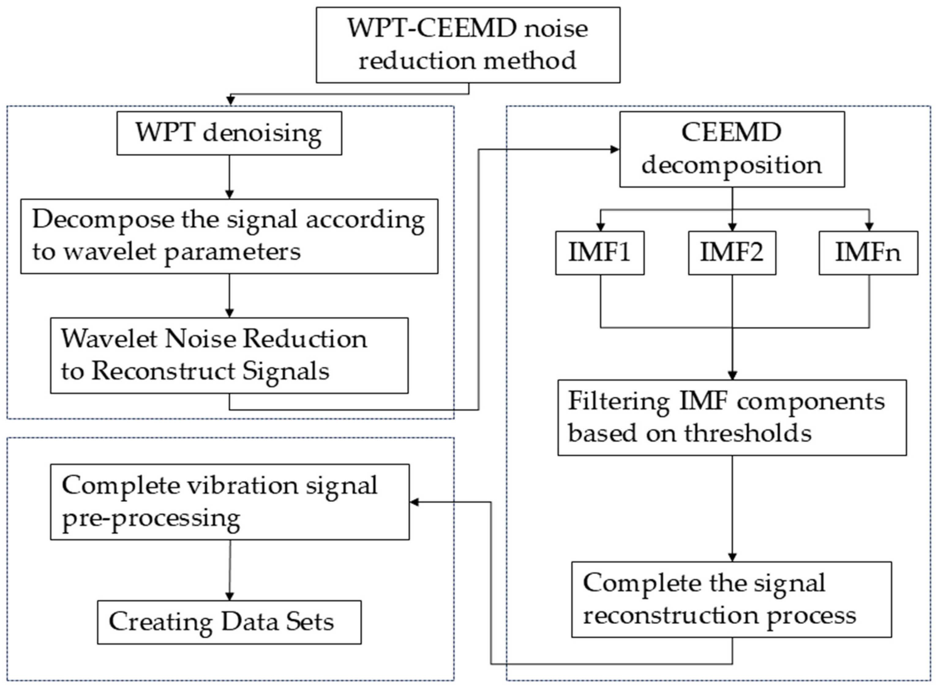
This paper proposes a dual noise reduction method that combines WPT and CEEMD to enhance the accuracy and robustness of the fault feature extraction [25,26,27]. Initially, the collected bearing fault data are processed using WPT, which enables the accurate extraction of fault feature information across different frequency bands and improves the signal’s time–frequency resolution through multiscale decomposition. Subsequently, CEEMD is applied to the processed data, utilizing an adaptive noise-assisted decomposition technique to enhance the stability of the signal decomposition. This ensures that the extracted feature components are purer and exhibit higher separability. Irrelevant noise components are eliminated by decomposing the signal into 10 IMFs and reconstructing the signal based on the correlation coefficient screening principle. By combining the strengths of both WPT and CEEMD, this method effectively removes noise interference, preserves critical fault features, and constructs a more representative dataset, thereby improving the model’s generalization capability and diagnostic accuracy. The specific implementation process is illustrated in Figure 1.
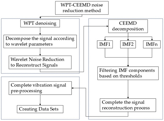
Figure 1.
WPT-CEEMD noise reduction flowchart.
2.4. CNN
CNNs process input data through multiple layers, typically consisting of an input layer, convolutional layers, pooling layers, fully connected layers, and an output layer [28,29]. Initially, the input layer receives raw data (e.g., images or signals), which are then processed by the convolutional layer to extract local features through convolutional operations, generating a feature map. The pooling layer follows, performing downsampling on the feature map to reduce both the dimensionality of the data and the computational load, while preserving the key features. Afterward, the feature map is flattened and passed to the fully connected layer, where a linear transformation is applied to map the extracted features to the output space. Finally, the output layer produces the prediction results based on the task requirements, often using an activation function for classification tasks. Through this hierarchical structure, CNNs can automatically learn and extract meaningful features from the input data, optimize the model performance via end-to-end training, and achieve strong performance in various complex pattern recognition tasks. The CNN model architecture is shown in Figure 2.
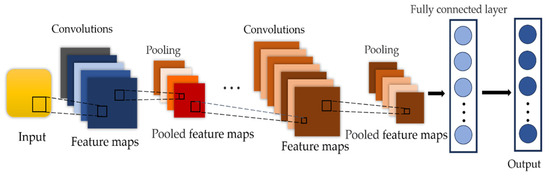
Figure 2.
CNN network structure.
2.4.1. Convolution
The convolutional layer extracts the local features of the input data through convolutional operations and passes these features to the next layer to progressively build more complex high-level features [30]. The convolution operation formula can be expressed as Equation (9), as follows:
where is the convolution kernel for feature extraction; is the input data; is the output feature map. After the convolution operation, the network can extract really different features from the input data.
2.4.2. Pooling
The pooling layer reduces the feature map size, reduces the computational effort, and improves the translation invariance of the model (which is not affected by small translations) [31].
2.4.3. Activation Function
The activation function introduces a nonlinear function that enables the model to learn complex features to better fit nonlinear data. The common activation functions are ReLU, ELU, TanH, etc. ReLU is a common nonlinear activation function, which is expressed as follows through Equation (10):
ReLU is a nonlinear activation function, which can make the neural network more nonlinear and improve the network training speed.
2.4.4. Fully Connected Layer
The fully connected layer maps the previously extracted features to the final classification or regression task. Each neuron is connected to all neurons in the previous layer, similar to a traditional neural network.
CNNs typically employ cross-entropy loss functions (e.g., Softmax and sigmoid) for classification tasks. In contrast, the sigmoid function is more suitable for prediction tasks. The sigmoid function expression is shown in Equation (11) [32], as follows:
Briefly, CNNs use a convolutional layer to extract high-dimensional features, a pooling layer to reduce the dimensionality, an activation function to introduce a nonlinear mapping, and a fully connected layer to combine and map the extracted features to the final output type [33,34]. This architecture allows CNNs to automatically learn features that are suitable for a set task and to efficiently process large-scale datasets.
2.5. LSTM
LSTM is a specialized type of recurrent neural network (RNN) designed to effectively capture long-term dependencies in sequential data. Its architecture comprises the following three key gating mechanisms: the forget gate, input gate, and output gate, which dynamically regulate information flow [35,36]. The forget gate determines which historical information should be discarded by analyzing the current input and the previous hidden state. The input gate selectively updates the cell state, ensuring that only relevant information is retained. The output gate applies a nonlinear transformation to the updated cell state to generate the current hidden state output. These gating mechanisms enable LSTM to mitigate the vanishing gradient problem inherent in traditional RNNs, enhancing its ability to model long-range dependencies. As a result, LSTM excels in tasks such as time-series forecasting, speech recognition, and natural language processing, making it a widely adopted model for applications that demand efficient and reliable sequential data processing.
The basic unit of LSTM is cell and its structure is shown in Figure 3 [37].
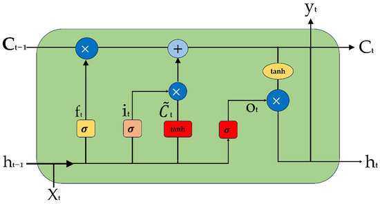
Figure 3.
LSTM basic unit.
Individual LSTM cells collaborate with memory cells through gated mechanisms to regulate the flow and storage of information, enabling the network to effectively manage and leverage past memories [38,39].
2.5.1. Forget Gate
The forget gate is mainly used to control whether past information needs to be retained or forgotten, i.e., how much historical information in the pre-cellular state can be retained to optimize the LSTM’s ability to learn long-term dependent information. The calculation formula is as follows:
where is the oblivious gate output in the range [0, 1]; and are the trainable weights and biases; is the hidden state at the previous moment, and is the current input; is the sigmoid activation function, degraded and compressed to (0, 1). If is close to 1, the past information is kept, and if is close to 0, the past information is discarded.
2.5.2. Input Gate
The input gate is responsible for deciding whether the current input information should be added to the memory cell state. The central role is to selectively introduce new information. Its formula is shown below:
where is the output of the input gate, ranging between 0 and 1, indicating the degree of incorporation of new information; and are the trainable weights and biases of the input gates; is the hidden state (short-term memory) of the previous moment; is the current input data; compresses the output values of the input gates to a value between (0, 1) in order to decide whether or not the new information enters the memory cell; is the state of the candidate cell, which indicates whether or not the new information is computed, which is jointly determined by and .
2.5.3. Updating of Memory Units
The update memory cell is used to update the contents of the cell state . The calculation formula is shown below:
where controls the introduction of new information; is a candidate cell state indicating new information for the current time step; is the final updated cell state. If approximates 1, more new information is introduced. If is approximately 0, the new information is ignored.
2.5.4. Output Gate
In an LSTM network, the output gate determines how the hidden state h at the current moment extracts information from the cell state c and outputs it by selectively outputting the information in the memory cell for the next computation or final prediction. The calculation formula is shown below:
where represents the output of the output gate; represents the weight moment of the output gate; represents the hidden state of the current time step; represents the bias term of the output gate.
LSTM accurately controls information flow through gating mechanisms, avoids irrelevant interference, stabilizes gradient propagation, reinforces time-dependent learning, and supports deeper network training.
2.6. CNN-LSTM Bearing Fault Diagnosis Algorithm Based on Double Noise Reduction
In this paper, we propose a CNN-LSTM bearing fault diagnosis method integrating WPT and CEEMD, including the following two modules: data noise reduction preprocessing and CNN-LSTM diagnosis.
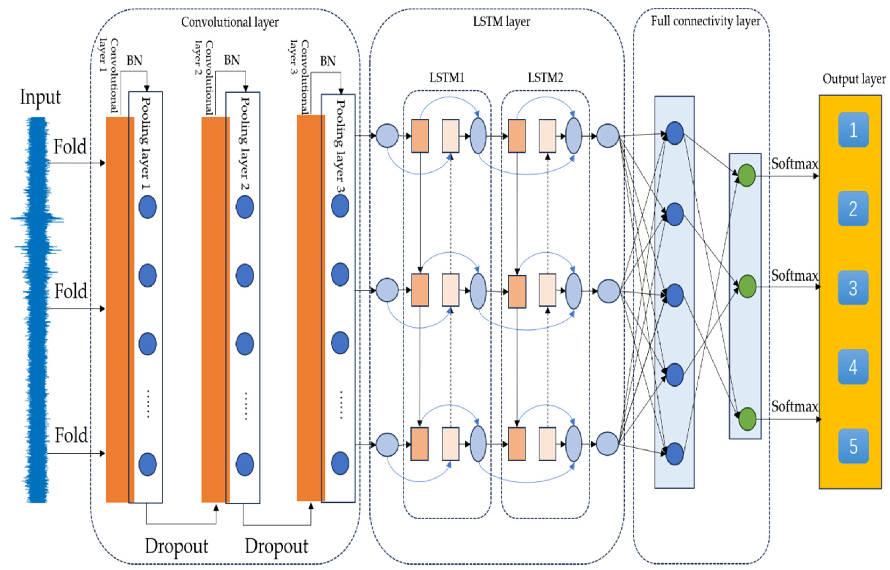
The construction of the CNN-LSTM network includes feature extraction, time-varying learning, and classification decision. Firstly, the data are processed with noise reduction using WPT and CEEMD to improve the signal-to-noise ratio. Then, the CNN extracts local spatio-temporal features and learns bearing fault patterns through convolutional and pooling layers. The CNN-extracted features are then fed into LSTM to capture temporal dependencies and enhance the fault detection. Finally, the fully connected layer is normalized using Softmax to achieve bearing fault classification. Through optimized training, the model can accurately identify fault types and improve the diagnostic accuracy. Figure 4 shows the structure of the proposed CNN-LSTM network. Table 1 shows the neural network structure parameter configurations and learnable parameter variations.

Figure 4.
Diagram of the bearing fault diagnosis process based on the CNN-LSTM neural network.

Table 1.
CNN-LSTM neural network parameter setting table.
3. Experimental Verification
3.1. Design of the Experiment
In this experiment, the rotor motor was tested under controlled laboratory conditions with constant temperature, pressure, and no external load. Fault signals were collected to facilitate the fault characteristic analysis and signal processing. The rotor motor is equipped with the following two rolling bearings: a front bearing and a rear bearing. This study specifically focuses on simulating implanted faults in the rear bearing.
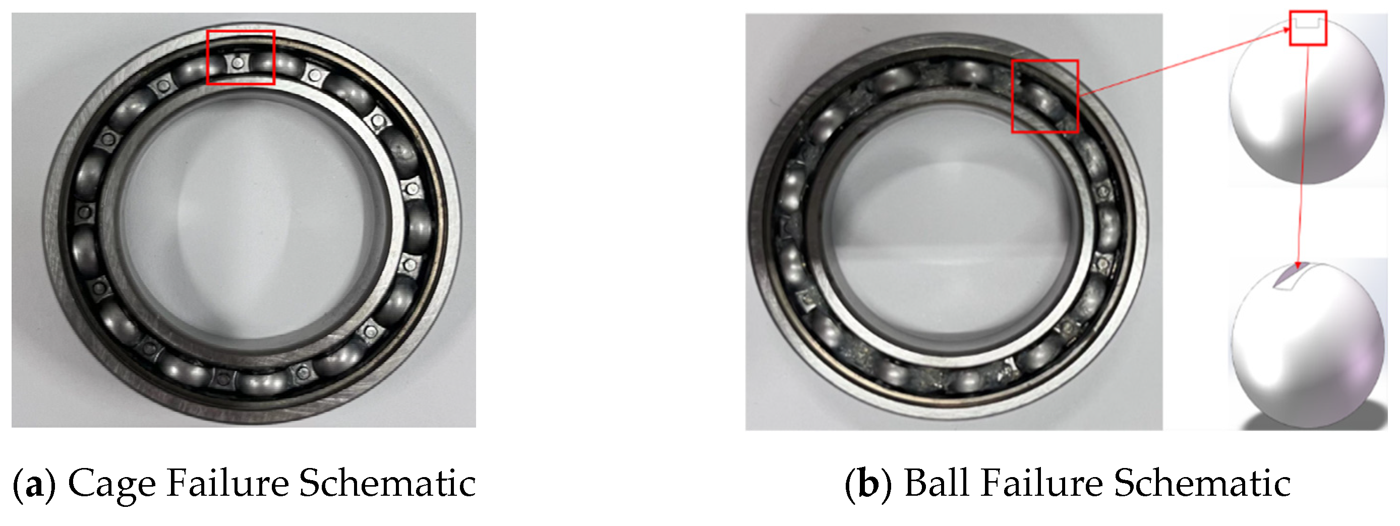
The rolling bearing used in the test is the NSK 6907 deep groove ball bearing (Nippon Seiko Corporation (NSK), Tokyo, Japan). Two fault severity levels—minor and severe—were introduced by implanting defects in the ball and cage components of the bearing to simulate different fault conditions. The precise location of the faulty bearing is illustrated in Figure 5.
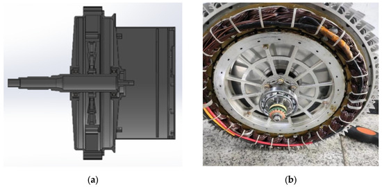
Figure 5.
Rotor bearing distribution of the wing motor. (a) rotor motor cutaway view. (b) Faulty bearing location diagram.
The main test equipment comprises hardware and software configurations, including hardware components (such as various types of sensors, host systems, data acquisition processors, and industrial power supplies) and software systems (including data acquisition software, data management software, middleware communication software, alarm management software, and stand-alone client software). The test platform’s workflow begins by regulating the rotor motor’s rotational speed through LabVIEW software version 2024 Q1. Upon receiving the command, the motor starts running. Subsequently, the vibration acceleration sensor collects real-time vibration data generated by the motor’s rotor, and these data are stored by the data acquisition processor. Additionally, the data acquisition processor is connected to an external computer, enabling real-time data monitoring and visualization, which facilitates the subsequent analysis. The architecture of the entire test platform is shown in Figure 6, and the detailed technical specifications of the vibration acceleration sensor and data acquisition equipment are provided in Table 2.
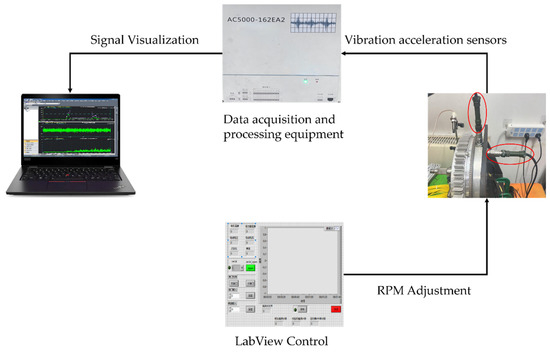
Figure 6.
Test stand architecture diagram.
Table 2.
Main equipment parameter table.
3.2. Fault Characterization Implantation
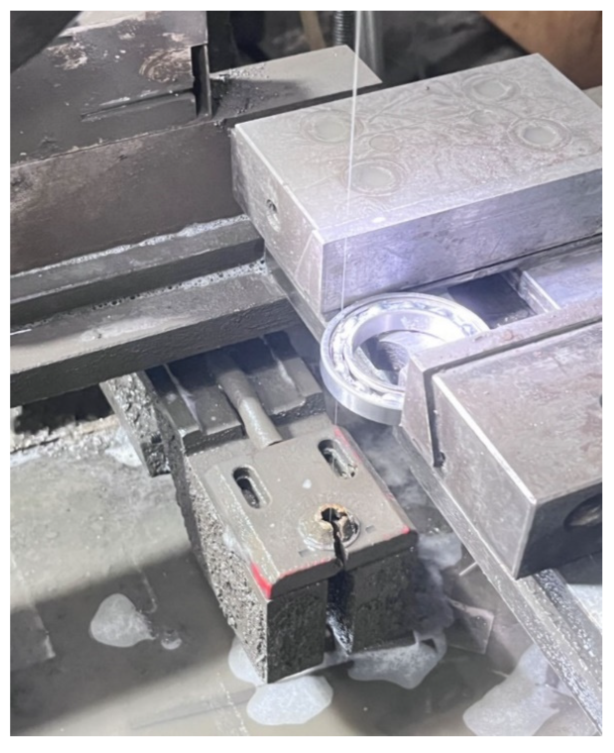
In this test, failure simulation was performed on the NSK 6907 (the bearing parameters are shown in Table 3) bearing used in the rotor motor. The failure simulation was realized by the wire cutting process to simulate the damage in actual operation. The specific fault implantation process and operation steps are shown in Figure 7. A schematic of bearing failure implantation is detailed in Figure 8.
Table 3.
NSK 6907 bearing parameters.
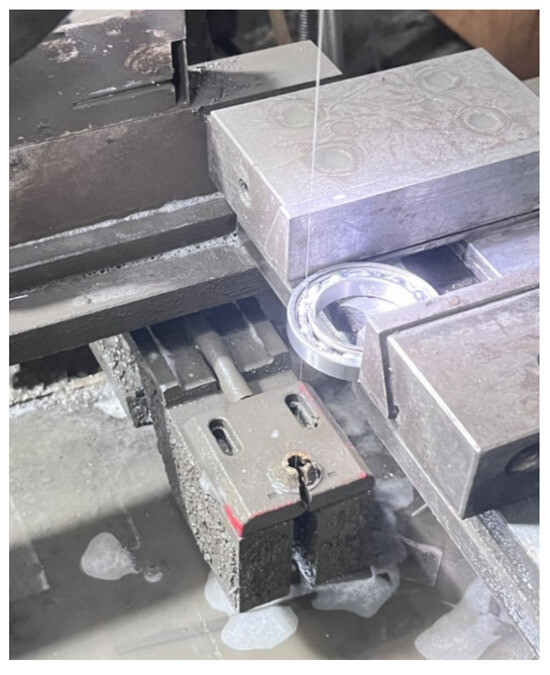
Figure 7.
Rolling bearing failure implantation process diagram.

Figure 8.
Rolling bearing failure diagram.
In order to simulate the different degrees of bearing failures, faulty bearing components with different cutting amounts were machined. The specific machining allowances are shown in Table 4.
Table 4.
Bearing failure machining allowance table.
3.3. Experimental Development
The rotor motor bearing failure simulation test enables adjustable rotational speeds ranging from 0 to 1600 RPM. Five typical speed conditions—200 RPM, 500 RPM, 800 RPM, 1200 RPM, and 1600 RPM—were established for the test. The LabVIEW system was used for precise speed control, effectively simulating various operating conditions encountered during flight.
During the experiment, the rotor motor is securely mounted on the test bench, with vibration acceleration sensors strategically placed in both the axial and radial directions to measure the rolling bearing’s vibration response along the x-axis and y-axis (as shown in Figure 9). This sensor arrangement ensures comprehensive vibration signal acquisition and high data accuracy, enabling the precise monitoring of motor vibrations under various operating conditions. This, in turn, provides a reliable data foundation for the subsequent fault diagnosis and performance analysis. The variable speed strategy employed in this test not only closely replicates the dynamic changes in working conditions during actual flight but also accurately captures the rotor’s vibration characteristics at different rotational speeds. As a result, it enables the collection of more comprehensive data, offering robust support for troubleshooting and condition monitoring.
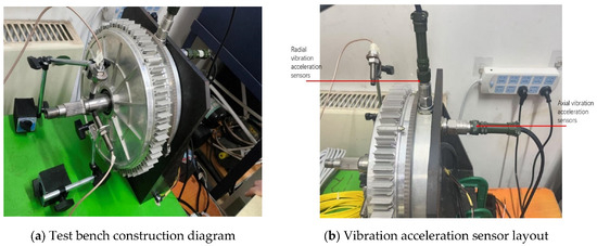
Figure 9.
Schematic diagram of the test bench as a whole.
4. Data Analysis and Processing
4.1. Vibration Signal Preprocessing for Rolling Bearings
The vibration signals of rolling bearings are an important basis for assessing the performance and health of rotor motors. However, the raw vibration signals usually contain various noise interferences, and thus require the effective preprocessing of the signals in order to extract useful fault features from them. To this end, this paper adopts a noise reduction method that combines WPT and CEEMD to preprocess the signals.
Specifically, the original vibration signal is first subjected to WPT, which captures detailed information about different frequency components through multiscale analysis, thereby enabling the effective extraction of multilevel signal features. Subsequently, CEEMD is applied to the processed signal, decomposing it into multiple IMFs, with an initial threshold set at 0.2. Regarding the IMF component selection, Xinhang Liu et al. [40] proposed a method based on the contribution value threshold criterion and, through extensive data analysis, determined an optimal threshold range between 0.5 and 0.8 for effective signal screening. Meanwhile, Haotian Wang [41], based on a large dataset, employed the energy operator ranking method to select the top four IMF components for further analysis. In this study, after thoroughly evaluating the experimental results of different fault samples at various rotational speeds, a screening criterion based on the correlation coefficient was adopted. Ultimately, a threshold of 0.2 was chosen to ensure that the selected IMF components effectively characterized the vibration signal faults.
Based on the set threshold, the IMF components with correlation coefficients ranked in the top four to five were selected to reconstruct the signal. For all data points corresponding to other fault states, the same processing method was applied to ensure consistency in the analysis process and the comparability of the results. Finally, all processed data were consolidated into a unified dataset, enhancing the stability and reliability of the data and providing more accurate and effective inputs for subsequent feature extraction, pattern recognition, and fault diagnosis.
The mathematical expression for this preprocessing process is shown below:
where denotes the original vibration signal, denotes the intrinsic modal component obtained by CEEMD decomposition, is the reconstructed signal, and the threshold is set to 0.2 to remove the noise component. Through this series of processing steps, the clarity of the signal can be significantly improved, and the vibration signal containing fault characteristics can be effectively extracted to provide more accurate data support for subsequent fault diagnosis.
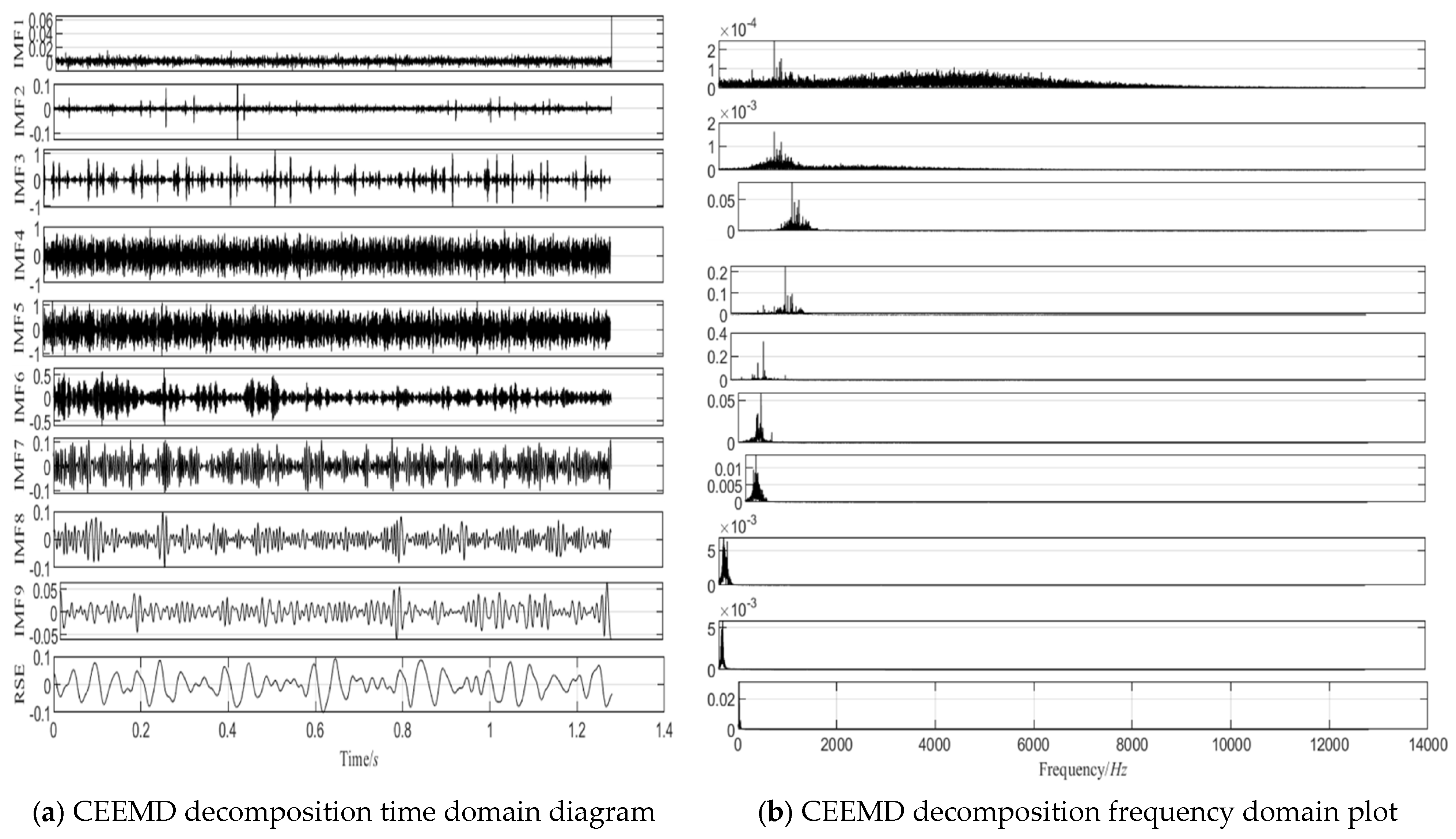
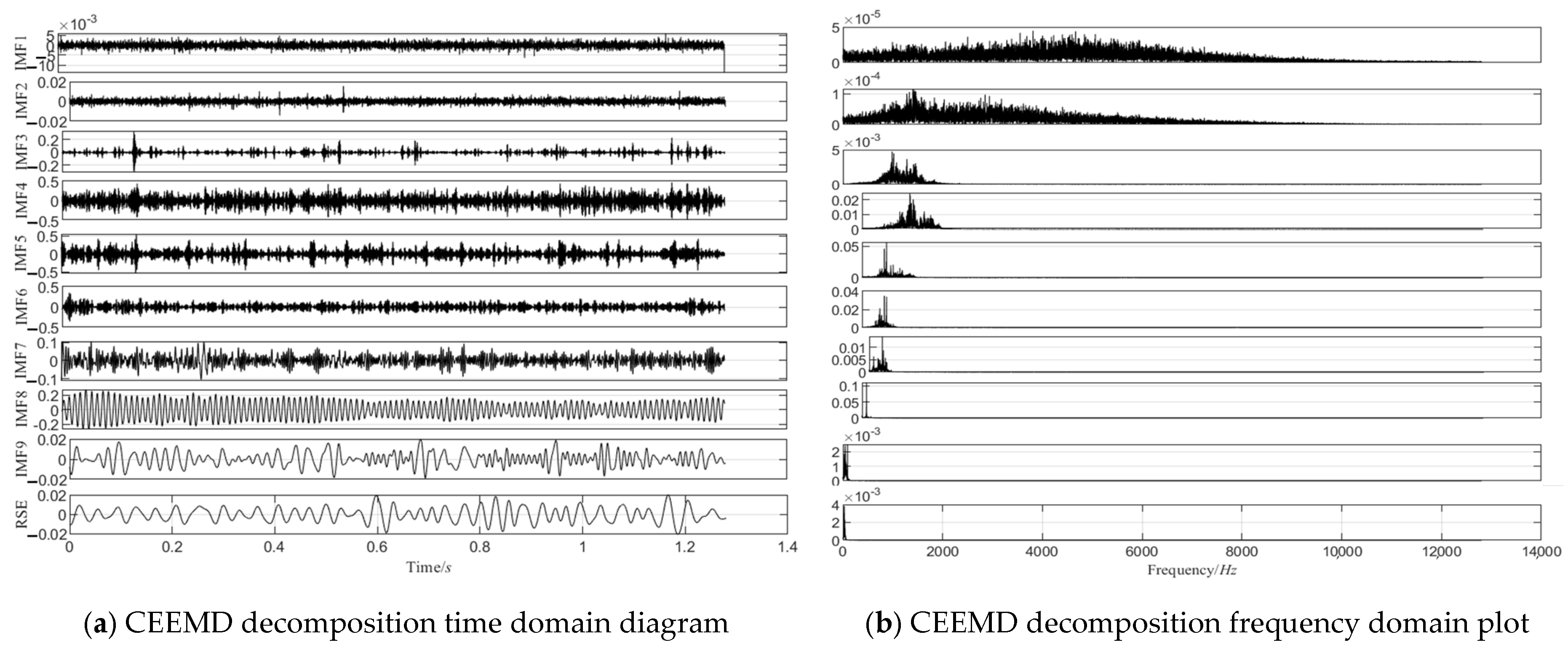
The CEEMD decomposition results at 1600 rpm, 1200 rpm, and 500 rpm are shown in Figure 10, Figure 11 and Figure 12, respectively, and the correlation coefficients of each IMF component with the original signal are shown in Figure 13.
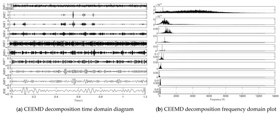
Figure 10.
The 1600 RPM CEEMD decomposition chart.

Figure 11.
The 1200 RPM CEEMD decomposition chart.

Figure 12.
The 500 RPM CEEMD decomposition chart.
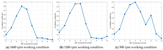
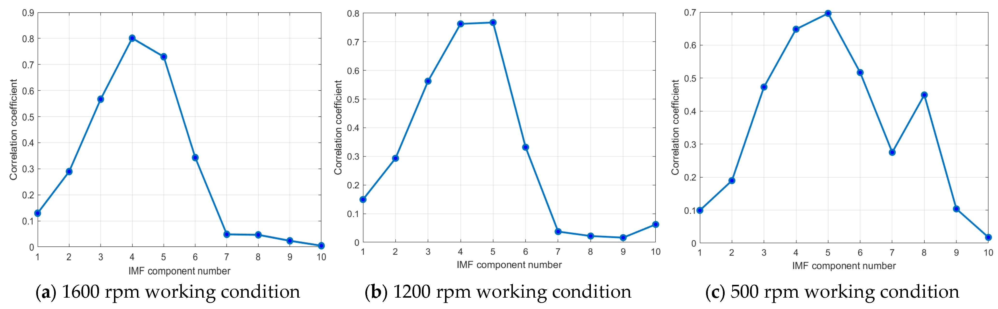
Figure 13.
Linear plot of the correlation coefficients.
As shown in Figure 13, the correlation coefficient trends of the IMF components vary significantly across the different rotational speeds. At 1600 rpm (left panel) and 1200 rpm (middle panel), the correlation coefficients increase with the IMF number, reaching their peak at the fourth or fifth IMF component before rapidly decreasing. The higher-order IMF components (e.g., Nos. 7–10) exhibit lower correlation values. This trend can be attributed to the concentration of fault-related features in the low-to-mid-order IMFs at higher rotational speeds, while high-order IMFs are more susceptible to high-frequency noise and background interference. Additionally, CEEMD prioritizes the extraction of high-frequency components, making the fault-related information the most prominent in the mid-order IMFs. Furthermore, at higher speeds, the vibration signal is more stable, with the energy more centrally distributed, leading to a rapid decline in correlation beyond the peak.
At 500 rpm (right panel), although the correlation coefficients also peak around the fourth to fifth IMF components, a notable secondary peak emerges at the eighth IMF component during the decline, a phenomenon not observed at higher speeds (1200 rpm and 1600 rpm). Several factors may contribute to this difference. First, at lower speeds, signal frequency components tend to be more concentrated in the low-frequency range, causing some higher-order IMF components to retain a significant amount of fault-related information. Second, the lower amplitude of the vibration signals increases the relative influence of the noise, leading to an altered energy distribution in the IMF decomposition. Additionally, nonlinear effects in the mechanical system—such as friction, clearance, and looseness—become more pronounced at low rotational speeds, further influencing the distribution of fault characteristics among the IMF components. Consequently, fault signals at low speeds are more susceptible to noise and nonlinear distortions. To further investigate the underlying causes of this secondary peak, a detailed analysis of the spectral and time domain characteristics of each IMF component is recommended.
In order to demonstrate the superiority of the noise reduction method proposed in this paper more intuitively, the signal-to-noise ratio (SNR) is introduced as an evaluation index in this paper [42]. Table 1 lists the comparative results of the SNR of different methods under the severe fault condition of the ball, which aims to highlight the superior performance of the proposed method in terms of noise suppression and signal fidelity. The signal-to-noise ratio is calculated as follows:
where is the power carried by the useful part of the signal; is the noise power in the signal. Table 5 shows the contrasting values of the SNR for severe ball faults.
Table 5.
SNR comparison table.
According to the SNR comparison results of different noise reduction methods in Table 5, the WPT-CEEMD method shows significant superiority. Taking the 1600 rpm working condition as an example, the SNR of the WPT-CEEMD method reaches 17.580 dB, which is significantly better than that of the WPT method (2.467 dB) and the CEEMD method (7.393 dB) alone.
Since WPT and CEEMD focus on frequency domain decomposition and modal decomposition, respectively, they are each capable of removing a certain degree of noise during processing. However, the noise reduction effect of these two methods is highly dependent on the characteristics of the signal. Specifically, for the bearing vibration signals in the experiments in this paper, especially when they contain more high-frequency noise, WPT and CEEMD may not be able to comprehensively and effectively suppress the noise when they are used individually, because their respective processing methods have certain limitations in the filtering of high-frequency noise. In contrast, by combining the advantages of Wavelet Packet Transform and CEEMD, the WPT-CEEMD method is able to fully utilize the respective advantages of both the frequency domain and modal decomposition to enhance the suppression of different types of noise. Therefore, WPT-CEEMD shows obvious advantages in the noise reduction effect, effectively improving the quality of the signal, and then enhancing the accuracy and robustness of the subsequent fault diagnosis.
4.2. Model Validation
4.2.1. Introduction to the Dataset
The test data were obtained from the test bed, with a sampling frequency of 25,600 Hz. The bearing status was categorized into the following five different categories: bearing ball single-point serious failure, bearing ball single-point slight failure, cage serious failure, cage slight failure, and normal status. The dataset contains 150 samples, with each fault type consisting of 5000 data points extracted from preprocessing at different rotational speeds, ensuring that the model can accurately assess fault categories under a wide range of operating conditions. Overall, the dataset contains 750 samples, and the sampling of each fault type follows a uniform standard, thus ensuring the consistency, balance, and representativeness of the data. The division of the training set and test set and the label setting are detailed in Table 6.
Table 6.
Rolling bearing dataset parameters.
This dataset comprehensively captures the performance of rotor motors under various flight conditions, ensuring that each bearing fault condition is adequately represented with a sufficient number of samples. The balanced distribution of fault categories enables the model to effectively learn and generalize the distinguishing features of each fault type during training. By maintaining a well-defined classification of fault types and ensuring data balance, the dataset improves the model’s reliability and accuracy in real-world applications, thus facilitating precise and consistent fault detection.
4.2.2. Model Training
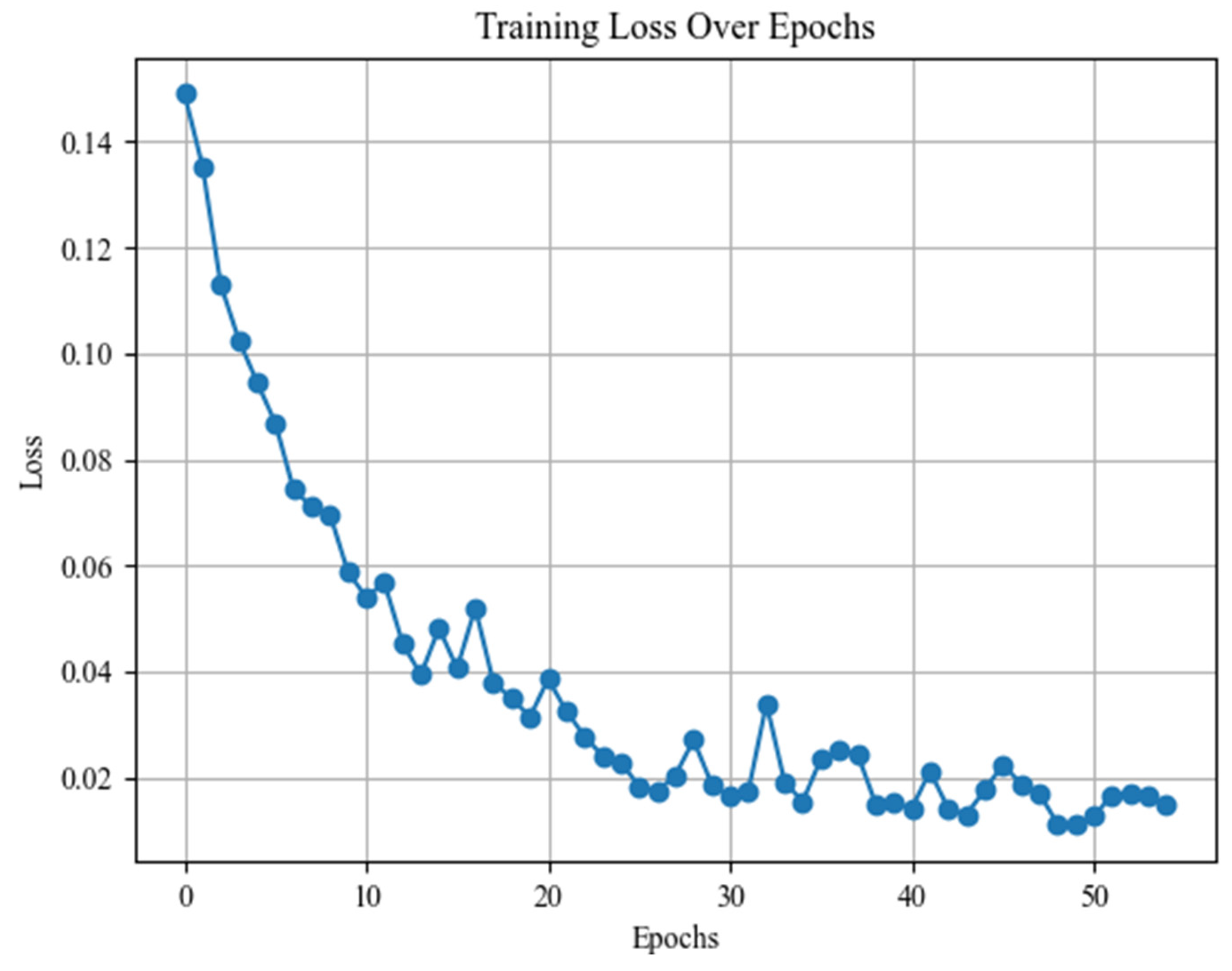
The training progress of the CNN-LSTM-based bearing fault diagnosis model is shown in Figure 14.

Figure 14.
WPT-CEEMD-CNN-LSTM model training progress chart.
The training loss of the WPT-CEEMD-CNN-LSTM model as a function of training epochs is shown in Figure 14. The training process can be divided into the following three phases: in the initial phase (0–5 epochs), the loss is high (>0.14) but decreases rapidly, indicating that the model quickly learns basic features in the early stages; during the mid-phase (5–30 epochs), the loss gradually decreases but fluctuates significantly, likely due to the model’s complexity. Additionally, while CNN extracts features, LSTM may contribute to gradient vanishing or explosion effects. In the later phase (30–50 epochs), the loss stabilizes and converges to below 0.02, indicating that the model has captured the main patterns in the data. Overall, the training curves show good performance, suggesting that the model effectively learns the data features and converges to a low training loss. Further analysis of the test loss will help assess the model’s generalization ability.
4.2.3. Comparison of Diagnostic Results and Algorithmic Analysis
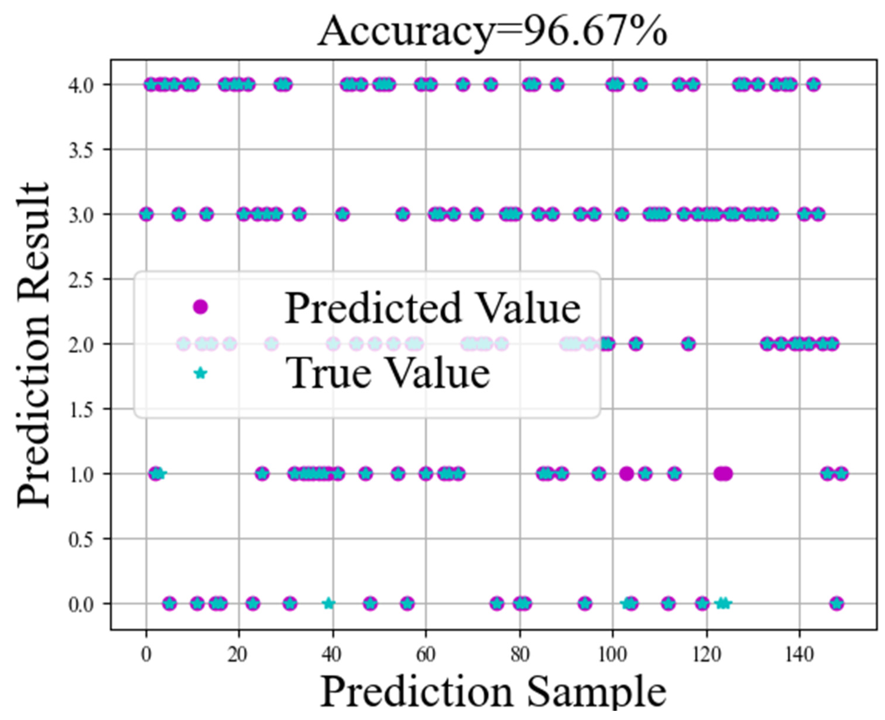
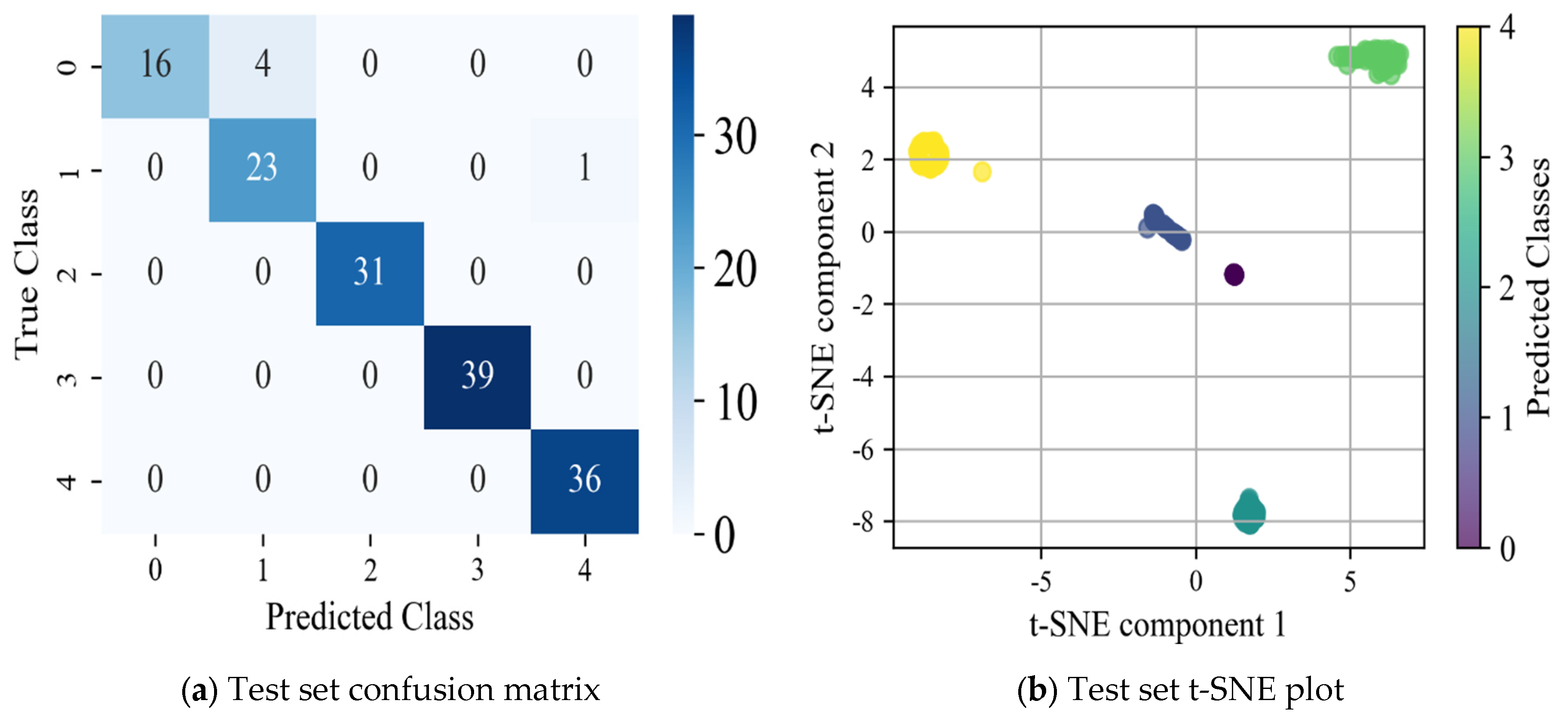
After training on the 600 sample data of the dataset, the CNN-LSTM model shows excellent prediction accuracy on the test set, as shown in Figure 15. The confusion matrix and t-SNE downscaling visualization plots for the test set are illustrated in Figure 16, offering a comprehensive evaluation of the model’s classification performance and feature distribution. The horizontal axis of the confusion matrix represents the bearing failure categories predicted by the model, i.e., the category numbers (0–4) predicted by the model, and the vertical axis represents the actual bearing failure categories, i.e., the real label numbers (0–4) of the data.

Figure 15.
Training test set result plots.

Figure 16.
Model test effect.
As shown in Figure 15, the model achieves an accuracy of 96.67% on the test set, and successfully accomplishes the task of discriminating bearings in the categories of normal state, ball faults (including both severe and slight fault states), and cage faults (including both severe and slight fault states). Through the comparative analysis of the confusion matrix and t-SNE plots, shown in Figure 16, the prediction effect and error of the model on different fault categories can be clearly observed. The confusion matrix demonstrates the relationship between the actual and predicted categories of the model, while the t-SNE plot reduces the high-dimensional features to two dimensions, visualizing the distribution of each fault category in the feature space, which can effectively reflect the model’s ability to discriminate different categories and the clustering effect. However, a certain number of samples are misidentified in the minor fault states (especially minor cage failure), which suggests that the model’s discriminative power is insufficient when dealing with minor faults. To address this issue, the Precision, Recall, and F1 Score are introduced to provide a more comprehensive evaluation of the model. These metrics help to more accurately assess the classification performance, stability, and robustness of the model [43].
- (1)
- Precision
Precision measures the proportion of samples predicted by the model to be positive that are truly in the positive category, i.e., the accuracy of the prediction, and is able to assess the model’s ability to reduce false positives, which is calculated by the following formula:
where TP is the number of samples correctly predicted as positive classes; FP is the number of samples that are actually negative classes but incorrectly predicted as positive classes. In general, a higher Precision means fewer false positives, i.e., most of the samples predicted as positive are correct.
- (2)
- Recall
Recall measures the proportion of actual positive class samples that are correctly predicted by the model, i.e., the sensitivity of the model, calculated as
where FN is the number of samples that are actually in the positive category but are incorrectly predicted to be in the negative category. A higher Recall means that the model is able to cover most of the samples in the positive category.
- (3)
- F1 Score
The F1 Score is the reconciled average of Precision and Recall, and used to strike a balance between the two, especially for cases of uneven data, and is calculated as
The higher F1 Score indicates that the model has a better balance between Precision and Recall.
Table 7 lists the key performance metrics of the WPT-CEEMD-CNN-LSTM model under each fault state, including Precision, Recall, and the F1 Score, which are used to comprehensively evaluate the model’s classification ability and stability.
Table 7.
Table of performance indicators for each failure mode model.
Table 7 demonstrates the outstanding performance of the WPT-CEEMD-CNN-LSTM model in bearing fault diagnosis. For minor ball fault detection, the model achieves an 80.00% Recall, 88.89% F1 Score, and 100.00% Precision, indicating solid classification capabilities. In detecting minor cage faults, the model performs even better, with a 95.83% Recall, 90.20% F1 Score, and 85.19% Precision, showcasing a particularly strong Recall performance. When identifying serious ball and cage faults, the model excels with a 100.00% Recall, F1 Score, and Precision, reflecting its high diagnostic accuracy. For normal state detection, the model also performs exceptionally well, achieving a 100.00% Recall, 98.63% F1 Score, and 97.30% Precision, demonstrating its ability to accurately distinguish between normal and faulty states, effectively minimizing the risk of misdiagnosis. Overall, the model’s high Recall, F1 Score, and Precision across different fault categories underscore its robustness and accuracy in fault diagnosis.
To further evaluate the diagnostic capability of the WPT-CEEMD-CNN-LSTM model on the dataset used in this study, we conducted a comparative analysis with conventional models, including CNN, LSTM, and CEEMD-CNN-LSTM. All of the models were trained and tested on the same dataset for the task of classifying and diagnosing the health condition of rotor motor bearings. To visually illustrate the classification performance of each model, Figure 17, Figure 18 and Figure 19 present the t-SNE visualizations of their respective confusion matrices and training results. Additionally, Figure 20 provides a quantitative comparison of the classification accuracies for all models after training.
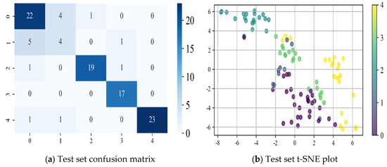
Figure 17.
CNN model.

Figure 18.
LSTM model.

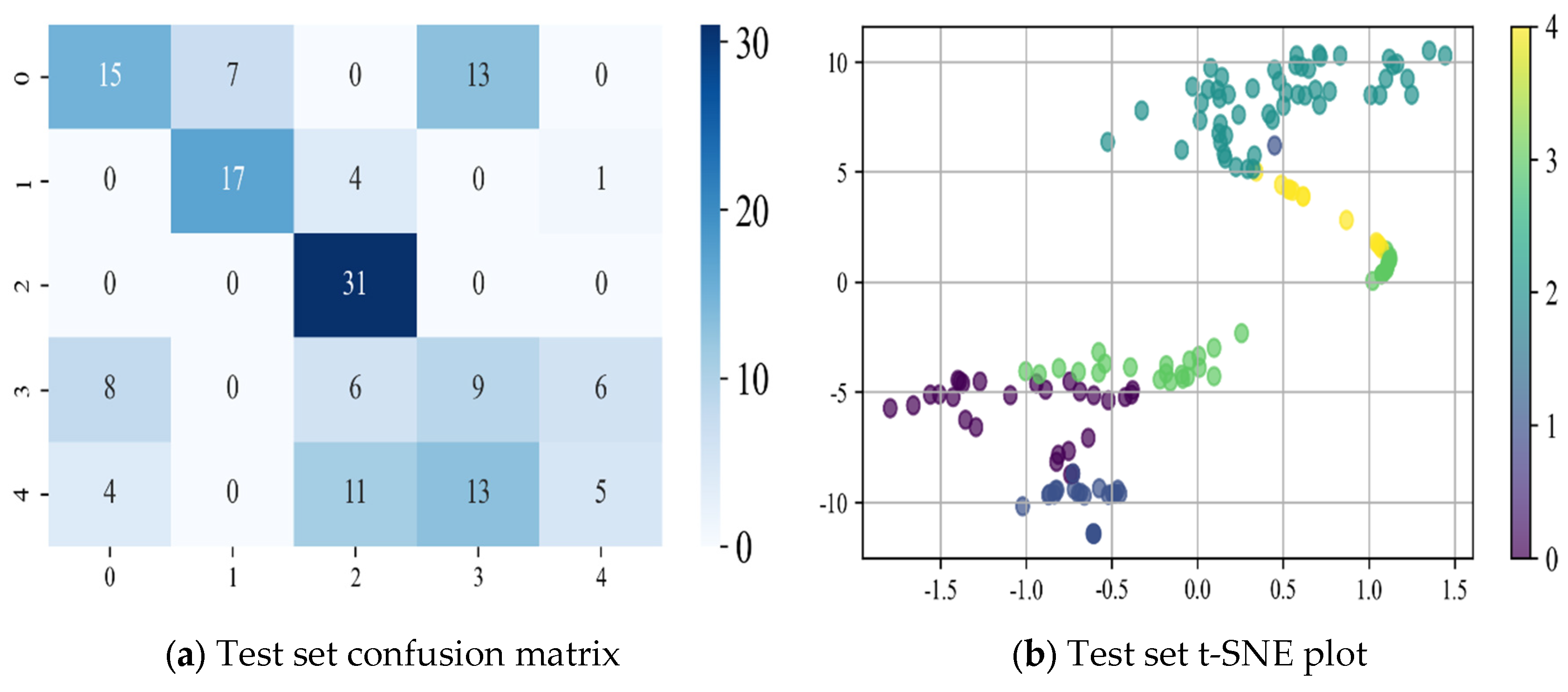
Figure 19.
CEEMD-CNN-LSTM model.
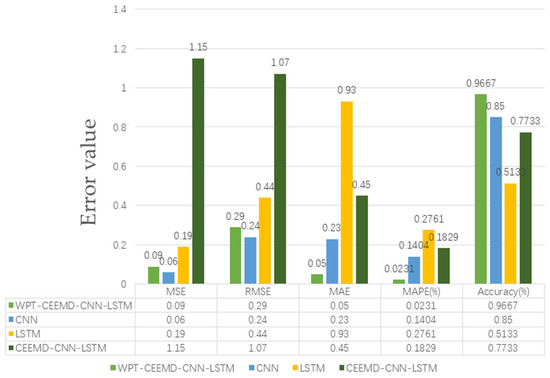
Figure 20.
Calculated results for each indicator in the test set.
Based on the confusion matrix and t-SNE dimensionality reduction results of each neural network model presented in Figure 17, Figure 18 and Figure 19, the following conclusions can be drawn:
- (1)
- The CNN model extracts local spatial features through convolutional operations and successfully performs basic classification tasks. However, its inability to model temporal information results in significant category confusion. The t-SNE visualization reveals a highly dispersed data distribution with fuzzy category boundaries, further highlighting the limitations of CNN in temporal modeling.
- (2)
- The LSTM model effectively captures temporal dependencies through its memory mechanism, resulting in improved classification performance compared to the CNN. However, the confusion matrix reveals that the misclassification rate of LSTM is not significantly reduced, and its accuracy remains lower. The t-SNE results indicate that the data clustering is tighter and the category boundaries are clearer than with the CNN, demonstrating LSTM’s advantage in handling time-series data. Nevertheless, LSTM is highly sensitive to the quality of input data and may encounter issues such as gradient vanishing or explosion during training, leading to increased computational overhead and instability in the training process.
- (3)
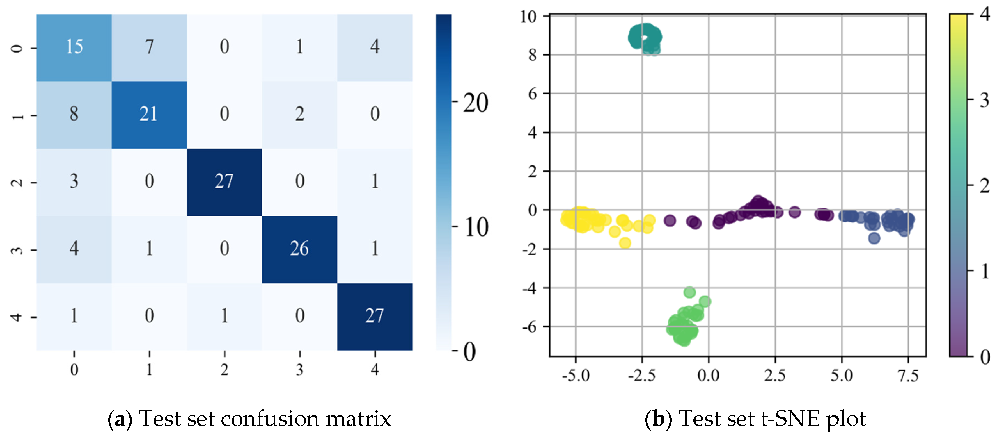
- The CEEMD-CNN-LSTM model combines the strengths of CEEMD signal decomposition, CNN spatial feature extraction, and LSTM temporal modeling, enabling it to consider both the spatial and temporal features of the data. While the model demonstrates some improvement in classification performance, as indicated by the confusion matrix and t-SNE visualization results, its accuracy is still insufficient to accurately distinguish between different fault types. Furthermore, the computational complexity of the CEEMD-CNN-LSTM model is high. The CEEMD signal decomposition process introduces additional computational overhead, and the combination of CNN and LSTM, increases the number of model parameters, leading to higher resource demands. Additionally, CEEMD signal decomposition may introduce noise, which can negatively impact both classification performance and model stability.
To more intuitively demonstrate the prediction accuracy of the proposed WPT-CEEMD-CNN-LSTM model in rolling bearing state estimation, and to comprehensively assess the overall performance of various neural network models, this paper introduces several detailed error metrics for evaluation. These include mean squared error (MSE), root mean squared error (RMSE), mean absolute error (MAE), and mean absolute percentage error (MAPE) [44,45]. These metrics provide a multi-dimensional view of the prediction error, allowing for a more comprehensive and accurate description of the model’s predictive performance.
- (1)
- MSE: The MSE is used to measure the mean squared deviation between the predicted and true values, and can reflect the degree of accumulation of the overall model error. Its calculation formula iswhere n is the number of samples, is the true value, and is the corresponding predicted value.
- (2)
- RMSE: The RMSE is the square root of the MSE, which can intuitively reflect the degree of deviation between the predicted value and the true value. Usually, the smaller the RMSE value, the higher the fit between the model’s prediction and the real value, and the smaller the overall error. Its calculation formula is
- (3)
- MAE: The MAE is used to calculate the average absolute error between the predicted value and the true value, which can intuitively measure the overall error level of the model. Usually, the smaller the MAE value, the smaller the deviation between the predicted value and the true value, and the higher the accuracy of the model. Its calculation formula is
- (4)
- MAPE: The MAPE is used to measure the percentage of prediction error relative to the true value, which can visualize the relative size of the error under different magnitudes of data. The smaller the value of the MAPE, the lower the relative error of the prediction result of the model, and the better the fitting effect. Its calculation formula is
The results of the calculation of the indicators of the test set are shown in Figure 20.
The performance of the four models (WPT-CEEMD-CNN-LSTM, CNN, LSTM, and CEEMD-CNN-LSTM) on the various error metrics (MSE, RMSE, MAE, and MAPE) and the accuracy (Accuracy%) is illustrated in Figure 20. The details are analyzed as follows:
In terms of the error metrics, the WPT-CEEMD-CNN-LSTM model achieves the best overall performance, exhibiting the lowest MSE (0.09), RMSE (0.29), MAE (0.05), and MAPE (2.31%). These results indicate that this model has the lowest prediction error and the highest accuracy. The CNN model also performs well, with relatively low error values, outperforming LSTM and CEEMD-CNN-LSTM, but still being slightly inferior to WPT-CEEMD-CNN-LSTM. In contrast, the LSTM model demonstrates weaker performance, particularly in the MAE (0.93) and MAPE (27.61%), highlighting its significant prediction bias. Among all of the models, CEEMD-CNN-LSTM exhibits the highest error values, with MSE (1.15), RMSE (1.07), MAE (0.45), and MAPE (18.29%), indicating the lowest prediction accuracy.
Overall, the WPT-CEEMD-CNN-LSTM model outperforms all of the other models across the error metrics and accuracy, demonstrating its superiority in complex data processing and time-series prediction. Its ability to achieve a high accuracy while minimizing errors highlights its robustness and reliability. These advantages make it a highly effective solution for UAV rotor motor bearing fault diagnosis, ensuring precise and efficient fault detection.
4.3. Classical Test Bed Data Validation
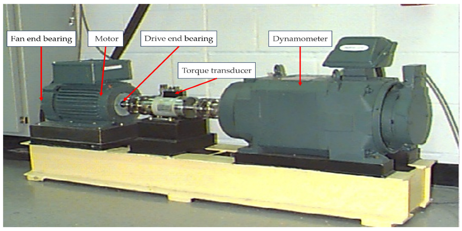
To verify the broad applicability of the method proposed in this paper for bearing fault diagnosis, rolling bearing fault data from Case Western Reserve University (CWRU), USA, were selected for analysis [46,47]. The detailed structure of the rolling bearing fault test rig is shown in Figure 21.

Figure 21.
Case Western Reserve University failed bearing simulation test bed.
The bearing failure data used in this paper was collected from a CWRU bearing test stand motor operating at 1797 rpm under unloaded conditions, with a sampling frequency of 12,000 Hz. The dataset includes the following five different operating conditions: normal operation, 0.007-inch wear failures on both the inner and outer rings, and 0.021-inch wear failures on both the inner and outer rings. To ensure data integrity and smoothness, and to accurately characterize the bearing failures, the datasets were generated following the construction methodology outlined in Section 4.2.1.
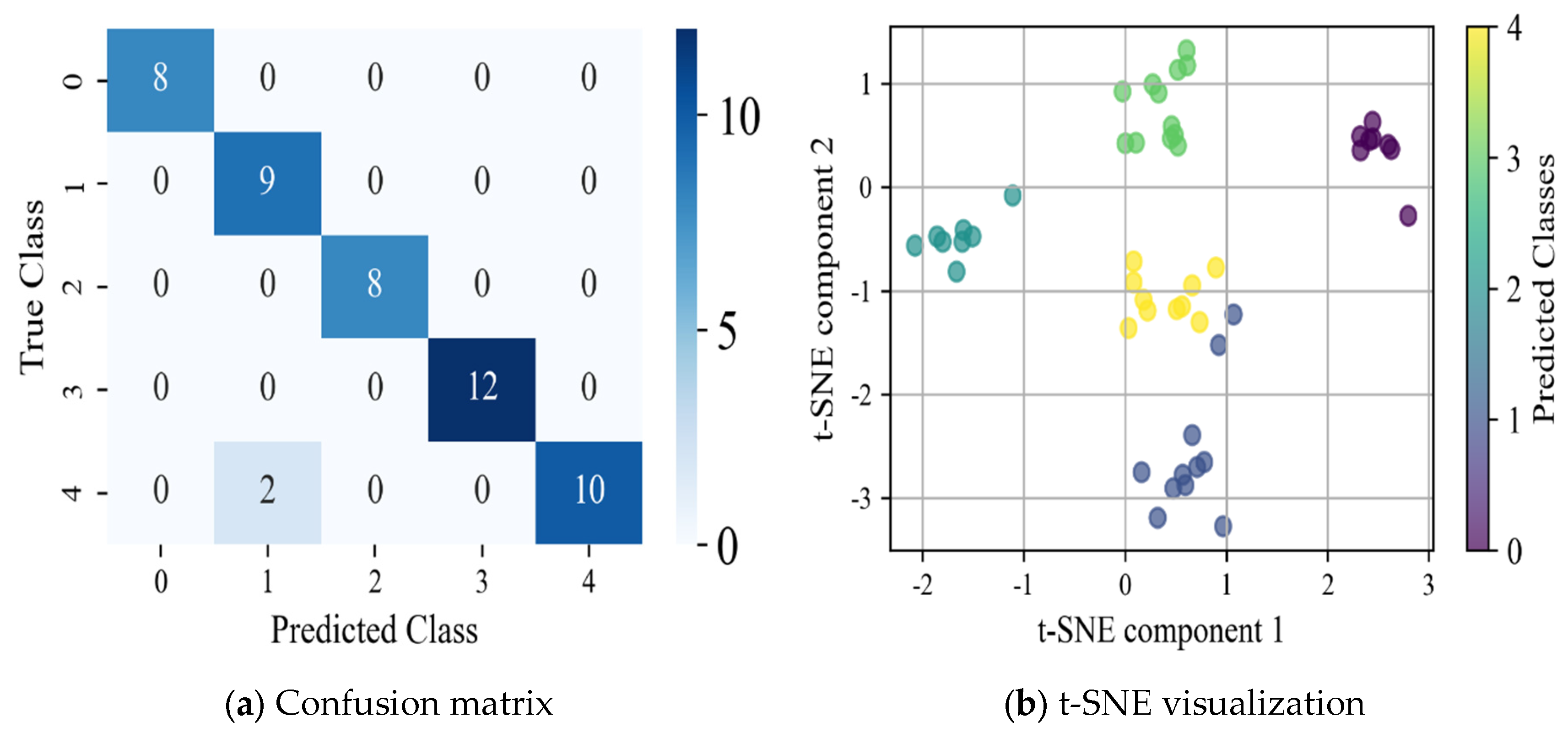
First, the raw vibration signals were preprocessed using WPT and CEEMD to effectively reduce noise and extract high-quality feature datasets. Next, a fault diagnosis model was trained on the processed dataset to enable the classification and prediction of bearing fault types. The experimental results demonstrate that the proposed method achieves high prediction accuracy in fault identification. The specific prediction accuracy is presented in Figure 22, while the confusion matrix and t-SNE visualization results for fault classification are shown in Figure 23.
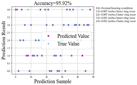
Figure 22.
CWRU faulty bearing training accuracy chart.
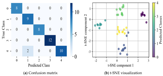
Figure 23.
CWRU bearing data training results.
The test results based on the WPT-CEEMD-CNN-LSTM model on the CWRU faulty bearing dataset demonstrate its strong performance in fault diagnosis, particularly in fault type identification and classification accuracy. The evaluation metrics—Recall, Precision, and F1 Score—effectively measure the model’s classification ability. As shown in Table 8, the model achieves a 100% Recall, Precision, and F1 Score for most fault categories, indicating exceptional classification performance. For the 0.007-inch inner ring and 0.021-inch outer ring faults, despite F1 Scores of 90.00% and 90.01%, the model maintains a high classification accuracy, with only a few misclassifications. The confusion matrix further confirms that most categories are classified with a high precision, with minimal misclassified samples, highlighting the model’s strong capability in fault recognition. Additionally, the t-SNE visualization validates the model’s ability to extract well-separated and highly distinguishable features, as evidenced by clear clustering structures. Ultimately, the model achieves an impressive 95.92% classification accuracy on the test set, demonstrating its efficiency and robustness in fault detection.
Table 8.
Model performance metrics based on the CWRU faulty bearing dataset.
According to the validation of the CWRU faulty bearing dataset and the faulty bearing dataset of the autonomous test bed, the WPT-CEEMD-CNN-LSTM model shows good scalability and adaptability, which is based on the advanced feature extraction and time-series modeling of the model, and makes it have excellent classification performance and robustness. Meanwhile, the excellent performance of the model in bearing fault diagnosis also shows certain industrial application prospects. By customizing and optimizing the model according to different industrial requirements, it can improve the fault detection accuracy in various industries and detect potential problems in time, thus significantly reducing equipment downtime. At the same time, accurate fault diagnosis can also extend the service life of equipment and reduce unnecessary maintenance costs. Therefore, the WPT-CEEMD-CNN-LSTM model not only shows excellent classification performance in UAV rotor motor bearing fault diagnosis, but also shows great potential and value in many engineering fields.
5. Conclusions
This paper focused on the fault diagnosis of UAV rotor motor bearings, specifically addressing ball and cage faults. It proposed a dual noise reduction neural network model based on WPT-CEEMD-CNN-LSTM to improve the accuracy and stability of fault identification.
In the signal preprocessing stage, the model utilized WPT-CEEMD for dual noise reduction, enabling the precise time–frequency decomposition of vibration signals while significantly improving the noise reduction performance, particularly for nonlinear and non-stationary vibration signals. Compared to traditional single noise reduction methods, WPT-CEEMD offers a notable increase in the SNR, resulting in a more stable and high-quality dataset. With this enhanced data quality, the integrated CNN-LSTM neural network model can effectively capture the evolution of bearing faults, thereby significantly improving the fault identification accuracy. The model achieved a bearing fault diagnosis accuracy of 96.67% on the test set, enabling the precise assessment of the bearing health and fully demonstrating the effectiveness and superiority of the proposed method. However, despite the model’s high overall accuracy, occasional misclassifications of individual samples still occurred, particularly for minor bearing faults. This may be attributed to the smaller amplitude of the vibration signals associated with minor faults, as well as the model’s varying sensitivity to different fault conditions, which can result in an unbalanced distribution of processed signal data. This issue underscores the need for future research to focus on enhancing the model’s sensitivity to minor faults, optimizing the dataset quality, and improving the extraction of subtle fault features to achieve more accurate assessments of rotor motor bearing fault conditions.
Overall, the WPT-CEEMD-CNN-LSTM neural network model has made significant advancements in diagnosing UAV rotor motor bearing faults, demonstrating its strong potential for application in intelligent bearing fault diagnosis. It serves as an effective fault diagnosis method, offering valuable technical support for UAV health monitoring.
Author Contributions
X.S.: Writing—original draft, Data curation, and Methodology. W.L.: Funding acquisition and Data curation. F.Y.: Data curation and Methodology. H.Z.: Methodology and Software. Z.G.: Writing—review and editing and Project administration. M.G.: Writing—original draft. B.X.: Data curation, Conducting the experiments, and Software. All authors have read and agreed to the published version of the manuscript.
Funding
This work was supported by the basic scientific research institute stability support project “WDZC-2023-ZNKZ-03”.
Data Availability Statement
The authors do not have permission to share data. The datasets presented in this article are not readily available because the data are part of an ongoing study and the product is a newly developed prototype that has not yet been officially mass-produced. Additionally, the ownership of the experimental equipment belongs to a collaborating institution, and the data are considered confidential at this stage.
Acknowledgments
This article utilizes GPT-4O to improve the neural network code and refine the text.
Conflicts of Interest
Author Min Guo was employed by the company Shanxi Diesel Engine Industry Co., Ltd. The remaining authors declare that the research was conducted in the absence of any commercial or financial relationships that could be construed as a potential conflict of interest.
References
- Wang, X.; Liu, Z.; Cong, Y.; Li, J.; Chen, H. Miniature fixed-wing UAV swarms: Review and outlook. Acta Aeronaut. Et Astronaut. Sin. 2020, 41, 023732. [Google Scholar]
- Liu, J.; Huang, D.; Wang, W. Research Progress of Unmanned Aerial Vehicle Fault Diagnosis. Control. Eng. China 2022, 29, 428–434. [Google Scholar]
- Haiyan Nie, H. Overview of rolling bearing fault diagnosis methods. Intern. Combust. Engine Parts 2019, 23, 149–150. [Google Scholar]
- Cai, Y.; Fan, Y.; Chen, W.; Zhang, J. Applications of Improved Time-frequency Analysis and Feature Fusion in Fault Diagnosis of IC Engines. China Mech. Eng. 2020, 31, 1901–1911. [Google Scholar]
- Li, C.; Chen, C. Fault Diagnosis Method of Rolling Bearing Acoustic Signals Based on ICEEMDAN. J. Shenyang Univ. Technol. 2023, 45, 672–679. [Google Scholar]
- Cui, J.; Ma, Z.; Guo, H. Application Analysis of Bearing Fault Diagnosis Based on Artificial Intelligence Technology. Mech. Eng. Autom. 2024, 6, 166–167+170. [Google Scholar]
- Huang, N.E.; Shen, Z.; Long, S.R.; Wu, M.C.; Shih, H.H.; Zheng, Q.; Yen, N.C.; Tung, C.C.; Liu, H.H. The empirical mode decomposition and the Hilbert spectrum for nonlinear and non-stationary time series analysis. Proc. R. Soc. Lond. Ser. A Math. Phys. Eng. Sci. 1998, 454, 903–995. [Google Scholar]
- Tian, J.; Wang, Y.J.; Wang, Z.; Ai, Y.; Sun, D. Fault diagnosis for rolling bearing based on EEMD and spatial correlation denoising. Chin. J. Sci. Instrum. 2018, 39, 144–151. [Google Scholar]
- Dalei, S.; Hongli, G.; Kesi, L. Adaptive De-noising Method of Mechanical Seal Acoustic Emission Signal Based on CEEMD and Wavelet Threshold. Lubr. Eng. 2019, 44, 131–137. [Google Scholar]
- Gao, S.; Li, T.; Zhang, Y.; Pei, Z. Fault diagnosis method of rolling bearings based on adaptive modified CEEMD and 1DCNN model. ISA Trans. 2023, 140, 309–330. [Google Scholar]
- Xiao, Y.; Zeng, Z.; Deng, Z.; Lin, C.; Xie, Z. An Integrated Approach Fusing CEEMD Energy Entropy and Sparrow Search Algorithm-Based PNN for Fault Diagnosis of Rolling Bearings. Comput. Intell. Neurosci. 2022, 2022, 4835157. [Google Scholar] [CrossRef] [PubMed]
- Zhang, Z.; Zhou, F.; Chen, D. Application of improved parallel LSTM in bearing fault diagnosis. In Proceedings of the 2019 Chinese Automation Congress (CAC), Hangzhou, China, 22–24 November 2019. [Google Scholar]
- Xu, M.; Yu, Q.; Chen, S.; Lin, J. Rolling Bearing Fault Diagnosis Based on CNN-LSTM with FFT and SVD. Information 2024, 15, 399. [Google Scholar] [CrossRef]
- Sahu, D.; Dewangan, R.K.; Matharu, S.P.S. Hybrid CNN-LSTM model for fault diagnosis of rolling element bearings with operational defects. Int. J. Interact. Des. Manuf. (IJIDeM) 2024, 1–12, prepublish. [Google Scholar]
- Han, K.; Wang, W.; Guo, J. Research on a Bearing Fault Diagnosis Method Based on a CNN-LSTM-GRU Model. Machines 2024, 12, 927. [Google Scholar] [CrossRef]
- Lee, D.; Choo, H.; Jeong, J. GCN-Based LSTM Autoencoder with Self-Attention for Bearing Fault Diagnosis. Sensors 2024, 15, 4855. [Google Scholar] [CrossRef]
- Xie, S.; Li, Y.; Tan, H. Fault Identification Method of Bearings Based on Improved CEEMD-SVM and Its Application. J. Railw. Sci. Eng. 2023, 20, 3192–3202. [Google Scholar] [CrossRef]
- Li, X.; Li, Y.; Cao, Y.; Wang, X.; Duan, S.; Zhao, Z. Research on Fault Diagnosis Algorithm of Aircraft EHA Based on CNN-SVM. J. Northwestern Polytech. Univ. 2023, 41, 230–240. [Google Scholar]
- Zhao, Y.; Le, Y.; Huang, J.; Wang, J.; Liu, C.; Liu, B. CEEMD and wavelet transform joint de-noising method. Prog. Geophys. 2015, 30, 2870–2877. [Google Scholar]
- Wu, T.; Jiang, D.; Wu, J.D.; Ma, J. Research on fault diagnosis of rolling bearing based on CEEMD and FastICA. J. Electron. Meas. Instrum. 2019, 33, 186–194. [Google Scholar]
- Gong, Y.; Tong, L.; Yu, Z.; Zhang, X. Research on misalignment fault diagnosis method of rotating machinery based on Pearson’s correlation coefficient. New Technol. New Prod. China 2022, 5, 48–50. [Google Scholar]
- Xiao, Y.; Li, Y.; Wang, H.; Chang, M. Feature Selection Method for Rolling Bearing in Mixed Domain Based on Pearson Correlation Coefficient. Control Instrum. Chem. Ind. 2022, 49, 308–315. [Google Scholar]
- Xiong, X. Rolling Bearing Fault Diagnosis Based on Wavelet Packet Decomposition and Hilbert Yellow Transform. Doctoral Dissertation, University of Science and Technology of China, Hefei, China, 2014. [Google Scholar]
- Li, S.; Liu, L. The study of denoising through wavelet shrinkage. Chin. J. Sci. Instrum. 2002, S2, 478–479. [Google Scholar]
- Ding, J.; Hu, J.; Lin, F. Fault Feature Enhancement Method for Rolling Bearing Based on WPT-FWEO. Mach. Tool Hydraul. 2020, 48, 194. [Google Scholar]
- Si, Y.; Guo, R.; Shi, P. Comparative Study of Signal Time-Frequency Analysis Techniques Based on EMD, EEMD and CEEMD. CT Theory Appl. 2019, 28, 417–426. [Google Scholar]
- Yang, G.; Zhong, B.; Huang, R.; Jia, M.; Xu, Y. Research on time domain feature extraction method for wavelet packet decomposition of mechanical failure signals. J. Vib. Shock. 2001, 20, 27–30+3+94. [Google Scholar] [CrossRef]
- Biao, T.; Zhousuo, Z.; Xiang, L. A Gear Fault Diagnosis Method Based on Improved Convolutional Neural Network. J. Mach. Des. 2024, 41, 1–7. [Google Scholar] [CrossRef]
- Chen, Y.; Qu, J.; Wang, X. Rolling bearing fault diagnosis method with enhanced temporal memory CNN-LSTM. Noise Vib. Control. 2025, 45, 105–111. [Google Scholar]
- Lei, J.; Jiang, Z.; Gao, Z.; Zhang, W.; Xin, B. A state estimation method based on CNN-LSTM for ball screw. Meas. Control 2024, 57, 1417–1434. [Google Scholar]
- Chen, W.; Yang, J. Illegal network identification optimization based on convolutional neural network. In Proceedings of the 2018 International Conference on Network, Communication, Computer Engineering (NCCE 2018), Chongqing, China, 26–27 May 2018. [Google Scholar]
- Jiang, A.B.; Wang, W.W. Research on optimization of ReLU activation function. Transducer Microsyst. Technol. 2018, 37, 50–52. [Google Scholar]
- Chen, Y.; Qu, J.; Wang, X.; Wang, Y. Fault Diagnosis Method of Rolling Bearings Based on CNN-LSTM with Enhanced Temporal Memory. Noise Vib. Control 2025, 45, 105–111. [Google Scholar]
- Du, Y.; Cao, Y.; Wang, H.; Li, G. A Rolling Bearing Fault Diagnosis Method Combining MSSSA-VMD with the Parallel Network of GASF-CNN and BiLSTM. Lubricants 2024, 12, 452. [Google Scholar] [CrossRef]
- Zhou, Y.; Wu, S.; Xing, W. Fault Diagnosis of Gearbox Based on Feature Fusion. Noise Vib. Control 2025, 2, 63–69. Available online: http://kns.cnki.net/kcms/detail/31.1346.TB.20250210.1336.022.html (accessed on 19 February 2025).
- Li, X.; Su, K.; He, Q.; Wang, X.; Xie, Z. Research on Fault Diagnosis of Highway Bi-LSTM Based on Attention Mechanism. Eksploat. I Niezawodn.–Maint. Reliab. 2023, 25, 162937. [Google Scholar]
- Zhang, K.; Liu, R. LSTM-based multi-task method for remaining useful life prediction under corrupted sensor data. Machines 2023, 11, 341. [Google Scholar] [CrossRef]
- Huang, K.; Zhu, L.; Ren, Z.; Lin, T.; Zeng, L.; Wan, J.; Zhu, Y. An Improved Fault Diagnosis Method for Rolling Bearings Based on 1DCNN Considering Noise and Working Condition Interference. Machines 2024, 12, 383. [Google Scholar] [CrossRef]
- Li, W.; Wang, X. Time series prediction method based on simplified LSTM neural network. J. Beijing Univ. Technol. 2021, 47, 480–488. [Google Scholar]
- Liu, X.; Luan, X.; Zhao, J.; Xiao, B.; Sha, Y. Feature Extraction Method for Rolling Bearings in Aero-Engine Based on Comprehensive Dynamic Screening. J. Aerosp. Power 2025, 1–12. [Google Scholar] [CrossRef]
- Wang, H. Fault Diagnosis of Rolling Bearings Based on CEEMD Energy Operator and XGBoost. Technol. Mark. 2023, 30, 19–22. [Google Scholar]
- Mohiuddin, M.; Islam, M.S.; Islam, S.; Miah, M.S.; Niu, M.B. Intelligent fault diagnosis of rolling element bearings based on modified AlexNet. Sensors 2023, 23, 7764. [Google Scholar] [CrossRef]
- Zhuang, Z.; Lv, H.; Xu, J.; Huang, Z.; Qin, W. A deep learning method for bearing fault diagnosis through stacked residual dilated convolutions. Appl. Sci. 2019, 9, 1823. [Google Scholar] [CrossRef]
- Zhu, H.; Huang, Z.; Lu, B.; Zhou, C. Bearing remaining useful life prediction of fatigue degradation process based on dynamic feature construction. Int. J. Fatigue 2022, 164, 107169. [Google Scholar]
- Chicco, D.; Warrens, M.J.; Jurman, G. The coefficient of determination R-squared is more informative than SMAPE, MAE, MAPE, MSE and RMSE in regression analysis evaluation. PeerJ Comput. Sci. 2021, 7, e623. [Google Scholar] [CrossRef] [PubMed]
- Jiang, L.; Gao, M.; Li, H. Fault identification method for bearings based on dual-channel CNN using SSA-VMD and SDP. J. Mech. Electr. Eng. 2025, 42, 257–266. [Google Scholar]
- Yu, N.; Wei, C.; Tian, L.; Zhao, J.; Yu, X. The application of mayfly optimized dual-channel network in gearbox fault diagnosis. J. Xi’an Jiaotong Univ. 2025, 5, 1–12. [Google Scholar]


Disclaimer/Publisher’s Note: The statements, opinions and data contained in all publications are solely those of the individual author(s) and contributor(s) and not of MDPI and/or the editor(s). MDPI and/or the editor(s) disclaim responsibility for any injury to people or property resulting from any ideas, methods, instructions or products referred to in the content. |
© 2025 by the authors. Licensee MDPI, Basel, Switzerland. This article is an open access article distributed under the terms and conditions of the Creative Commons Attribution (CC BY) license (https://creativecommons.org/licenses/by/4.0/).