Abstract
Hard turning is a precision machining process used in the manufacturing industry for the finishing of hardened alloy steel, which is known for its high hardness and wear resistance. In this work, an experimental investigation was conducted to predict surface roughness and cutting temperature during the hard turning of AISI 52100 steel using the minimal cutting fluid application (MCFA). The MCFA is a sustainable high-velocity pulsed jet technique that has emerged as an eco-friendly approach for reducing the environmental impact and improving surface integrity in machining processes. The influence of key machining parameters, such as cutting speed, feed rate, and depth of cut, on the performance indicators was modeled using the response surface methodology (RSM) and the artificial neural network (ANN). The RSM was employed for a structured, statistical analysis, while an ANN provided a data-driven approach for capturing complex non-linear relationships. Various network architectures were established and evaluated with a fixed number of cycles. Results showed that the ANN exhibited superior accuracy in predicting both responses. In comparison to the QR model, the ANN exhibited the lowest average error rate in accurately predicting the response. This was further validated through experimental trials, demonstrating that the ANN consistently outperformed the RSM across different parameter settings. Additionally, the use of the MCFA contributed to sustainable manufacturing by minimizing the use of cutting fluids while maintaining machining quality.
1. Introduction
The exceptional wear resistance and compressive strength of hardened steels make them a preferred choice for manufacturing heavy machinery components, tools, and automobile parts. Astakhov [1] reported that hard turning offers numerous benefits, including reduced setup times, fewer process steps, flexibility in part geometry, less expensive equipment, and fewer tools. To enhance surface finish and minimize tool wear, it is crucial to mitigate the cutting force, friction, and cutting temperature during the hard turning process. This process often involves flood cooling with large quantities of cutting fluid, which can lead to thermal distortions and harmful fumes from the vaporization of fluids at high temperatures, negatively impacting operator health and the environment. Although these issues can be addressed with dry machining, the various limitations of the dry hard turning process, as viewed by researchers, are higher tooling cost, needing rigid machine tools, excessive tool wear, residual tensile stress at the surface, formation of white layer, and microstructural alteration of the machined surface. In the minimal cutting fluid application (MCFA) techniques, a small amount of cutting fluid is delivered as high-velocity pulsing jets to penetrate the cutting zone more effectively than a continuous stream. This approach enhances cutting performance by improving surface finish and dimensional accuracy, reducing tool-chip contact length and tool wear while maintaining optimal cutting forces. Anand et al. [2] reported that the MCFA in hard turning significantly reduced cutting force and cutting temperature and improved tool life and surface finish, compared to dry and minimum quantity lubrication (MQL)-assisted hard turning. Specifically, the MCFA reduced cutting force by 15.85%, cutting temperature by 6.80%, and surface roughness by 23.52% during the hard turning of OHNS steel, compared to the MQL. The MCFA demonstrated superior performance compared to MQL. However, despite these advantages, its full-scale implementation and optimization across diverse machining conditions remains an area of active research. Critical aspects, such as thermal behavior, microhardness variation, and residual stress formation, remain key research areas. A deeper understanding of these factors is essential in maximizing the MCFA’s effectiveness and ensuring its broader industrial applicability. Modeling techniques are essential for optimizing machining operations, reducing manufacturing time, and cutting costs. Since machining operations are non-linear, analytical models often require simplifications and assumptions for better accuracy. Recently, Artificial Intelligence (AI) models, particularly artificial neural networks (ANNs), have gained popularity for their reliability and effectiveness in metal-cutting applications. Numerous researchers have successfully implemented ANN-based models. Özel and Karpat [3] created a model for predicting surface roughness and tool flank wear in the finish during the dry hard turning of AISI H13 steel. A backpropagation neural network was trained using experimental data on surface roughness and tool flank wear to facilitate precise predictions of machining performance. The trained model effectively predicted surface roughness and flank wear across various cutting conditions, demonstrating high predictive accuracy within the trained parameter range. Nalbant et al. [4] employed both regression analysis and an ANN model to forecast surface roughness during the CNC turning of AISI 1030 steel. A comparative evaluation between the prediction accuracy of the ANN model and the regression models was conducted. The findings revealed that the ANN model exhibited superior predictive accuracy for surface roughness compared to the multiple regression-based approach. Quiza et al. [5] developed an artificial neural network model for tool wear using a backpropagation training algorithm in the hard machining of D2 AISI tool steel. A non-linear relationship between surface roughness and the machining conditions was established, which justified the use of the ANN model. The neural network model was shown to have a better capability in making accurate predictions of tool wear under the conditions studied.
Leo Dev Wins and Varadarajan [6] developed an ANN-based model to predict surface roughness based on fluid application parameters, including injector pressure, pulsing frequency, and fluid application rate, during the hard milling of AISI 4340 steel with minimal fluid usage. Among various architectures tested, the 3-6-6-1 configuration demonstrated the lowest root mean square error (RMSE) of approximately 0.01, establishing it as the optimal model. The predictions from the ANN model closely matched experimental results, underscoring its efficacy. Chandrasekaran et al. [7] presented reviews of works related to the application of popular soft computing techniques like an ANN, fuzzy concept, genetic programming concept, simulated annealing technique, particle swarm, and ant colony concepts. Fuzzy coupled with neural network was the most efficient concept for modeling, whereas genetic programming and particle swarm concepts were the most efficient for optimization. Sethi and Kumar [8] developed a flank wear model by using the response surface methodology (RSM), which is capable of quantifying tool wear under various cutting conditions. A central composite design was employed for experimental optimization. It was determined that cutting speed emerged as the most significant parameter influencing flank wear, which was followed by depth of cut and feed rate. Aouici et al. [9] developed models for surface roughness and cutting force components by using the RSM during the hard turning of heat-treated AISI H11 steel with a Cubic Boron Nitride tool (CBN7020). Cutting force components were primarily influenced by the depth of cut and workpiece hardness, while statistically significant effects on surface roughness were attributed to both feed rate and workpiece hardness. Bouacha et al. [10] developed models for cutting force and surface roughness and optimized the process parameter through the composite desirability approach using the RSM in hard machining of AISI 52100 bearing steel by using CBN cutting tools. Surface roughness was mainly influenced by feed rate and cutting speed, whereas cutting forces were influenced by depth of cut. Attanasio et al. [11] conducted a comparative analysis between the RSM and the ANN models to investigate tool wear during the machining of AISI 1045 hard metal using tungsten carbide cutting tools. The ANN model was identified as the most effective as it yielded the lowest fitting error compared to the other models. Chinchanikar and Choudhury [12] presented a comprehensive report on the modeling of tool wear, temperature, and cutting forces during hard machining. The major techniques reported included the RSM, finite element modeling, stochastic modeling, ANN modeling, and hybrid modeling. Cica et al. [13] compared experimental results with those from developed models regarding surface roughness and tool wear during the hard machining of 100Cr6 steel (62 HRC) using coated carbide tools under high-pressure cooling conditions. Both ANNs and Adaptive Neuro-Fuzzy Inference Systems (ANFIS) were employed to develop the models for tool wear and surface roughness, demonstrating strong agreement with the experimental findings. Mia and Dhar [14] developed empirical relationships using the RSM and ANN to correlate average tool–workpiece interface temperature with cutting speed, feed rate, and workpiece hardness during the hard turning of AISI 1060 alloy steel. Both models achieved ≥99% accuracy, with the ANN model showing a mean absolute error of about 5% and a regression coefficient of over 99.9%. The ANN model demonstrated superior accuracy compared to the RSM. Panda et al. [15] developed an ANN and quadratic regression (QR) model for surface roughness and tool wear in the turning of AISI 52100 hardened alloy steel using multilayer coated carbide insert. The results obtained revealed that the ANN model gives accurate prediction of responses with minimum average error percentage when compared QR model. Labidi et al. [16] developed predictive models for arithmetic surface finish (), flank wear (), and tangential force () during the hard turning of X210Cr12 hardened steel (56 HRC) using a Coated Ceramic tool (CC6050). The ANN and RSM models demonstrated a strong correlation with the experimental data. However, the ANN approach showed better accuracy and the capability of predicting machining responses than the RSM. Zerti et al. [17] investigated the influence of machining parameters, specifically cutting speed (), depth of cut (), and feed rate (), on surface roughness indicators (, , and ) and cutting force components (, , and ) during the dry hard turning of AISI 420 (59 HRC) martensitic stainless steel. The investigation employed both the RSM and the ANN to model the machining process. The results indicated that the ANN model outperformed the RSM model in terms of accuracy and predictive capability. Kumar et al. [18] conducted an investigation into flank wear, surface roughness, and chip-tool interface temperature during the hard turning of heat-treated AISI D2 grade tool steel using indexable multilayer coated carbide inserts. Both the RSM and the ANN models were developed, and a comparative assessment between experimental and predicted results was performed. The ANN model provided more accurate predictions for flank wear compared to the RSM model, while for surface roughness and chip-tool interface temperature, the RSM-based predictions demonstrated greater accuracy than the ANN model.
Elsadek et al. [19] applied the ANN and RSM predictive tools for predicting surface roughness in the hard turning of AISI H13 hot work steel. The results showed that the RSM prediction model has an average relative error of 5.07%, while the ANN model has an average relative error of 2.21%. Adizue et al. [20] developed predictive surface roughness models for the ultra-precision hard turning of AISI D2 steel (62 HRC) using the SVM, GPR, ANFIS, and ANN machine learning algorithms. The models demonstrated excellent accuracy, achieving an average Mean Absolute Percentage Error (MAPE) of 7.38%. The MAPE values for the AN-FIS and the ANN were 9.98% and 3.43%, respectively. The validation with experimental data yielded satisfactory R, RMSE, and MAPE values of 0.78, 0.19, and 36.17%. Şahin [21] developed the RSM and ANN models to predict surface finish during the machining of AISI 1040 hardened mild steels using coated carbide tools with triangular and square geometries under varying conditions. The predictive capability of the ANN model was found to surpass that of the RSM, as evidenced by the coefficients of determination of 0.995 for the ANN and 0.925 for the RSM, which correspond to mean squared errors of 0.00056 and 0.0088, respectively. Bañon et al. [22] conducted a comparative analysis between the RSM and predictive models based on artificial neural networks ANNs during the laser texturing of S275 carbon steel alloy. The ANN-based model demonstrated exceptional accuracy, achieving prediction fits exceeding 90% for all output variables, which surpassed the performance of the RSM. The ANN model demonstrated enhanced adaptability to variations in the results obtained. An investigation on the High-Speed Turning (HST) on AISI D2 steel using a coated carbide cutting tool in dry conditions was conducted by Mebrek et al. [23]. The result revealed that cutting speed has a crucial role in determining cutting temperature, surface roughness, and flank wear. The non-linear prediction models for every measurable output were developed and tested for their efficacy with three statistical measures: R2, MAPE, and RMSE. In order to identify the optimal cutting parameters, multiobjective optimization with the Desirability Function (DF) method was employed. The optimal values for , , and were 477.28 m/min, 0.08 rev/min, and 0.8 mm, respectively, which leads to a value of 1.23 μm. Using self-driven rotary cutting tools, Bien [24] assessed models for surface roughness prediction on 40X steel shafts with a hardness of 45 HRC. The models were built using the ANN, genetic programming (GP), and Multivariable Regression Analysis (MRA). The ANN model provided the most accurate evaluation criteria, with the lowest MAPE (7.207%) and MSE (0.032) values; in contrast, the GP and MRA models had lower confidence predictive criterion values. Optimization of cutting conditions for machining titanium alloy (Ti-6Al-4V) utilizing carbide alloy inserts was investigated by Hossain et al. [25] by using the RSM. Vasconcelos et al. [26] included noise variables in their experimental design. A composite design was used to integrate controlled variables with noisy variables. The data were inputted into eight different topologies of artificial neural networks. The predictive model was more accurate and robust with the 7-20-14-1 network configuration, which had the lowest root mean square error and mean absolute error values. Surface finish models for machining AISI 1040 hardened mild steels with coated carbides utilizing two alternative geometries, triangle and square, were developed by Şahin [21]. ANNs and the RSM were used to compare the outcomes. ANNs exhibited enhanced predictive capabilities; both methods demonstrated that feed rate was crucial. The study indicated that the ANN is an excellent tool for engineering design and industrial applications due to its time efficiency and enhanced accuracy in outputs. Ambhore et al. [27]’s unique tool wear model with residual values and R2 value of 0.93 was confirmed reliable. Real-time tool acceleration underpins the model. The suggested model’s tool wear regression value was supported by an ANN. Kumar et al. [28] proposed using machine learning to predict cutting forces and surface roughness in AISI 52100 steel for marine, biomedical, and renewable energy applications. Cutting forces and surface roughness were strongly affected by depth of cut and feed rate, respectively. The study used the RSM and desirability function to optimize cutting parameters to improve surface quality and machining efficiency. Sukonna et al. [29] used the ANN, RSM, and ANFIS to analyze the machinability of medium carbon hardened steel in dry and high-pressure cooling environments, revealing accurate descriptions of machining responses using a Correlation Coefficient Factor (R), MSE, RMSE, and MAPE. In machining and manufacturing processes, the issues associated with artificial neural networks (ANNs) in predictive modeling include data dependency, overfitting, intricate parameters, and substantial computing expenses. The performance of artificial neural networks is dependent upon the quality of training data; inadequate or noisy input can diminish accuracy. Overfitting might result in inadequate generalization, whereas choosing the appropriate network architecture and hyperparameters requires knowledge. Also, artificial neural networks need a lot of computing power to be trained, which makes it hard to use them in real time in some manufacturing applications.
Hard turning induces intense heat, impacting tool wear, dimensional precision, and surface integrity, which makes precise temperature prediction crucial for process optimization. Additionally, surface roughness significantly affects the functionality and lifespan of machined components. Therefore, it was imperative to conduct predictive modeling of cutting temperature and surface roughness under MCFA conditions to enhance machining performance. Despite the successful use of the ANN for modeling various machining processes, there is limited work on modeling cutting temperature and surface roughness in the hard turning of alloy steel. This study focused on developing an ANN-based model to predict cutting temperature and surface roughness based on cutting parameters during the hard turning of AISI 52100 steel using the MCFA technique.
The objectives outlined below aimed to address this research gap:
- To create predictive models for surface roughness and cutting temperature in the hard turning of AISI 52100 steel using the RSM and the ANN.
- To evaluate the performance of the MCFA technique in comparison to dry and MQL environments during hard turning processes.
- To compare both the accuracy and reliability of the RSM and ANN models in predicting surface roughness and cutting temperature with implications for their potential use in sustainable machining practices.
2. Materials and Methods
2.1. Test Specimen and Chemical Composition
The workpiece material used in this investigation was AISI 52100 hardened alloy steel, which has a hardness of 58 HRC. In the automotive and related industries, this alloy steel has a variety of uses, including bearings, forming rolls, and spindles. The chemical composition of the AISI 52100 workpiece was tested using BRUKER’S optical emission spectrometer (Model—Q4 TASMAN). Table 1 presents the chemical composition of the workpiece determined through OES.

Table 1.
Chemical composition of AISI 52100 steel specimen in percentage by weight (OES).
2.2. Experimental Setup
A literature review [16] and the recommendation of the tool manufacturer were used to select the inserts and the tool holder. For the experiments, a MTCVD multilayer coated carbide (TiN/TiCN/Al2O3) HK150, K-type cutting insert with the specification CNMG120408, and the tool holder with PCLNR 2020 K12 specification were chosen. The combination of a cutting insert with a tool holder resulted in an included angle of 80°, a back rake angle of −6°, a negative cutting edge inclination angle of −6°, a clearance angle of 5°, an approach angle of 95°, and a nose radius of 0.8. The experiments were conducted on a high-precision HMT NH-18 lathe machine equipped with an MCFA setup, which delivered small pulses of cutting fluid. A minimal quantity of SUN Cut ECO-33, a high-performance, eco-friendly semi-synthetic cutting fluid with a pH of 9–9.2 (5% concentration), viscosity of 48 mm²/s (30 °C), specific gravity of 0.96–1.060, and a refractive index of 1.4, was used. It is free from hazardous chemicals, non-toxic, fireproof, and safe for direct sewer disposal. Cutting and cutting fluid application parameters were selected based on prior studies, with optimal settings: pressure () = 100 bar, flow rate () = 12 mL/min, pulse frequency () = 30° pulses/min, and nozzle stand-off distance of 20 mm. The experimental design followed Taguchi’s L27 Orthogonal array. Figure 1 illustrates the experimental setup for minimal cutting fluid application.
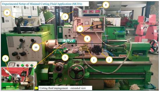
Figure 1.
Experimental setup of minimal cutting fluid application. (1) AC Motor; (2) Fluid Pump; (3) Variable Frequency Device; (4) Cutting Fluid Tank; (5) Cutting 287 Fluid High-Pressure Line; (6) Nozzle; (7) Dynamometer; (8) Digital Display unit; (9) Infrared 288 Thermometer; (10) Thermocouple Cable.
2.3. Measurement of Surface Roughness and Cutting Temperature
The surface roughness was measured using Taylor Hobson Talysurf4 surface roughness measuring machine, as shown in Figure 2. The surface roughness was measured at three locations around the workpiece circumference. The value of the surface roughness is the average of three points taken for each measurement.
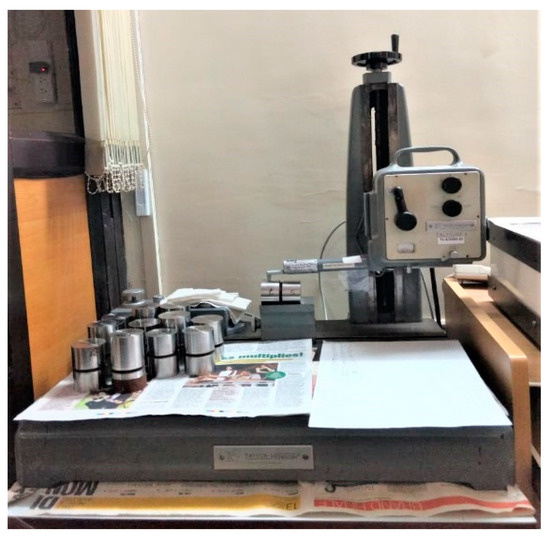
Figure 2.
Measurement of surface roughness using Talysurf4 Surface Roughness Testing Machine, Salbro Engineers, Mumbai, India.
Measuring cutting temperature presents significant challenges in metal-cutting operations. The temperature at the tool-chip interface during metal cutting is complex, making it challenging to establish a measurement setup. Therefore, the accurate measurement of temperature remains a significant challenge. In this study, an infrared thermometer and embedded thermocouple technique were used to measure the cutting temperature (cutting edge temperature), as explained by Honey et al. [30] in their research work.
Figure 3 shows the cutting tool with an embedded thermocouple. The HTC IRX-68 Infrared Thermometer measures temperature ranges from −50 °C to 1850 °C (IR) and −50 °C to 1370 °C (Type K), with accuracies of ±1.0% (IR) and ±1.5% (Type K). The primary specifications included a response time of less than 150 ms, an optical resolution of 50:1, and an adjustable emissivity ranging from 0.10 to 1.0. The K Type thermocouple probe connected to the device ensured precise and accurate temperature monitoring. The thermocouples were positioned in holes less than 0.3 mm from the cutting edge of the insert. The holes were made by Electric Discharge Machining (EDM) normal to the tool flank face; the thermocouple can be positioned as close to 0.15 mm from the cutting edge. To prevent damage, thermocouples were inserted into blind holes machined by EDM.
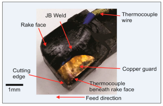
Figure 3.
Tool with embedded thermocouple.
To control the position of the thermo-couple with respect to the cutting edge of the insert, the blind hole dimensions were selected to maintain the insert’s strength after post EDM, as shown in Figure 4.
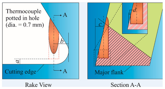
Figure 4.
Thermocouple location.
The dimensions a, b, c, and d are critical for the precise positioning of the thermocouple within the insert, ensuring accurate temperature measurement and maintaining tool integrity. ‘a’ represents the horizontal distance from the cutting edge along the rake face, which is essential for maintaining sensitivity and safety. In this study, ‘a’ varies from 0.15 mm to 0.45 mm, allowing adjustments to optimize thermocouple placement. ‘b’ represents the hole depth that is perpendicular to the rake face, which influences both stability and response, and it is fixed at 1.25 mm across all cases. ‘c’ represents the distance from the center of the hole to the principal flank face, ranging from 0.47 mm to 0.53 mm, facilitating positioning adjustments without compromising tool integrity. ‘d’ represents the minimum residual material thickness of 0.15 mm, ensuring structural integrity and precise temperature measurement.
2.4. ANN Modeling
Artificial neural networks (ANNs) effectively model complex non-linear relationships in manufacturing processes, making them valuable for accurate predictive analysis. In machining and manufacturing processes, the issues associated with artificial neural networks (ANNs) in predictive modeling include data dependency, overfitting, and substantial computing costs. The performance of artificial neural networks is dependent upon the quality of training data; inadequate or noisy input can negatively impact predictive accuracy. Overfitting is a major challenge in an ANN, especially when the model has too many layers or neurons relative to the training data. This results in poor generalization, where the model memorizes training patterns instead of identifying underlying trends. Artificial neural networks (ANNs), on the other hand, involve complex network structures with multiple layers and neurons. The training process, which includes backpropagation and weight adjustments, significantly increases computational demands. The structured methodology was implemented to model artificial neural networks (ANNs) through the use of MATLAB’s NNTOOL (R2024b). The procedure involves the precise steps of data preparation, designing the network architecture, training, validating, and evaluating performance.
2.4.1. Data Acquisition
Experimental data for ANN modeling were obtained through controlled hard turning experiments. The input process parameters were cutting speed (m/min), feed rate (mm/rev), and depth of cut. The cutting temperature and surface roughness were recorded using thermocouples and a surface roughness measuring machine, respectively, for the observed responses. Multiple measurements were obtained for each experiment to ensure reliability, and the average values were incorporated into the modeling process.
2.4.2. Data Pre-Processing
Normalization and Data Partitioning: Neural networks work best when input data are scaled within a uniform range. Thus, all input and output values were normalized between 0 and 1 using min-max scaling. This transformation improves training efficiency and prevents certain features from dominating others due to differing numerical scales. Out of 27 data points, 23 were used for training the artificial neural network model, while the remaining 4 were used for testing its predictive accuracy and generalization capability.
2.4.3. ANN Architecture Design
A Feedforward Backpropagation Neural Network (FFBPNN) was chosen for its capability to approximate non-linear relationships. The designed architecture consisted of the following:
- Input Layer: The input layer comprised 3 neurons, which corresponded to cutting speed, feed rate, and depth of cut.
- Hidden Layer: The optimal number of neurons was determined through trial and error, evaluating configurations with 2, 4, 5, 10, 15, and 20 neurons. A hyperbolic tangent sigmoid activation function (tansig) was used.
- Output Layer: A single neuron in the output layer represented the response, employing a purelin linear activation function for precise output estimation.
2.4.4. Network Training
MATLAB’s NNTOOL was employed to train the ANN model. The following configurations were used:
- Training Algorithm: Levenberg–Marquardt (trainlm) due to its fast convergence properties.
- Training function: Tansig, transfer function was applied to incorporate non-linearity, enabling the network to capture intricate patterns effectively.
- Learning function: Learngdm, learning function was used to refine weight adjustments, promoting faster convergence and minimizing fluctuations during training.
- Performance Function: Mean Squared Error (MSE) function was utilized to evaluate model accuracy by calculating the average squared deviation between predicted and actual outcomes.
- Learning Rate: Initially set between 0.01 and 0.1 and fine-tuned based on validation results.
- Epochs: Maximum of 1000 epochs, with early stopping applied if validation error increased for consecutive iterations.
2.4.5. Model Validation and Performance Evaluation
The ANN model’s accuracy was assessed through regression analysis, showing a strong correlation between predicted outputs and actual results, indicating effective training and reliable predictive capability. The model’s performance was evaluated using the root mean square error (RMSE), which measures the average deviation between predicted and actual values. The final trained model was deployed using MATLAB scripts for predictive analysis and optimization of machining conditions. Table 2 displays the cutting parameters and their respective levels, and Table 3 presents the experimental outcomes.
Table 2.
Cutting parameters and their levels for MCFA turning of AISI 52100 alloy steel.
Table 3.
Experimental result in MCFA turning of AISI 52100 alloy steel.
3. Results and Discussion
Design-Expert software (Version 13) was employed for statistical evaluation, analysis of cutting parameter interactions, regression modeling, and the creation of diagnostic and contour plots, whereas MATLAB was utilized for predictive modeling using an ANN.
3.1. Effect of Cutting Parameters on Cutting Temperature
Figure 5a depicts the effect of cutting speed and feed rate on cutting temperature. The cutting speed ranged from 80 m/min to 140 m/min, while the feed rate varied between 0.08 mm/rev and 0.14 mm/rev. A noticeable increase in temperature was observed with higher cutting speeds. At 80 m/min, the temperature remained around 520 °C, whereas at 140 m/min, it exceeded 660 °C, primarily due to increased friction and plastic deformation. The feed rate had a comparatively lower influence, but an increase from 0.08 mm/rev to 0.14 mm/rev at 120 m/min raised the temperature by nearly 60 °C. The highest thermal intensity was recorded at 140 m/min cutting speed and 0.14 mm/rev feed rate, while the lowest temperatures occurred at 80 m/min and 0.08 mm/rev, indicating minimal thermal effects. Figure 5b shows that as the cutting speed increased from 80 m/min to 140 m/min, the temperature rose from 520 °C to over 660 °C due to higher friction and plastic deformation at the tool-chip interface. Similarly, an increase in the depth of cut from 0.15 mm to 0.45 mm led to a further rise in temperature, exceeding 660 °C, as greater material removal required higher energy input. The elevated temperatures adversely affected the surface integrity of the machined component; thus, the study underscored the necessity of optimizing machining parameters to minimize thermal effects.
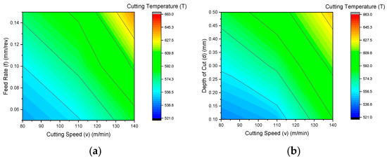
Figure 5.
Contour Plot of cutting temperature for the following: (a) cutting speed vs. feed rate; (b) cutting speed vs. depth of cut.
3.2. Effect of Cutting Parameters on Surface Roughness
Figure 6a depicts the effect of cutting speed (v) and feed rate (f) on surface roughness. At a cutting speed of 80 m/min and a feed rate of 0.14 mm/rev, surface roughness exceeded 0.072 µm, indicating a rougher finish. However, as the cutting speed increased to 140 m/min while maintaining a lower feed rate of approximately 0.06 mm/rev, roughness significantly reduced to around 0.016 µm, demonstrating an improved surface finish. The findings revealed that higher cutting speeds with lower feed rates resulted in superior surface quality, whereas elevated feed rates negatively impacted the finish due to increased material deformation and intensified tool–workpiece interaction. Figure 6b depicts the influence of cutting speed (v) and depth of cut (d) on surface roughness. At a lower cutting speed of 80 m/min with a greater depth of cut around 0.50 mm, roughness exceeded 0.072 µm, signifying surface deterioration. As the cutting speed rose above 120 m/min with a shallower depth of cut near 0.15 mm, roughness significantly declined, reaching approximately 0.016 µm. This trend confirmed that a combination of higher cutting speeds and lower depths of cut promoted better surface integrity, whereas deeper cuts at low speeds intensified surface irregularities due to increased tool engagement and material deformation effects.
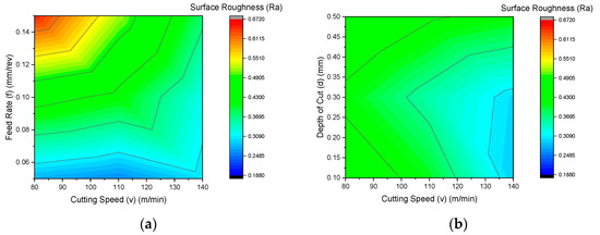
Figure 6.
Contour plot of surface roughness for the following: (a) cutting speed vs. feed rate; (b) cutting speed vs. depth of cut.
3.3. Cutting Temperature Prediction by RSM
The quadratic model is suggested by response surface methodology. Table 4 exhibits the selection of an appropriate model for cutting temperature, and the highest order polynomial model was selected, ensuring that the additional terms are statistically significant and the model remains free from aliasing. The analysis of the sequential model sum of squares showed that the quadratic model, compared to the 2FI model, has the highest F-value of 57.09 and p-value of <0.0001. “Lack of Fit F-value” of 3.75 indicated that the “Lack of Fit” is statistically insignificant when compared to the pure error. There was an 8.64% chance that a “Lack of Fit F-value” of this magnitude may be attributed to random variations. “Lack of Fit” was not significant and the model provided a good fit to the data.
Table 4.
Selection of adequate model for cutting temperature.
3.3.1. Quadratic Regression Model for Cutting Temperature
The correlation between cutting temperature and machining parameters was established using regression analysis. The response function representing cutting temperature is expressed as where denotes cutting speed in m/min, is the feed rate in mm/rev, and is the depth of cut in mm. A second-order polynomial relationship was selected, which was formulated into equations using both coded and actual variables. The equations in coded factors and their corresponding actual factor versions can be used to predict cutting temperature for specific parameter levels.
The mathematical expression for cutting temperature in coded factors (Equation (1)):
The mathematical expression for cutting temperature in actual factors (Equation (2)):
The coefficients of the quadratic regression model were determined using Design-Expert software, which employs least squares regression for precise coefficient estimation. The calculated values of coded coefficients for a quadratic model of cutting temperature are shown in Table 5.
Table 5.
Coded coefficients for quadratic model of cutting temperature.
The coefficient estimates showed the relative importance of the parameters. Accordingly, cutting speed, depth of cut, and quadratic term of cutting speed () with coefficients of 27.05, 20.18, and 20.79 were more influential on cutting temperature. The coefficient associated with the cutting speed, feed rate, and depth of cut were positive, indicating that the cutting temperature increases with increasing the cutting parameters. The coefficients of the parameters associated with the interaction of cutting speed, feed rate, and depth of cut were positive. Therefore, an increase in these variables increases the cutting temperature except for the quadratic term of the depth of cut since the associated coefficient is negative. The Variance Inflation Factor (VIF) for each term in the model was around 1 and indicated the absence of multicollinearity.
3.3.2. Diagnostic Plots for Cutting Temperature
The normal probability plot of residuals, predicted vs. actual values, residuals versus predicted values, and residuals versus run number were used to check the adequacy of the proposed model. Figure 7a illustrates the normal probability plot of residuals for cutting temperature, demonstrating that the residuals predominantly align with the reference line, indicating a normal distribution of errors. Figure 7b presents a comparison between predicted and actual values, showing a close alignment, which confirms the model’s predictive accuracy. Figure 7c depicts the residuals plotted against predicted values, with all residuals falling within the range of −4.1479 to 4.1479, suggesting no obvious patterns and validating the model’s suitability. Figure 7d displays residuals versus run numbers, with residuals randomly fluctuating around the zero line, implying that the errors are independent and supporting the assumption of a valid linear relationship.
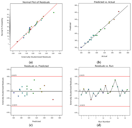
Figure 7.
Diagnostic Plots for cutting temperature for the following: (a) residuals vs. normal probability; (b) predicted vs. actual values; (c) residuals vs. predicted values; (d) residuals vs. run numbers for cutting temperature.
3.4. Surface Roughness Prediction by RSM
The sequential model sum of squares test evaluates the highest-order polynomial with non-aliased terms. Typically, models with lower p-values and higher F-values are preferred for implementation. Table 6 outlines the selection of the most suitable model for surface roughness. Based on the analysis, the quadratic versus 2FI model was recommended due to its superior performance, characterized by an F-value of 49.85 and a p-value of less than 0.0001. The Lack of Fit F-value of 3.29 suggested that the lack of fit was not significant compared to pure error, with only a 10.86% probability of such a value arising due to noise. Consequently, the lack of fit was deemed insignificant, confirming the model’s adequacy for predictive accuracy.
Table 6.
Optimal model selection for surface roughness prediction.
3.4.1. Quadratic Regression Model for Surface Roughness
The relationship between surface roughness and cutting parameters was developed using regression methods. The regression equations established a correlation between the significant terms obtained from Analysis of Variance (ANOVA) analysis, namely cutting speed, feed rate, depth of cut, and their interactions. The competency of the model was tested using correlation coefficients, and acceptance was based on high to very high coefficients of correlation. Developed models can be employed to predict values of surface roughness from any combination within the range of variables studied. The equations below are in terms of coded factors and actual factors.
The mathematical expression for surface roughness in coded factors (Equation (3)):
The mathematical expression for surface roughness in coded factors (Equation (4)):
Table 7 presents the coded coefficients for the quadratic model of surface roughness. These coefficients provide an estimate of the practical impact each term has on the response variable. Among the factors evaluated, cutting speed, feed rate, and the quadratic term of feed rate, with coefficients of 0.0677, 0.0449, and −0.0515, respectively, were identified as having the greatest impact on surface roughness. However, it is crucial to understand that the coefficient’s magnitude by itself does not confirm statistical significance, as the determination of significance also takes into account the variability in the response data.
Table 7.
Coded coefficients for quadratic model of surface roughness.
3.4.2. Diagnostic Plots for Surface Roughness
Figure 8a presents the normal probability plot of residuals for surface roughness, indicating that the residuals align closely with the reference line, confirming a normal distribution of errors. Figure 8b depicts the predicted versus actual values of surface roughness (), demonstrating a strong correlation and suggesting a high degree of model accuracy. Figure 8c illustrates the residuals against the predicted values, showing no discernible pattern, with residuals evenly distributed on both positive and negative sides. This implies that the model is appropriate, and the assumption of constant variance holds true. Figure 8d displays residuals plotted against run numbers, revealing the absence of heteroscedasticity and non-linearity, further validating the regression model’s reliability.
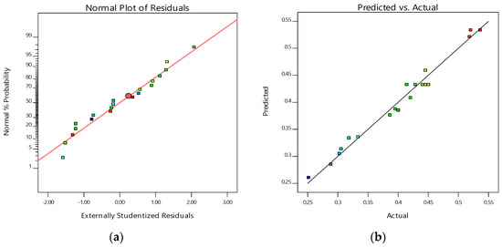
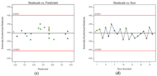
Figure 8.
Validation plots for surface roughness for the following: (a) residuals vs. normal probability; (b) predicted vs. actual values; (c) residuals vs. predicted values; (d) residuals vs. run numbers for cutting temperature.
3.5. Cutting Temperature Prediction by ANN
MATLAB’s NNTOOL was used for ANN modeling, leveraging its powerful neural network toolbox for training and validation. An ANN model was developed using a routine that uses a feedforward backpropagation algorithm. Out of the 27 readings, 23 were selected for training the model, and 4 readings were used to test the model (Table 2). Networks of different architectures were trained at different cycles. Gradual changes were made to the hidden layer and neurons. As a quadratic scoring rule, the RMSE was used to quantify the magnitude of the average error. RMSE is particularly beneficial when the objective is to minimize significant errors. The ANN model was trained in different configurations. The RMSE values and the coefficients of determination were calculated. The architecture of the neural network is composed of three neurons in the input layer, two neurons in the hidden layer, and one neuron in the output layer. This architecture, with a configuration of 3-2-1, achieved the lowest MSE value of 0.005233 after 1000 cycles. The calculated coefficient of determination for this setup was determined to be 0.98. Several other networks with lower RMS error values were rejected due to poor training and validation results. The combination of some networks during training was able to achieve 100% efficiency, but these networks were rejected because of the higher RMS error. Priority was given to the network, which always results in very low RMS error values and having validation and training data values greater than 95%. To avoid overfitting and achieve optimal model generalization while preserving accuracy, the study used early stopping strategies during the ANN training. Table 8 displays the training parameters used as input for the ANN training of cutting temperature.
Table 8.
ANN training parameters for cutting temperature.
Figure 9 shows the architecture 3-2-1 of the ANN model for cutting temperature.
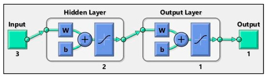
Figure 9.
Architecture 3-2-1 of the ANN model for cutting temperature.
Figure 10 illustrates the RMSE values for different ANN configurations used to predict cutting temperature. The x-axis represented RMSE values, while the y-axis listed various network architectures. Each bar depicted the RMSE of a specific ANN model, where a lower value indicated better prediction accuracy. The variation in RMSE showed the impact of network structure on performance, with some configurations demonstrating superior learning capabilities. A specific RMSE value of 0.005233 was highlighted, suggesting an optimal architecture with minimal error. The highest RMSE, 0.32571, indicated a less effective model, possibly due to under fitting or overfitting. The results emphasized the importance of selecting an appropriate ANN structure to achieve accurate predictions while maintaining a balance between model complexity and generalization.
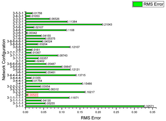
Figure 10.
Root mean squared error graph for ANN training data on cutting temperature.
Figure 11 presents the efficiency of regression for different ANN configurations during the training phase for cutting temperature prediction. Each bar depicted the efficiency of a specific ANN model, where higher values indicated better predictive performance. The variation in efficiency showed the influence of network structure on model accuracy, with some architectures achieving superior regression efficiency. A specific efficiency value of 0.99041 was highlighted, suggesting an optimal configuration. The results emphasized the importance of selecting a well-structured ANN model to achieve high regression efficiency and reliable predictions.
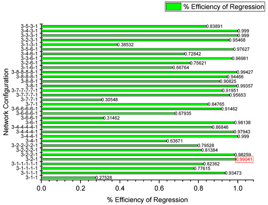
Figure 11.
Efficiency of regression graph for ANN training data on cutting temperature.
Figure 12 illustrates the regression efficiency of different ANN configurations during the validation phase for cutting temperature prediction. The x-axis represented the percentage efficiency of validation, while the y-axis displayed various network architectures. The variation in efficiency reflected the influence of network structure on model generalization. A specific efficiency value of 0.99691 was highlighted, suggesting an optimal configuration. The results emphasized the importance of selecting a well-structured ANN model to achieve high validation efficiency and reliable predictions. Further testing on unseen data was necessary to confirm model robustness before deployment.
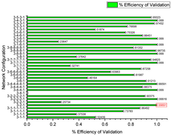
Figure 12.
Regression efficiency graph for validation of cutting temperature.
Figure 13 presents the validation performance of the 3-2-1 neural network architecture for cutting temperature. The x-axis represents the number of training cycles (epochs), while the y-axis denotes the mean squared error (MSE). The graph consists of three curves corresponding to the training, validation, and testing phases. Initially, the MSE decreases sharply, indicating effective learning. The network achieves its optimal validation performance at 45 epochs, with a minimum MSE of 0.00523, after which the error stabilizes. This confirms the model’s reliability in accurately predicting cutting temperature while maintaining generalization across validation and test datasets.
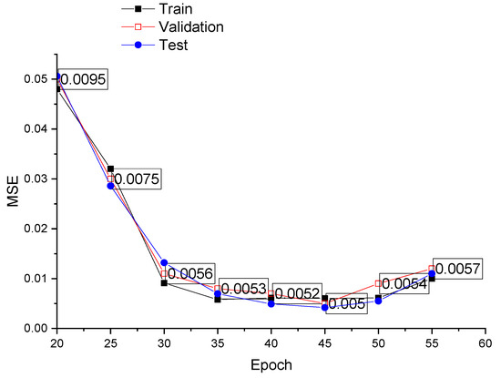
Figure 13.
Validation performance of the 3-2-1 architecture for cutting temperature.
Figure 14 shows the regression plot of training, validation, and test performances for cutting temperature. The fit for all datasets was excellent, with R-values of 0.99 in each case. The correlation coefficient corresponding to all the parameters is displayed, which clearly indicates the perfect fit since all the accumulated data are found near the line.
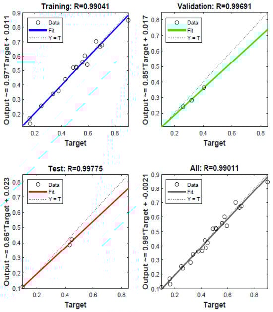
Figure 14.
Plot of training, validation, and test performances for cutting temperature.
The analysis of the error rate to predict the response was performed by simulating the selected network using the four test values selected in the 27 run experiments. Table 9 shows the experimental values of cutting temperature obtained at the experimental stage, along with the values and error rates predicted by the ANN network.
Table 9.
Cutting temperature prediction by ANN.
3.6. Surface Roughness Prediction by ANN
The architecture of the neural network comprised three neurons in the input layer, twenty neurons in the hidden layer, and one neuron in the output layer. This architecture, with a configuration of 3-20-1, achieved the lowest MSE value of 0.0056035 after 1000 cycles. The calculated coefficient of determination yielded a value of 0.97. Table 10 presents the ANN input training parameters for surface roughness, and Figure 15 shows the architecture 3-20-1 of the ANN model for surface roughness.
Table 10.
ANN training parameters for surface roughness.
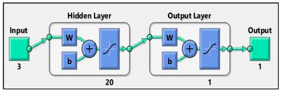
Figure 15.
Architecture 3-20-1 of the ANN model for surface roughness.
Figure 16 displays the RMSE values for different ANN configurations used to predict surface roughness. RMS error analysis was performed for 20 network configurations. The x-axis in the figure represents various network architectures, while the y-axis displays the corresponding RMS error values. Among the tested models, the 3-20-1 network demonstrated the lowest RMS error of 0.0009105, reflecting higher accuracy. Although a few other configurations also exhibited low RMS values, they were disregarded due to inadequate performance in training and validation. These results highlighted the necessity of choosing an ANN model that maintains an optimal balance between error reduction and overall performance. Early stopping was applied to prevent overfitting by halting training when validation error increased, ensuring optimal generalization and accuracy.
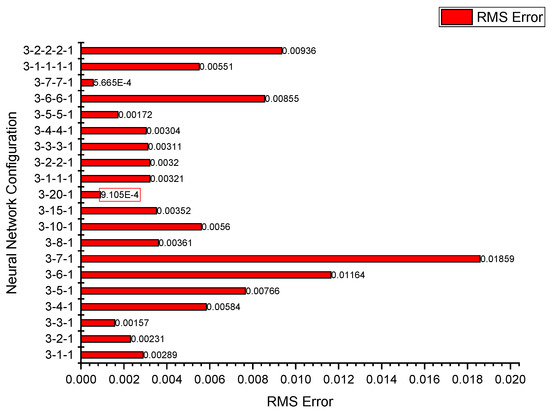
Figure 16.
Root mean squared error graph for ANN training data on surface roughness.
Figure 17 presents the efficiency of the regression graph for the ANN training data on surface roughness. The training dataset was utilized to develop the ANN model by minimizing errors and establishing a mathematical correlation between inputs and outputs. The training efficiency should exceed 95% for optimal performance. The 3-20-1 network achieved 99.27% efficiency, as depicted in the figure. Although certain network architectures exhibited marginally higher training efficiency, they were excluded due to their suboptimal root mean squared (RMS) error values. This selection approach ensures a balance between regression accuracy and error minimization, leading to a well-trained ANN model suitable for predictive analysis.
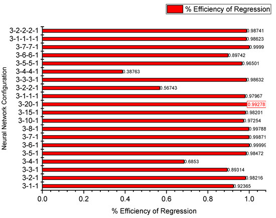
Figure 17.
Efficiency of regression graph for ANN training data on surface roughness.
Figure 18 shows a regression efficiency graph for validation of cutting temperature. The validation phase assesses the neural network’s performance on novel data after the training phase, ensuring its predictive capability. This process verifies the input-output relationships established during training by testing the model on randomly selected data points. The validation efficiency should exceed 95% for reliable model performance. The 3-20-1 network configuration achieved 99.11% validation efficiency, as shown in the figure, indicating strong generalization. While some configurations demonstrated comparable efficiency, they were rejected due to higher RMS error values. The validation process confirms the model’s accuracy and robustness, which is crucial for ensuring reliable predictions in machining applications.
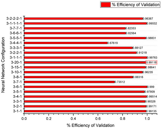
Figure 18.
Regression efficiency graph for validation of surface roughness.
Figure 19 illustrates the validation performance of the 3-20-1 neural network architecture for cutting temperature. The x-axis represents the number of epochs, indicating the training cycles, while the y-axis denotes the mean squared error (MSE). The graph presents three plots corresponding to the training, validation, and testing phases. Initially, the MSE is high but rapidly declines within the first few epochs, signifying effective learning. The model stabilizes thereafter, achieving its best performance at a minimal MSE and ensuring reliable predictive capability. The best performance is observed at an MSE of approximately 0.0009105 at around 16 epochs. The validation curve closely follows the training curve, confirming minimal overfitting and robust generalization of the model.
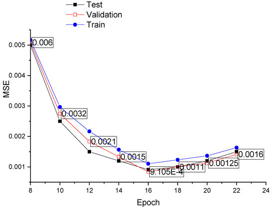
Figure 19.
Validation performance of the 3-20-1 architecture for surface roughness.
Figure 20 shows the regression plot of training, validation, and test performances for surface roughness. The regression plots illustrated the correlation between the network’s outputs and the targets. The training data showed a strong correlation, with R-values exceeding 0.97 in both the validation and test results.
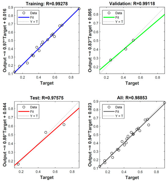
Figure 20.
Plot of training, validation, and test performances for surface roughness.
Table 11 above shows the experimental values of surface roughness obtained at the experimental stage along with the values and error rates predicted by the ANN network.
Table 11.
Prediction of surface roughness by ANN.
Table 12 and Table 13 compare experimental results with those from the QR and ANN models, showing the percentage error for cutting temperature and surface roughness, respectively. The QR and ANN models both demonstrated a good correlation with experimental values, but the ANN model closely matched the experimental results. The ANN model provided the most accurate predictions with minimum average error percentages of 1.95% for cutting temperature and 1.42% for surface roughness, whereas the QR model showed higher errors of 4.73% for cutting temperature and 5.79% for surface roughness (). Therefore, the ANN model is recommended for precise prediction of cutting temperature and surface roughness during hard turning of AISI 52100 steel within the experimental range. The ANN’s predictive capability was found superior to that of the RSM.
Table 12.
Comparison of experimental, QR, and ANN results and % of error for cutting temperature.
Table 13.
Comparison of experimental, QR and ANN results and % of error for surface roughness.
4. Comparative Study
An experimental study was carried out to examine the effects of dry, MQL, and MCFA-assisted hard turning on cutting temperature and surface roughness under identical cutting conditions. The main objective was to assess the MCFA’s effectiveness in lowering the cutting temperature and enhancing the surface finish, which, in turn, improved the machining performance, while minimizing environmental impact. Table 14 presents the Ra values recorded under dry, MQL, and MCFA conditions. The results showed a considerable improvement in surface roughness with the MCFA, indicating a reduction of 18.59% to 46.18% compared to dry-hard turning and 10.24% to 24.14% relative to MQL-assisted machining. The observed improvement in surface roughness with the MCFA suggests a positive influence on surface integrity, which may contribute to enhanced fatigue life, wear resistance, and functional performance of machined components.
Table 14.
Arithmetic average surface roughness (Ra) under dry, MQL, and MCFA environments.
Table 15 depicts the cutting temperatures recorded under the same machining conditions for the different cutting environments: dry, MQL, and the MCFA. The findings revealed a notable decrease in cutting temperature with the MCFA, indicating a reduction of 9.21% to 16.96% compared to dry machining and a 4.60% to 9.19% reduction relative to MQL-assisted turning. This reduction underscores the enhanced cooling and lubrication efficiency of the MCFA, which significantly reduces heat generation and enhances heat dissipation at the cutting zone and its subsequent impact on machining performance. The significant reduction in cutting temperature and improvement in surface finish validate the MCFA as an effective and eco-friendly substitute for traditional cooling techniques, positioning it as a practical option for enhancing the machining performance.
Table 15.
Cutting temperature under dry, MQL, and MCFA environments.
5. Conclusions
The ANN model, which employs a multilayer feedforward network, demonstrated the lowest average error rate in accurately predicting the response when compared to the QR model. The ANN model demonstrated mean errors of 1.95% and 1.42% in relation to the cutting temperature and surface roughness (), respectively. In contrast, the QR model exhibited mean errors of 4.73% for cutting temperature and 5.79% for surface roughness. The ANN model demonstrated superior prediction accuracy compared to the RSM in both the surface roughness and cutting temperature due to its ability to capture non-linear interactions. The findings suggested that the ANN is a more robust tool for process optimization in hard turning under MCFA conditions. However, it is important to note that the ANN model was trained on a small dataset, and its performance could potentially be enhanced with a more extensive experimental framework, which includes a wider range of process conditions. Additionally, the study found that the MCFA significantly improved surface roughness and decreased cutting temperature, making it an eco-friendly alternative to traditional cooling techniques compared to dry and MQL-assisted hard turning, thus contributing to sustainable manufacturing practices. An ANN model enabled the precise forecasting of cutting temperature and surface roughness during the MCFA turning of AISI 52100 alloy steel within the experimental domain.
Future research should enhance the accuracy of the artificial neural network (ANN) model by incorporating hybrid optimization techniques, expanding the dataset with a wider range of cutting parameters, integrating real-time sensor-based data with ANN, and exploring deep learning approaches.
Author Contributions
Conceptualization, S.M. and R.B.P.; methodology, S.M.; software, S.M.; validation, S.M., R.B.P., and S.A.-D.; formal analysis, S.M.; investigation, S.M.; resources, S.M. and R.B.P.; data curation, S.M.; writing—original draft preparation, S.M. and R.B.P.; writing—review and editing, S.M., R.B.P., and S.A.-D.; visualization, S.M., R.B.P., and S.A.-D.; supervision, S.M. and R.B.P.; project administration, R.B.P. All authors have read and agreed to the published version of the manuscript.
Funding
This research received no external funding.
Data Availability Statement
Dataset available on request from the authors.
Conflicts of Interest
The authors declare no conflicts of interest.
Abbreviations and Symbols
The following abbreviations and symbols are used in this manuscript:
| AISI | American Iron and Steel Institute |
| OHNS | Oil-Hardened Non-Shrinking |
| AI | Artificial Intelligence |
| ANNs | artificial neural networks |
| ANFIS | Adaptive Neuro-Fuzzy Inference Systems |
| ANOVA | Analysis of Variance |
| CBN | Cubic Boron Nitride tool |
| CC | Coated Ceramic |
| EDM | Electric Discharge Machining |
| GP | genetic programming |
| HRC | Hardness Rockwell C (scale for hardness) |
| HST | High-Speed Turning |
| LM | Levenberg–Marquardt |
| MAPE | Mean Absolute Percentage Error |
| MRA | Multivariable Regression Analysis |
| MCFA | minimal cutting fluid application |
| MQL | minimum quantity lubrication |
| QR | quadratic regression |
| R | Correlation Coefficient Factor |
| R2 | coefficient of determination |
| RMSE | root mean square error |
| RSM | response surface methodology |
| VIF | Variance Inflation Factor |
| Seq SS | Sequential Sum of Squares |
| Adj MS | Adjusted Mean Square |
| F-Value | F-Ratio (test statistic used to determine significance in ANOVA) |
| cutting speed (m/min) | |
| feed rate (mm/rev) | |
| depth of cut (mm) | |
| Arithmetic Average Roughness | |
| Maximum peak-to-valley height | |
| Average peak-to-valley height |
References
- Astakhov, V.P. Machining of Hard Materials—Definitions and Industrial Applications. In Machining of Hard Materials; Springer: Berlin/Heidelberg, Germany, 2011. [Google Scholar]
- Anand, A.; Behera, A.K.; Das, S.R. An Overview on Economic Machining of Hardened Steels by Hard Turning and Its Process Variables. Manuf. Rev. 2019, 6, 4. [Google Scholar] [CrossRef]
- Özel, T.; Karpat, Y. Prediction of Surface Roughness and Tool Wear in Finish Dry Hard Turning Using Back Propagation Neural Networks. In Proceedings of the 17th International Conference on Production Research, Blacksburg, VA, USA, 3–7 August 2003. [Google Scholar]
- Nalbant, M.; Gokkaya, H.; Toktaş, I. Comparison of Regression and Artificial Neural Network Models for Surface Roughness Prediction with the Cutting Parameters in CNC Turning. Model. Simul. Eng. 2007, 2007, 092717. [Google Scholar] [CrossRef]
- Quiza, R.; Figueira, L.; Davim, J.P. Comparing Statistical Models and Artificial Neural Networks on Predicting the Tool Wear in Hard Machining D2 AISI Steel. Int. J. Adv. Manuf. Technol. 2008, 37, 641–648. [Google Scholar] [CrossRef]
- Leo Dev Wins, K.; Varadarajan, A.S. Simulation of Surface Milling of Hardened AISI4340 Steel with Minimal Fluid Application Using Artificial Neural Network. Adv. Prod. Eng. Manag. 2012, 7, 51. [Google Scholar] [CrossRef]
- Chandrasekaran, M.; Muralidhar, M.; Krishna, C.M.; Dixit, U.S. Application of Soft Computing Techniques in Machining Performance Prediction and Optimization: A Literature Review. Int. J. Adv. Manuf. Technol. 2010, 46, 445–464. [Google Scholar] [CrossRef]
- Sethi, D.; Kumar, V. Modeling of Tool Wear in Turning En 31 Alloy Steel Using Coated Carbide Inserts. Int. J. Manuf. Mater. Mech. Eng. 2012, 2, 34–51. [Google Scholar] [CrossRef][Green Version]
- Aouici, H.; Yallese, M.A.; Chaoui, K.; Mabrouki, T.; Rigal, J.F. Analysis of Surface Roughness and Cutting Force Components in Hard Turning with CBN Tool: Prediction Model and Cutting Conditions Optimization. Measurement 2012, 45, 344–353. [Google Scholar] [CrossRef]
- Bouacha, K.; Yallese, M.A.; Mabrouki, T.; Rigal, J.F. Statistical Analysis of Surface Roughness and Cutting Forces Using Response Surface Methodology in Hard Turning of AISI 52100 Bearing Steel with CBN Tool. Int. J. Refract. Met. Hard Mater. 2010, 28, 349–361. [Google Scholar] [CrossRef]
- Attanasio, A.; Ceretti, E.; Giardini, C.; Cappellini, C. Tool Wear in Cutting Operations: Experimental Analysis and Analytical Models. J. Manuf. Sci. Eng. 2013, 135, 051012. [Google Scholar] [CrossRef]
- Chinchanikar, S.; Choudhury, S.K. Machining of Hardened Steel—Experimental Investigations, Performance Modeling and Cooling Techniques: A Review. Int. J. Mach. Tools Manuf. 2015, 89, 95–109. [Google Scholar] [CrossRef]
- Cica, D.; Sredanovic, B.; Kramar, D. Modelling of Tool Life and Surface Roughness in Hard Turning Using Soft Computing Techniques: A Comparative Study. Int. J. Mater. Prod. Technol. 2015, 50, 49–64. [Google Scholar] [CrossRef]
- Mia, M.; Dhar, N.R. Response Surface and Neural Network Based Predictive Models of Cutting Temperature in Hard Turning. J. Adv. Res. 2016, 7, 1035–1044. [Google Scholar] [CrossRef] [PubMed]
- Panda, A.; Sahoo, A.K.; Panigrahi, I.; Rout, A.K. Investigating Machinability in Hard Turning of AISI 52100 Bearing Steel through Performance Measurement: QR, ANN and GRA Study. Int. J. Automot. Mech. Eng. 2018, 15, 4935–4961. [Google Scholar] [CrossRef]
- Labidi, A.; Tebassi, H.; Belhadi, S.; Khettabi, R.; Yallese, M.A. Cutting Conditions Modeling and Optimization in Hard Turning Using RSM, ANN and Desirability Function. J. Fail. Anal. Prev. 2018, 18, 1017–1033. [Google Scholar] [CrossRef]
- Zerti, A.; Yallese, M.A.; Zerti, O.; Nouioua, M.; Khettabi, R. Prediction of Machining Performance Using RSM and ANN Models in Hard Turning of Martensitic Stainless Steel AISI 420. Proc. Inst. Mech. Eng. C J. Mech. Eng. Sci. 2019, 233, 4439–4462. [Google Scholar] [CrossRef]
- Kumar, R.; Sahoo, A.K.; Das, R.K.; Panda, A.; Mishra, P.C. Modelling of Flank Wear, Surface Roughness and Cutting Temperature in Sustainable Hard Turning of AISI D2 Steel. Procedia Manuf. 2018, 20, 406–413. [Google Scholar] [CrossRef]
- Elsadek, A.A.; Gaafer, A.M.; Mohamed, S.S.; Mohamed, A.A. Prediction and Optimization of Cutting Temperature on Hard-Turning of AISI H13 Hot Work Steel. SN Appl. Sci. 2020, 2, 540. [Google Scholar] [CrossRef]
- Adizue, U.L.; Tura, A.D.; Isaya, E.O.; Farkas, B.Z.; Takács, M. Surface Quality Prediction by Machine Learning Methods and Process Parameter Optimization in Ultra-Precision Machining of AISI D2 Using CBN Tool. Int. J. Adv. Manuf. Technol. 2023, 129, 1375–1394. [Google Scholar] [CrossRef]
- Şahin, Y. Prediction of Surface Roughness When Maching Mild Steel Using Statistical Methods. Adv. Mater. Process. Technol. 2024, 10, 1593–1609. [Google Scholar] [CrossRef]
- Bañon, F.; Martin, S.; Vazquez-Martinez, J.M.; Salguero, J.; Trujillo, F.J. Predictive Models Based on RSM and ANN for Roughness and Wettability Achieved by Laser Texturing of S275 Carbon Steel Alloy. Opt. Laser Technol. 2024, 168, 109963. [Google Scholar] [CrossRef]
- Mebrek, H.; Mansouri, S.; Touggui, Y.; Ameddah, H.; Yallese, M.A.; Benia, H.M. Predictive modeling and optimization of cutting parameters in high speed hardened turning of aisi D2 steel using rsm, ann and desirability function. Surf. Rev. Lett. 2024, 31, 2450036. [Google Scholar] [CrossRef]
- Bien, D.X. Predictive Modeling of Surface Roughness in Hard Turning with Rotary Cutting Tool Based on Multiple Regression Analysis, Artificial Neural Network, and Genetic Programing Methods. Proc. Inst. Mech. Eng. B J. Eng. Manuf. 2024, 238, 137–150. [Google Scholar] [CrossRef]
- Hossain, S.; Abedin, M.Z.; Saha, R.K.; Touhiduzzaman, M.; Hossen, M.J. Optimization of Cutting Temperature and Surface Roughness in CNC Turning of Ti-6Al-4V Alloy Using Response Surface Methodology. Heliyon 2025, 11, e41051. [Google Scholar] [CrossRef] [PubMed]
- Vasconcelos, G.A.V.B.; Francisco, M.B.; da Costa, L.R.A.; Ribeiro Junior, R.F.; Melo, M.d.L.N.M. Prediction of Surface Roughness in Duplex Stainless Steel Face Milling Using Artificial Neural Network. Int. J. Adv. Manuf. Technol. 2024, 133, 2031–2048. [Google Scholar] [CrossRef]
- Ambhore, N.; Gaikwad, M.; Patil, A.; Sharma, Y.; Manikjade, A. Predictive Modeling and Optimization of Dry Turning of Hardened Steel. Int. J. Interact. Des. Manuf. 2023, 18, 6281–6287. [Google Scholar] [CrossRef]
- Kumar, R.; Rafighi, M.; Özdemir, M.; Şahinoğlu, A.; Kulshreshta, A.; Singh, J.; Singh, S.; Prakash, C.; Bhowmik, A. Modeling and Optimization of Hard Turning: Predictive Analysis of Surface Roughness and Cutting Forces in AISI 52100 Steel Using Machine Learning. Int. J. Interact. Des. Manuf. (IJIDeM) 2024. [Google Scholar] [CrossRef]
- Sukonna, R.T.; Zaman, P.B.; Dhar, N.R. Estimation of Machining Responses in Hard Turning under Dry and HPC Conditions Using Different AI Based and Statistical Techniques. Int. J. Interact. Des. Manuf. 2022, 16, 1705–1725. [Google Scholar] [CrossRef]
- Hoyne, A.C.; Nath, C.; Kapoor, S.G. On Cutting Temperature Measurement during Titanium Machining with an Atomization-Based Cutting Fluid Spray System. J. Manuf. Sci. Eng. Trans. ASME 2015, 137, 024502. [Google Scholar] [CrossRef]
Disclaimer/Publisher’s Note: The statements, opinions and data contained in all publications are solely those of the individual author(s) and contributor(s) and not of MDPI and/or the editor(s). MDPI and/or the editor(s) disclaim responsibility for any injury to people or property resulting from any ideas, methods, instructions or products referred to in the content. |
© 2025 by the authors. Licensee MDPI, Basel, Switzerland. This article is an open access article distributed under the terms and conditions of the Creative Commons Attribution (CC BY) license (https://creativecommons.org/licenses/by/4.0/).