Abstract
In modern manufacturing, cutting tools are essential for cutting processes, and their wear state directly affects the processing accuracy, production efficiency, and product quality. Identification of the tool-wear state using a single sensor is insufficient to satisfy the requirements of high-precision, high-efficiency machining. To address this problem, this paper proposes a novel approach to identify the tool-wear state using information fusion technology and the sparrow search algorithm (SSA)–backpropagation (BP) neural network framework. This method uses a principal component analysis (PCA) to fuse multi-domain features extracted from three-way vibration signals, power signals, and temperature signals. Subsequently, the optimal initial threshold and weight of the BP neural network are optimized using the SSA to prevent the network from falling into the local optimum and accelerate the convergence of the algorithm. Lastly, a tool-wear-state identification model based on the SSA–BP neural network is constructed. Experimental results show that the proposed method has an identification accuracy of 98.33%, precision rate of 98.81%, recall rate of 97.96%, and F1 score of 98.36%.
1. Introduction
During CNC machine tool cutting, the tool-wear state directly affects the surface quality, processing efficiency, and processing accuracy of the workpiece [1,2]. Approximately 20% of CNC machine tool failures are attributable to tool wear [3]. Hence, identification of the tool-wear status is the focus of extensive attention from engineers and scholars. Tool-wear identification methods can be divided into direct and indirect approaches [4]. Direct methods require halting CNC machine tool operations to capture images of the worn tool using charge-coupled-device cameras and lighting units. The tool-wear state is then identified from the images. However, this approach reduces the workpiece processing efficiency. In indirect methods, sensors such as vibration, cutting-force, acoustic-emission, and current sensors are installed in the CNC machine tool, and the tool-wear status is analyzed using the signals of various sensors [5,6]. This method can identify the tool-wear status without interrupting the machining process, while reducing the complexity of detection operations. Therefore, at present, tool-wear-state identification is mainly based on indirect methods.
In recent years, numerous scholars have explored indirect methods for identifying tool-wear status. Wang et al. [7] collected vibration signals during workpiece machining and used a support vector machine (SVM) to identify the tool-wear status. Chen et al. [8] performed linear interpolation on vibration signals to improve the data integrity and used the complete vibration signal data to construct a tool-wear-state identification model based on a convolutional neural network. Aldekoa et al. [9] analyzed the correlation between the servo motor variables and the tool status of a broaching machine, and used a regression machine learning algorithm to effectively predict the tool-wear status. Zhang et al. [10] constructed a convolutional neural network model with multi-scale features based on the cutting-force signals extracted during machining, thereby improving the accuracy of tool-wear-state identification. Wang et al. [11] used the clustering energy of acoustic-emission burst signals to evaluate the tool-wear state through a linear fitting method.
Notably, in these methods, the signal information provided by a single sensor indicates only a single physical quantity, which limits enhancement of the accuracy of tool-wear identification. Multi-sensor information fusion technology can fully leverage the complementary advantages of multiple sensor signals, ensure the reliability and comprehensiveness of the monitoring signals, and improve the accuracy of tool-wear-status identification [12,13,14,15]. For tool-wear-state identification, Gomes et al. [16] combined vibration and acoustic-emission signals to identify the most relevant features of tool wear using recursive feature elimination and SVM. Gao et al. [17] collected three-dimensional vibration signals, three-dimensional force signals, and acoustic-emission signals during workpiece processing and performed multi-sensor, mixed-field-feature information fusion. Additionally, deep neural networks were incorporated to identify the tool-wear status. Niaki et al. [18] performed feature fusion on power and vibration signals based on principal component analysis (PCA) to eliminate redundant and irrelevant feature data and designed a neural network with Bayesian regularization to improve the accuracy of tool-wear-state identification. Ni et al. [19] used vibration and acoustic-emission signals for multi-domain feature fusion and proposed a dual-attention model based on information graphs to identify the tool-wear state. Xu et al. [20] developed a wavelet-packet-decomposition method to extract the optimal characteristic frequency bands of acoustic-emission and vibration-acceleration signals, and combined it with a backpropagation (BP) neural network to identify the tool-wear status.
Based on this review, a comprehensive evaluation is performed that considers the cost, installation mode, environmental adaptability, and measurement accuracy. For this study, three-way vibration signals, power signals, and temperature signals are selected as the primary data for tool-wear-state identification. The three-way vibration signal, which is closely related to the dynamic characteristics of the process system (including the tool, machine tool, fixture, and workpiece), can effectively reflect the dynamic changes induced by tool wear. The power signal exhibits significant amplitude variation and is robust against disturbances induced by chips and coolant. The temperature signal reflects the friction heat generated during tool wear and can indirectly reflect the degree of wear. The combination of these signals can compensate for the limitations of individual signals and enhance the accuracy and reliability of tool-wear-status identification through multi-dimensional information fusion.
Based on the PCA, this study integrates multi-domain feature information from three-way vibration signals, power signals, and temperature signals collected during a CNC milling process. This integration reduces feature dimensionality and data complexity. To address the limitations of the BP neural network, i.e., its vulnerability to initial weights and thresholds, which may lead to it falling into local optima, it is integrated with the sparrow search algorithm (SSA) to establish an SSA–BP model. Specifically, the SSA optimizes the initial threshold and weight of the BP neural network to enhance the identification accuracy of the tool state.
2. Tool-Wear-Status Collection System
2.1. Data Acquisition System Structure
Figure 1 shows the data acquisition system used in this study. The system included a three-way vibration sensor (A26F100T01C, Shenzhen Jilanding Intelligent Technology Co., Ltd., Shenzhen, China), a power sensor (CT22C4, Shenzhen Jilanding Intelligent Technology Co., Ltd., Shenzhen, China), a temperature sensor (PT100-8229C-10M, Shenzhen Jilanding Intelligent Technology Co., Ltd., Shenzhen, China), and data acquisition cards corresponding to these three types of signals. The three-axis vibration sensor was installed directly behind the spindle of the CNC machine tool, simultaneously measuring vibrations along the X, Y, and Z axes with a sensitivity of 100 mV/g. The power sensor was installed at the total power input end of the CNC machine tool and measured the power consumption during CNC machine tool processing. The power range of this sensor was 0–2 kW, and its resolution was 0.1 W. The temperature sensor was installed on the right side of the spindle, measuring the spindle temperature within a range of −50 °C to 400 °C at a resolution of 0.1 °C. The collected signals correspond to five channels: vibration signals in the X, Y, and Z directions; power signals; and temperature signals.
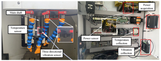
Figure 1.
Data acquisition system.
2.2. System Parameter Configuration and Data Collection
In CNC machining, processing conditions directly affect the material processing quality. The wear state of the tool depends on the type of material being processed and is influenced by the material hardness, toughness, friction characteristics, and processing conditions [21,22]. The workpiece used in this study was a rigid rectangular blank, as shown in Figure 2, The specific processing material parameters are shown in Table 1. The tool was a carbide end mill, with a diameter of 8 mm and four teeth. In addition, the machining process parameters play a key role [23]. For the CNC machine tool, the spindle speed was 4200 r/min, axial cutting depth was 0.8 mm, radial cutting depth was 4 mm, and feed speed was 500 mm/min. The sampling frequency of the three-way vibration signal was 4000 Hz, and the sampling frequency of the power and temperature signals was 10 Hz. These parameters are summarized in Table 2.
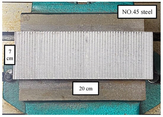
Figure 2.
Rigid rectangular blank workpiece.

Table 1.
Processing material parameters.
Table 2.
Processing parameter settings and signal recording conditions.
To ensure consistent sensor signals in the time domain during processing, the power and temperature signals from the same processing section were selected based on the time axis of the three-dimensional vibration signal. The sensor signal data are shown in Figure 3.
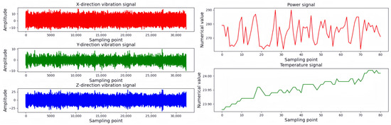
Figure 3.
Sensor signal data.
2.3. Classification of Tool-Wear Conditions
Tool wear results from intense friction between the workpiece, tool, and chip in the contact area, which leads to the gradual consumption of material on the front and rear faces of the tool. This wear reduces the cutting performance and processing efficiency of the tool. As wear on the tool surface is easy to observe and measure, the wear state is evaluated by measuring the wear width on the back face of the milling cutter using a high-precision electron microscope [24]. Extensive cutting experiments have shown that the wear process of the tool flank can be divided into three stages:
- Initial wear stage: The tool wears rapidly, but the amount of wear is limited. The main reason for this is the rapid removal of tiny uneven parts or oxide layers on the tool surface upon contact with the workpiece, which exposes a more stable tool material.
- Normal wear stage: Following the initial wear stage, the tool enters a phase where the wear rate stabilizes and increases linearly at a gradual rate. The cutting performance of the tool is stable during this stage, and this phase constitutes the longest portion of the tool’s service life.
- Severe wear stage: In the final stage of tool wear, the wear rate increases sharply, resulting in a rapid decrease in the cutting performance of the tool and ultimately leading to tool failure or chipping.
According to the GB/T 16460-2016 standard [25], the flank wear width (VB) is used as the basis for tool-wear-status classification. Specifically, a wear amount exceeding 0.1 mm is considered to correspond to a transition to the next wear state. Based on this threshold, the tool-wear state is categorized into three groups, as outlined in Table 3.
Table 3.
Degrees of tool wear.
Tool-wear-state data were collected through multiple continuous milling experiments and classified into the three wear states (initial wear, normal wear, and severe wear), as shown in Figure 4.
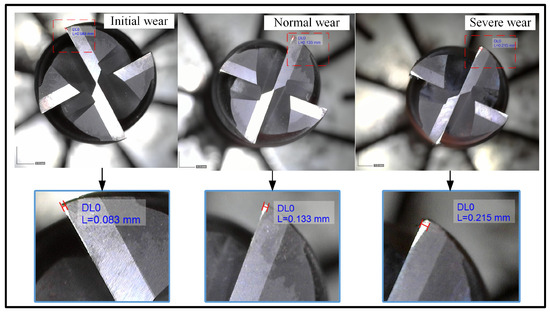
Figure 4.
Three types of wear states of cutting tools.
3. Multi-Domain Feature Extraction and Information Fusion
Multi-domain feature extraction involves time-domain, frequency-domain, and time–frequency-domain feature extraction. Features in different domains reflect the tool-wear status from different perspectives. Time-domain features capture the time-varying characteristics of the signal during tool wear; frequency-domain features identify the specific frequency characteristics associated with tool wear; and time–frequency-domain features capture the relationship between the signal frequency and time. Through multi-domain feature extraction, the characteristics related to the tool-wear state can be comprehensively captured. This study uses PCA to fuse multi-domain features. The fused features are then input to the tool-wear-state identification model to improve the accuracy of tool-wear-state identification.
3.1. Time-Domain Feature Extraction
Time-domain feature extraction involves calculating statistical features from the time series of a signal by analyzing changes in the signal amplitude over time. In tool processing, tools with different degrees of wear cause changes in the time-domain signal characteristics. The time-domain features selected in this study are listed in Table 4.
Table 4.
Time-domain features.
In Table 4, represents the time-domain data of the input signal; , where denotes the signal length; represents the dimensioned time-domain feature; and represents the dimensionless time-domain feature [19]. By comparing the variation trends in time-domain-feature indicators, the wear state of the tool can be comprehensively evaluated.
3.2. Frequency-Domain Feature Extraction
Frequency-domain features describe the energy distribution and frequency components of a signal at different frequencies. These features are obtained using Fourier transform, which converts a signal from the time domain to the frequency domain and then establishes the relationship between amplitude and phase with frequency as the independent variable. As this study focuses on discrete-time signals, the fast Fourier transform is used to convert the signal between the time and frequency domains. The power spectrum reflects the power distribution of the signal at each frequency. This study uses the autocorrelation function method to calculate the power spectrum of the signal. The computation can be expressed as follows:
where represents the time delay; represents the autocorrelation function of ; and represents the number of sampling points. The frequency-domain features selected in this study are listed in Table 5, where represents the frequency corresponding to the th spectrum.
Table 5.
Frequency-domain features.
3.3. Time–Frequency-Domain Feature Extraction
Time–frequency-domain characteristics can capture dynamic changes in the signal across both time and frequency domains, reflecting the time–frequency-domain characteristics of different tool-wear states through the wavelet-packet energy proportion . In this study, the db1 wavelet is used to decompose the signal into different wavelet packets. Each layer of wavelet packets contains nodes, where is the number of decomposition layers. The wavelet packet coefficients of different nodes are obtained through wavelet-packet decomposition. is the signal length of each node after wavelet-packet decomposition. The wavelet-packet energy proportion can be expressed as follows:
where represents the different nodes of the signal, and is the total energy of each node.
3.4. Multi-Sensor Feature Fusion Based on PCA
Multi-domain features from multi-sensor signals are combined into a feature vector, and the multi-domain feature matrix is then established based on multiple sets of data. To reduce the complexity of multi-domain feature matrices, PCA is used to fuse multi-domain feature matrices. PCA maps the feature matrix of multiple domains to a lower-dimensional space through linear transformation. This process ensures that the dimensionality of the feature matrix is reduced while retaining as much information as possible [26,27]. The first step in feature fusion based on PCA is to standardize the feature data:
where represents the feature of the multi-domain feature matrix; represents the standardized feature; and and denote the minimum and maximum values of the multi-domain feature matrix, respectively.
Subsequently, a new feature space is constructed as follows:
where is the covariance matrix of the feature matrix, and and denote the corresponding eigenvalues and eigenvectors, respectively. is the fused feature matrix, is the original feature matrix, and is the matrix composed of .
Lastly, the number of principal components (number of features after fusion), which represents the dimension of the feature vector, is determined according to the cumulative contribution rate of the principal component variance. When exceeds 95%, the number of corresponding fused features is the dimension of the final selected feature vector; can be expressed as follows:
where is the cumulative contribution rate of the first principal component features.
3.5. Multi-Domain Feature Extraction and Feature Fusion Experiment
For this study, 600 sets of initial-wear, normal-wear, and severe-wear data for the tool were collected. The specific division is presented in Table 6. Dataset collection involves the following steps: First, a microscope is used to obtain images of the tool wear after each processing step. Next, based on these images, the tools are classified according to Table 3, and each wear state is labelled. Lastly, to ensure the integrity and accuracy of the experimental data, the signal data collected by multiple sensors during each processing step are recorded, ensuring that each tool-wear image accurately corresponds to the relevant multi-sensor signal. This approach not only enhances the reliability of experimental data but also provides sufficient support for subsequent analysis.
Table 6.
Tool-wear-status dataset division.
A set of machining data is randomly selected for each tool-wear state. The time-domain characteristics of the vibration signal in the X direction are shown in Figure 5a; the frequency-domain power spectrum of the vibration signal in the Z direction is shown in Figure 5b; and the time–frequency-domain energy proportion of the three-layer wavelet packet decomposition of the vibration signal in the Y direction is shown in Figure 5c.
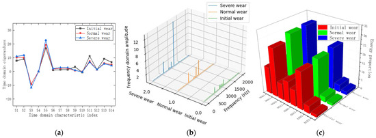
Figure 5.
Multi-domain feature extraction of three-way vibration signals. (a) Time-domain feature comparison; (b) frequency-domain feature comparison; (c) comparison of time–frequency-domain characteristics.
Figure 5 shows that multi-domain feature extraction from vibration signals in the X, Y, and Z directions effectively reflects the tool characteristics under different wear states. However, as is shown in Figure 5a, the time-domain eigenvalues of S4, S10, and S12 for the three wear states are approximately equal. Figure 5b shows that the power spectra of the three wear states exhibit no obvious feature contrast between 500 Hz and 1000 Hz. Figure 5c shows that the energy proportions of the AAA3 node are approximately equal. These outcomes verify the presence of redundant data in multi-domain feature extraction. These redundant features not only increase the complexity of data processing and analysis but also affect the accuracy of tool-wear identification.
As the sampling frequencies of the power and temperature signals are both 10 Hz, only their time-domain features are extracted, as shown in Figure 6.
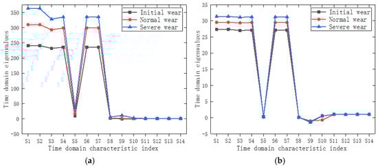
Figure 6.
Time-domain feature comparison. (a) Comparison of power time-domain characteristics; (b) comparison of temperature time-domain characteristics.
Figure 6 shows that in the time-domain characteristics of the power and temperature signals, the eigenvalues of S5, S8, S11, S12, S13, and S14 of the three tool-wear states are approximately equal, indicating feature redundancy. However, other time-domain feature indicators clearly distinguish the wear states of different tools.
To address feature redundancy, the multi-domain features from the three-way vibration, power, and temperature signals are combined into a feature vector. For the vibration signals, there are 14 time-domain features, four frequency-domain features, and eight time–frequency-domain features in each direction (X, Y, and Z). Therefore, a total of 3 × (14 + 4 + 8) = 78 three-way vibration signals are extracted. For the power and temperature signals, there are 14 time-domain features each, resulting in a 1 × 10⁶ multi-domain feature vector.
In this study, 600 sets of data for the three tool-wear states are extracted. According to the multi-domain feature vector dimension, the 600 sets of data are combined into a 600 × 106 feature matrix, with each row of the matrix representing the tool-wear state of a sample. The feature matrix is fused based on the PCA method. Figure 7 shows the cumulative contribution rates of the principal components of the PCA fusion feature.
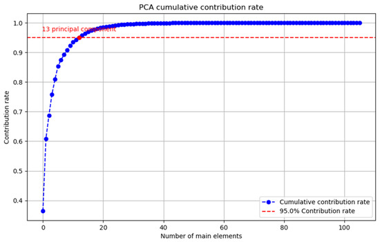
Figure 7.
Feature fusion.
When the cumulative contribution rate is 95%, the number of principal components is 13, and the dimension of the feature matrix is 600 × 13. This confirms that PCA effectively mitigates redundant features, reduces the dimension of the feature matrix, and retains the key features with a strong ability to recognize tool-wear status.
4. The SSA–BP Neural Network Model for Tool-State Identification
4.1. BP Neural Network
The BP neural network exhibits excellent organization and adaptability. Through sample learning, nonlinear problems can be solved, and the mapping relationship between multi-domain features and tool-wear status can be identified [28,29,30]. The BP neural network consists of three parts: an input layer, a hidden layer, and an output layer. In the BP neural network established in this study, a 600 × 13 feature matrix obtained after PCA feature fusion serves as the input layer. Thus, the number of neurons is 13. The hidden layer uses empirical methods, and the number of neurons is 7. The output layer represents the three tool-wear states, namely initial wear, normal wear, and severe wear, and thus, the number of neurons is 3. The basic structure of the BP neural network is shown in Figure 8.
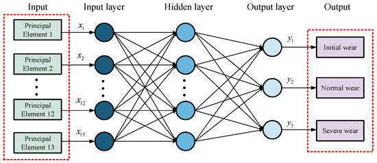
Figure 8.
BP neural network structure.
In training the BP neural network, the network parameters are adjusted through training data to minimize the output error. This process involves two stages: forward propagation of information and backpropagation of error. In the first stage, input data are fed to the input layer and propagate through the hidden layers in a layer-by-layer manner to the output layer. In each layer, after the neurons receive the input signal, they perform weighted and activation functions and then pass the output to the neurons in the next layer. In the second stage, the error between the output and expected results is calculated using the cross-entropy loss function. According to the error, the weights and thresholds between each neuron are adjusted through the BP algorithm to reduce the error between the output and expected results. Multiple iterations of forward propagation and backpropagation are performed until the error is minimized.
4.2. Mahjong Search Algorithm
The SSA is an optimization algorithm based on the foraging and anti-predator behaviors of sparrows [31]. In the SSA, each sparrow exhibits one of three behaviors: (1) discoverer, looking for food; (2) follower, relying on the finder to locate food; and (3) sentinel, detecting danger and deciding whether to continue foraging [32].
The position update strategy of each individual varies according to its role in the population. The main task of the discoverer is to find potential food resources. To explore the surrounding environment, the discoverer uses a large step size and randomness to avoid local optimal solutions and search for the global optimal solution in a wide space. The position update strategy of the discoverer can be expressed as follows:
where is the maximum number of iterations; is the current iteration; ; represents the next value of the th sparrow at the th iteration; is a random number between 0 and 1, (alarm value) is a number ranging from 0 to 1; is the safety threshold ranging between 0.5 and 1; is a random number based on normal distribution; and represents a matrix, where each element is 1. If , the discoverer is considered to have perceived a predator, and all sparrows must rapidly fly to safe areas. Conversely, if , no predators are around, and the discoverer enters a wide search mode.
The follower mainly relies on the information provided by the discoverer to locate food resources. Its position update strategy is more conservative to ensure that it can stably follow the discoverer, and this strategy can be expressed as follows:
where is the best position of the discoverer; represents the current global worst position; and represents a matrix that randomly assigns each element a value of 1 or −1, with . If , followers with poorer fitness values are less likely to follow the discoverer.
The sentinels are responsible for identifying potential dangers and alerting the population. The initial positions of these sentinels are randomly generated, and their position update strategy is conservative to avoid dangers and ensure alertness. The position update strategy of the sentinels can be expressed as follows:
where is the current global optimal position; is a small constant; is a random number that follows a standard normal distribution; and are the current global best and worst fitness values respectively; −1 < k < 1 is a random number; and is the fitness value of the current sparrow. means that the sparrow in the middle of the population is aware of the danger and should move closer to the other sparrows. If , the sparrow is at the edge of the population.
4.3. The SSA–BP Neural Network Identification Model
Although the BP network exhibits a strong local optimization ability, it is vulnerable to the initial weights and thresholds of neurons and may fall into local optimality. Therefore, the SSA is used to optimize the initial weights and thresholds of the BP neural network to improve the identification accuracy of the tool-wear state [33,34,35]. The SSA–BP optimization process is summarized in Table 7.
Table 7.
SSA–BP neural network identification model.
5. Experimental Verification of Tool-Wear-State Identification
The CNC machine model used in this experiment is XK-7132 (Shandong Weida Heavy Industry Co., Ltd., Tengzhou, China). According to the tool-wear status (Table 3), the collected data are labelled and classified, as indicated in Table 6. The activation functions in the hidden and output layers of the SSA–BP neural network are the rectified linear unit and Softmax functions, respectively. The learning rate is 0.001, and the number of iterations is 1000. The sparrow population size is set as 20, the number of iterations is 50, the proportion of discoverers is 0.2, the proportion of sentinels is 0.1, and is 0.8. In the experiment, 80% of the data for each tool-wear state were used for model training, and the remaining 20% were used for model testing. Therefore, the training and test sets include 480 and 120 groups, respectively. Figure 9 shows the best fitness curve for the SSA-optimized BP neural network. The model attains the best fitness and achieves the optimal thresholds and weights by the 16th iteration.
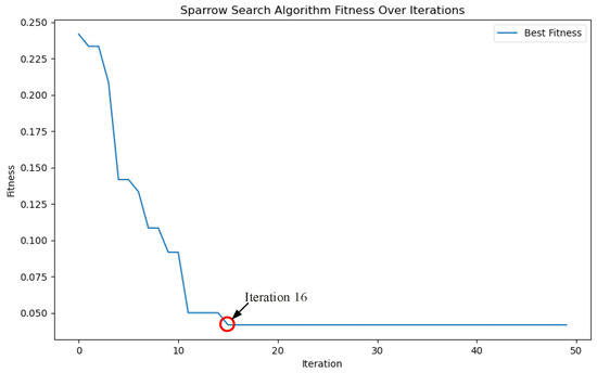
Figure 9.
Population evolution curve.
Figure 10 shows the iteration epochs of the SSA–BP neural network model. The dynamic evolutions of the training and test sets of the SSA–BP neural network model follow a consistent pattern. Therefore, the proposed model can accurately identify the tool-wear state.
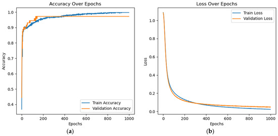
Figure 10.
Iteration epochs of SSA–BP neural network model. (a) Accuracy over epochs; (b) loss over epochs.
To demonstrate the superiority of the proposed method, it is compared with the k-nearest neighbors (KNN), support vector machine (SVM), and BP neural network models [36,37,38]. In terms of identification errors, Figure 11a shows that the KNN model incurs four errors in the initial-wear state, two errors in the normal-wear state, and two errors in the severe-wear state. Figure 11b shows that the SVM model yields three errors in the initial-wear state, two errors in the normal-wear state, and two errors in the severe-wear state. Figure 11c shows that the BP neural network model has one error in the initial-wear state, two errors in the normal-wear state, and one error in the severe-wear state. Figure 11d shows that the SSA–BP neural network model has one error in the initial-wear state, none in the normal-wear state, and one error in the severe-wear state. These results validate that the SSA–BP neural network model achieves a higher identification accuracy than the SVM, KNN, and BP neural network models.
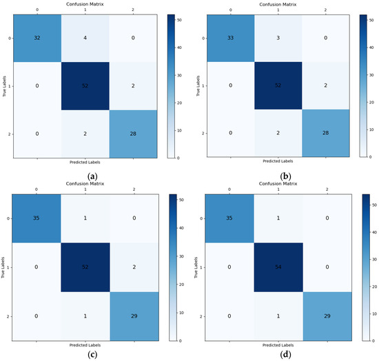
Figure 11.
Confusion matrix for four models: (a) KNN; (b) SVM; (c) BP neural network; (d) SSA–BP neural network.
As is shown in Figure 11, the KNN model, whose performance is significantly affected by noise and outliers, exhibits the lowest accuracy in tool-wear identification. The SVM model, which is characterized by a significant computational overhead on large datasets, especially in high-dimensional spaces, exhibits low identification accuracy. Although the BP neural network can capture complex nonlinear relationships, it is prone to overfitting and falling into local optimality. In contrast, the SSA–BP model can adaptively optimize parameters by leveraging the SSA algorithm when processing complex and noisy large-scale data, avoiding the model falling into local optimality and improved tool-wear identification accuracy.
To quantitatively analyze the identification performance of the four models, accuracy, precision, recall rate, and the F1 score are used as evaluation indicators. The evaluation indicators are defined as follows:
where represents the number of positive cases correctly identified, denotes the number of negative cases correctly identified, represents the number of positive cases incorrectly identified, and represents the number of negative cases incorrectly identified.
These four indicators can not only comprehensively reflect the accuracy of tool-wear-status identification, but also effectively assess the identification efficiency and reliability. Table 8 presents a comparison of the performance of different models in terms of tool-wear-state identification.
Table 8.
Performance-indicator comparison results of different models.
The differences in model performance can be comprehensively assessed based on the accuracy, precision, recall, and F1 score. For a more intuitive visualization, Figure 12 illustrates the performance indicators of different models.
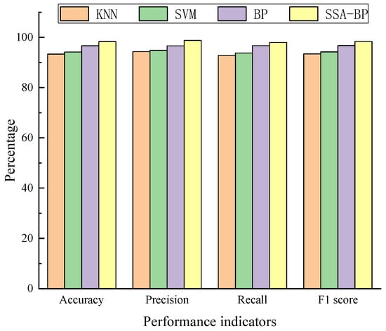
Figure 12.
Model performance indicator comparison.
Table 8 indicates that the BP neural network model outperforms the KNN and SVM models owing to its strong nonlinear mapping and adaptive learning abilities. In addition, the SSA–BP neural network model exhibits an accuracy of 98.33%, a precision of 98.81%, a recall of 97.96%, and an F1 score of 98.36%, all exceeding those of the KNN, SVM, and BP neural network models. These results further confirm the effectiveness of the proposed method.
Overall, the experimental results indicate that the performance indicators of the proposed SSA–BP model are superior to those of the KNN, SVM, and BP neural network models. The accuracy, precision, recall, and F1 score were 98.33%, 98.81%, 97.96%, and 98.36%, respectively, and the identification errors were minimal. Only one error was observed in both the initial-wear and severe-wear conditions, and no errors were incurred in the normal-wear condition. Therefore, the proposed model can accurately identify the tool-wear state.
6. Conclusions
This paper proposes a tool-wear-state identification method based on information fusion and the SSA–BP neural network. First, a multi-sensor signal acquisition system was established, and multi-domain features of multi-sensor signals were extracted. Second, the multi-domain features of three-way vibration, power, and temperature signals were fused. Finally, the SSA was used to optimize the neuron weights and thresholds of the BP neural network, and the SSA–BP model was constructed and verified. The following conclusions are derived:
- The proposed method comprehensively captures the key characteristics of tool wear by fusing the multi-domain features of three-way vibration, power, and temperature signals. The advantages of multiple signals were leveraged to ensure comprehensive and accurate identification of tool-wear status.
- PCA effectively reduces the redundant features in the data and retains the features essential to the identification of tool-wear status. This approach reduces the computational complexity and improves the overall performance of the system.
- The neuron weights and thresholds of the BP neural network were optimized using the SSA algorithm, addressing the risk of the BP neural network falling into the local optima. SSA optimization enhances the stability of the neural network training process and improves the accuracy of tool-wear-state identification.
- The proposed method achieved an identification accuracy of 98.33%, a precision of 98.81%, a recall of 97.96%, and an F1 score of 98.36%. These results highlight the potential of the proposed method to efficiently and accurately identify the tool-wear state in practical applications.
Future research could aim to refine tool-wear classification based on the surface accuracy of the processed material and to clarify the influence of tool-wear status on processing accuracy. Moreover, the incorporation of additional sensor signals, such as the cutting force and cutting-edge temperature, could supplement the dataset and improve the accuracy of tool-wear-status identification.
Author Contributions
Methodology, X.G.; software, S.L.; validation, T.D.; writing—original draft preparation, Z.W.; writing—review and editing, H.C. All authors have read and agreed to the published version of the manuscript.
Funding
This research was funded by the Jilin Provincial Science and Technology Development Plan Project (Grant No. YDZJ202401615ZYTS) and the Jilin Provincial Science and Technology Department Key Research and Development Project (Grant No. 20220201156GX).
Data Availability Statement
Data underlying the results presented in the paper are not publicly available at this time but may be obtained from the authors upon reasonable request.
Conflicts of Interest
The authors declare no conflicts of interest.
References
- del Olmo, A.; de Lacalle, L.N.L.; de Pissón, G.M.; Pérez-Salinas, C.; Ealo, J.A.; Sastoque, L.; Fernandes, M.H. Tool wear monitoring of high-speed broaching process with carbide tools to reduce production errors. Mech. Syst. Signal Process. 2022, 172, 109003. [Google Scholar] [CrossRef]
- Cheng, Y.N.; Gai, X.Y.; Guan, R.; Jin, Y.B.; Lu, M.D.; Ding, Y. Tool wear intelligent monitoring techniques in cutting: A review. J. Mech. Sci. Technol. 2023, 37, 289–303. [Google Scholar] [CrossRef]
- Zhou, Q.; Yan, P.; Liu, H.Y.; Xin, Y.; Chen, Y.Z. Research on a configurable method for fault diagnosis knowledge of machine tools and its application. Int. J. Adv. Manuf. Technol. 2018, 95, 937–960. [Google Scholar] [CrossRef]
- Liu, B.; Li, H.K.; Ou, J.Y.; Wang, Z.D.; Sun, W. Intelligent recognition of milling tool wear status based on variational auto-encoder and extreme learning machine. Int. J. Adv. Manuf. Technol. 2022, 119, 4109–4123. [Google Scholar] [CrossRef]
- Hassan, M.; Sadek, A.; Attia, M.H. Novel sensor-based tool wear monitoring approach for seamless implementation in high speed milling applications. CIRP Ann.-Manuf. Technol. 2021, 70, 87–90. [Google Scholar] [CrossRef]
- Jaini, S.N.B.; Lee, D.W.; Lee, S.J.; Kim, M.R.; Son, G.H. Indirect tool monitoring in drilling based on gap sensor signal and multilayer perceptron feed forward neural network. J. Intell. Manuf. 2021, 32, 1605–1619. [Google Scholar] [CrossRef]
- Wang, G.F.; Yang, Y.W.; Zhang, Y.C.; Xie, Q.L. Vibration sensor based tool condition monitoring using ν support vector machine and locality preserving projection. Sens. Actuators A-Phys. 2014, 209, 24–32. [Google Scholar] [CrossRef]
- Chen, B.X.; Chen, Y.C.; Lon, C.H.; Chou, Y.C.; Wang, F.C.; Su, W.Z. Application of Generative Adversarial Network and Diverse Feature Extraction Methods to Enhance Classification Accuracy of Tool-Wear Status. Electronics 2022, 11, 2364. [Google Scholar] [CrossRef]
- Aldekoa, I.; del Olmo, A.; Sastoque-Pinilla, L.; Sendino-Mouliet, S.; Lopez-Novoa, U.; de Lacalle, L.N.L. Early detection of tool wear in electromechanical broaching machines by monitoring main stroke servomotors. Mech. Syst. Signal Process. 2023, 204, 110773. [Google Scholar] [CrossRef]
- Zhang, Y.P.; Qi, X.Z.; Wang, T.; He, Y.H. Tool Wear Condition Monitoring Method Based on Deep Learning with Force Signals. Sensors 2023, 23, 4595. [Google Scholar] [CrossRef]
- Wang, C.D.; Bao, Z.K.; Zhang, P.D.; Ming, W.W.; Chen, M. Tool wear evaluation under minimum quantity lubrication by clustering energy of acoustic emission burst signals. Measurement 2019, 138, 256–265. [Google Scholar] [CrossRef]
- Kong, L.B.; Peng, X.; Chen, Y.; Wang, P.; Xu, M. Multi-sensor measurement and data fusion technology for manufacturing process monitoring: A literature review. Int. J. Extrem. Manuf. 2020, 2, 022001. [Google Scholar] [CrossRef]
- Kuntoglu, M.; Salur, E.; Gupta, M.K.; Sarikaya, M.; Pimenov, D.Y. A state-of-the-art review on sensors and signal processing systems in mechanical machining processes. Int. J. Adv. Manuf. Technol. 2021, 116, 2711–2735. [Google Scholar] [CrossRef]
- Huang, J.S.; Chen, G.J.; Wei, H.; Chen, Z.; Lv, Y.X. Sensor-based intelligent tool online monitoring technology: Applications and progress. Meas. Sci. Technol. 2024, 35, 112001. [Google Scholar] [CrossRef]
- Tang, K.E.; Huang, Y.C.; Liu, C.W. Development of multi-sensor data fusion and in-process expert system for monitoring precision in thin wall lens barrel turning. Mech. Syst. Signal Process. 2024, 210, 111195. [Google Scholar] [CrossRef]
- Gomes, M.C.; Brito, L.C.; da Silva, M.B.; Duarte, M.A.V. Tool wear monitoring in micromilling using Support Vector Machine with vibration and sound sensors. Precis. Eng.-J. Int. Soc. Precis. Eng. Nanotechnol. 2021, 67, 137–151. [Google Scholar] [CrossRef]
- Gao, K.P.; Xu, X.X.; Jiao, S.J. Measurement and prediction of wear volume of the tool in nonlinear degradation process based on multi-sensor information fusion. Eng. Fail. Anal. 2022, 136, 106164. [Google Scholar] [CrossRef]
- Niaki, F.A.; Feng, L.; Ulutan, D.; Mears, L. A wavelet-based data-driven modelling for tool wear assessment of difficult to machine materials. Int. J. Mechatron. Manuf. Syst. 2016, 9, 97–121. [Google Scholar] [CrossRef]
- Ni, J.; Liu, X.S.; Meng, Z.; Cui, Y.M. Identification of Tool Wear Based on Infographics and a Double-Attention Network. Machines 2023, 11, 927. [Google Scholar] [CrossRef]
- Xu, Y.W.; Gui, L.; Xie, T.C. Intelligent Recognition Method of Turning Tool Wear State Based on Information Fusion Technology and BP Neural Network. Shock Vib. 2021, 2021, 7610884. [Google Scholar] [CrossRef]
- Fernández-Abia, A.I.; Barreiro, J.; de Lacalle, L.N.L.; Martínez-Pellitero, S. Behavior of austenitic stainless steels at high speed turning using specific force coefficients. Int. J. Adv. Manuf. Technol. 2012, 62, 505–515. [Google Scholar]
- Amigo, F.J.; Urbikain, G.; Pereira, O.; Fernández-Lucio, P.; Fernández-Valdivielso, A.; de Lacalle, L.N.L. Combination of high feed turning with cryogenic cooling on Haynes 263 and Inconel 718 superalloys. J. Manuf. Process. 2020, 58, 208–222. [Google Scholar]
- Peña, B.; Aramendi, G.; Rivero, A.; de Lacalle, L.N.L. Monitoring of drilling for burr detection using spindle torque. Int. J. Mach. Tools Manuf. 2005, 45, 1614–1621. [Google Scholar] [CrossRef]
- Junge, T.; Liborius, H.; Mehner, T.; Nestler, A.; Schubert, A.; Lampke, T. Measurement system based on the Seebeck effect for the determination of temperature and tool wear during turning of aluminum alloys. Procedia CIRP 2020, 93, 1435–1441. [Google Scholar] [CrossRef]
- Duan, J.; Liang, J.Q.; Yu, X.J.; Si, Y.; Zhang, X.B.; Shi, T.L. Toward practical tool wear prediction paradigm with optimized regressive Siamese neural network. Adv. Eng. Inform. 2023, 58, 102200. [Google Scholar] [CrossRef]
- Alkhayrat, M.; Aljnidi, M.; Aljoumaa, K. A comparative dimensionality reduction study in telecom customer segmentation using deep learning and PCA. J. Big Data 2020, 7, 9. [Google Scholar]
- Marukatat, S. Tutorial on PCA and approximate PCA and approximate kernel PCA. Artif. Intell. Rev. 2023, 56, 5445–5477. [Google Scholar]
- Wang, D.S.; Hong, R.J.; Lin, X.C. A method for predicting hobbing tool wear based on CNC real-time monitoring data and deep learning. Precis. Eng.-J. Int. Soc. Precis. Eng. Nanotechnol. 2021, 72, 847–857. [Google Scholar]
- Li, J.; Zhao, J.T.; Liu, Q.H.; Zhu, L.Z.; Guo, J.Y.; Zhang, W.J. Optimization of CNC Turning Machining Parameters Based on Bp-DWMOPSO Algorithm. Cmc-Comput. Mater. Contin. 2023, 77, 223–244. [Google Scholar]
- Cao, Y.X.; Zhao, J.; Qu, X.T.; Wang, X.; Liu, B.W. Prediction of Abrasive Belt Wear Based on BP Neural Network. Machines 2021, 9, 314. [Google Scholar] [CrossRef]
- Xue, J.K.; Shen, B. A survey on sparrow search algorithms and their applications. Int. J. Syst. Sci. 2024, 55, 814–832. [Google Scholar]
- Yue, Y.G.; Cao, L.; Lu, D.W.; Hu, Z.Y.; Xu, M.H.; Wang, S.X.; Li, B.; Ding, H.H. Review and empirical analysis of sparrow search algorithm. Artif. Intell. Rev. 2023, 56, 10867–10919. [Google Scholar]
- Li, M.H.; Gu, Y.L.; Ge, S.K.; Zhang, Y.F.; Mou, C.; Zhu, H.C.; Wei, G.F. Classification and identification of mixed gases based on the combination of semiconductor sensor array with SSA-BP neural network. Meas. Sci. Technol. 2023, 34, 085110. [Google Scholar] [CrossRef]
- Wang, J.L.; Zeng, G.R.; Xu, M.S.; Wan, X.C.; Wang, K.K.; Mou, J.G.; Hua, C.C.; Fan, C.H.; Han, P.F. SSA-BP Neural Network Model for Predicting Rice-Fish Production in China. J. Appl. Ichthyol. 2024, 2024, 5739961. [Google Scholar]
- Wang, J.; Chen, B.C.; Yang, W.S.; Xu, D.; Yan, B.; Zou, E.D. BP neural network multi-module green roof thermal performance prediction model optimized based on sparrow search algorithm. J. Build. Eng. 2024, 96, 110615. [Google Scholar]
- Vommi, A.M.; Battula, T.K. A hybrid filter-wrapper feature selection using Fuzzy KNN based on Bonferroni mean for medical datasets classification: A COVID-19 case study. Expert Syst. Appl. 2023, 219, 119612. [Google Scholar]
- Kareem, I.; Ali, S.F.; Bilal, M.; Hanif, M.S. Exploiting the features of deep residual network with SVM classifier for human posture recognition. PLoS ONE 2024, 19, e0314959. [Google Scholar]
- Liang, R.; Wang, P.H.; Hu, L.H. Application of Visual Recognition Based on BP Neural Network in Architectural Design Optimization. Comput. Intell. Neurosci. 2022, 2022, 3351196. [Google Scholar]
Disclaimer/Publisher’s Note: The statements, opinions and data contained in all publications are solely those of the individual author(s) and contributor(s) and not of MDPI and/or the editor(s). MDPI and/or the editor(s) disclaim responsibility for any injury to people or property resulting from any ideas, methods, instructions or products referred to in the content. |
© 2025 by the authors. Licensee MDPI, Basel, Switzerland. This article is an open access article distributed under the terms and conditions of the Creative Commons Attribution (CC BY) license (https://creativecommons.org/licenses/by/4.0/).