1. Introduction
During CNC machine tool cutting, the tool-wear state directly affects the surface quality, processing efficiency, and processing accuracy of the workpiece [
1,
2]. Approximately 20% of CNC machine tool failures are attributable to tool wear [
3]. Hence, identification of the tool-wear status is the focus of extensive attention from engineers and scholars. Tool-wear identification methods can be divided into direct and indirect approaches [
4]. Direct methods require halting CNC machine tool operations to capture images of the worn tool using charge-coupled-device cameras and lighting units. The tool-wear state is then identified from the images. However, this approach reduces the workpiece processing efficiency. In indirect methods, sensors such as vibration, cutting-force, acoustic-emission, and current sensors are installed in the CNC machine tool, and the tool-wear status is analyzed using the signals of various sensors [
5,
6]. This method can identify the tool-wear status without interrupting the machining process, while reducing the complexity of detection operations. Therefore, at present, tool-wear-state identification is mainly based on indirect methods.
In recent years, numerous scholars have explored indirect methods for identifying tool-wear status. Wang et al. [
7] collected vibration signals during workpiece machining and used a support vector machine (SVM) to identify the tool-wear status. Chen et al. [
8] performed linear interpolation on vibration signals to improve the data integrity and used the complete vibration signal data to construct a tool-wear-state identification model based on a convolutional neural network. Aldekoa et al. [
9] analyzed the correlation between the servo motor variables and the tool status of a broaching machine, and used a regression machine learning algorithm to effectively predict the tool-wear status. Zhang et al. [
10] constructed a convolutional neural network model with multi-scale features based on the cutting-force signals extracted during machining, thereby improving the accuracy of tool-wear-state identification. Wang et al. [
11] used the clustering energy of acoustic-emission burst signals to evaluate the tool-wear state through a linear fitting method.
Notably, in these methods, the signal information provided by a single sensor indicates only a single physical quantity, which limits enhancement of the accuracy of tool-wear identification. Multi-sensor information fusion technology can fully leverage the complementary advantages of multiple sensor signals, ensure the reliability and comprehensiveness of the monitoring signals, and improve the accuracy of tool-wear-status identification [
12,
13,
14,
15]. For tool-wear-state identification, Gomes et al. [
16] combined vibration and acoustic-emission signals to identify the most relevant features of tool wear using recursive feature elimination and SVM. Gao et al. [
17] collected three-dimensional vibration signals, three-dimensional force signals, and acoustic-emission signals during workpiece processing and performed multi-sensor, mixed-field-feature information fusion. Additionally, deep neural networks were incorporated to identify the tool-wear status. Niaki et al. [
18] performed feature fusion on power and vibration signals based on principal component analysis (PCA) to eliminate redundant and irrelevant feature data and designed a neural network with Bayesian regularization to improve the accuracy of tool-wear-state identification. Ni et al. [
19] used vibration and acoustic-emission signals for multi-domain feature fusion and proposed a dual-attention model based on information graphs to identify the tool-wear state. Xu et al. [
20] developed a wavelet-packet-decomposition method to extract the optimal characteristic frequency bands of acoustic-emission and vibration-acceleration signals, and combined it with a backpropagation (BP) neural network to identify the tool-wear status.
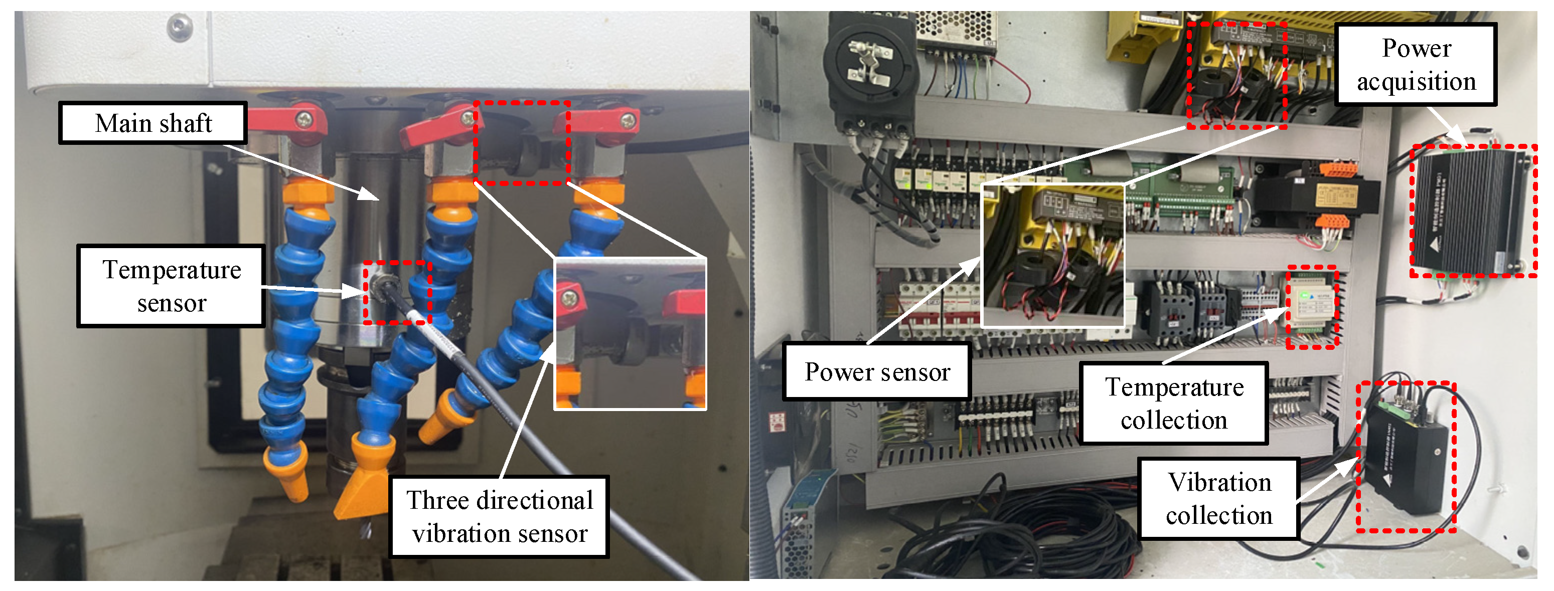
Based on this review, a comprehensive evaluation is performed that considers the cost, installation mode, environmental adaptability, and measurement accuracy. For this study, three-way vibration signals, power signals, and temperature signals are selected as the primary data for tool-wear-state identification. The three-way vibration signal, which is closely related to the dynamic characteristics of the process system (including the tool, machine tool, fixture, and workpiece), can effectively reflect the dynamic changes induced by tool wear. The power signal exhibits significant amplitude variation and is robust against disturbances induced by chips and coolant. The temperature signal reflects the friction heat generated during tool wear and can indirectly reflect the degree of wear. The combination of these signals can compensate for the limitations of individual signals and enhance the accuracy and reliability of tool-wear-status identification through multi-dimensional information fusion.
Based on the PCA, this study integrates multi-domain feature information from three-way vibration signals, power signals, and temperature signals collected during a CNC milling process. This integration reduces feature dimensionality and data complexity. To address the limitations of the BP neural network, i.e., its vulnerability to initial weights and thresholds, which may lead to it falling into local optima, it is integrated with the sparrow search algorithm (SSA) to establish an SSA–BP model. Specifically, the SSA optimizes the initial threshold and weight of the BP neural network to enhance the identification accuracy of the tool state.
3. Multi-Domain Feature Extraction and Information Fusion
Multi-domain feature extraction involves time-domain, frequency-domain, and time–frequency-domain feature extraction. Features in different domains reflect the tool-wear status from different perspectives. Time-domain features capture the time-varying characteristics of the signal during tool wear; frequency-domain features identify the specific frequency characteristics associated with tool wear; and time–frequency-domain features capture the relationship between the signal frequency and time. Through multi-domain feature extraction, the characteristics related to the tool-wear state can be comprehensively captured. This study uses PCA to fuse multi-domain features. The fused features are then input to the tool-wear-state identification model to improve the accuracy of tool-wear-state identification.
3.1. Time-Domain Feature Extraction
Time-domain feature extraction involves calculating statistical features from the time series of a signal by analyzing changes in the signal amplitude over time. In tool processing, tools with different degrees of wear cause changes in the time-domain signal characteristics. The time-domain features selected in this study are listed in
Table 4.
In
Table 4,
represents the time-domain data of the input signal;
, where
denotes the signal length;
represents the dimensioned time-domain feature; and
represents the dimensionless time-domain feature [
19]. By comparing the variation trends in time-domain-feature indicators, the wear state of the tool can be comprehensively evaluated.
3.2. Frequency-Domain Feature Extraction
Frequency-domain features describe the energy distribution and frequency components of a signal at different frequencies. These features are obtained using Fourier transform, which converts a signal from the time domain to the frequency domain and then establishes the relationship between amplitude and phase with frequency as the independent variable. As this study focuses on discrete-time signals, the fast Fourier transform is used to convert the signal between the time and frequency domains. The power spectrum reflects the power distribution of the signal at each frequency. This study uses the autocorrelation function method to calculate the power spectrum
of the signal. The computation can be expressed as follows:
where
represents the time delay;
represents the autocorrelation function of
; and
represents the number of sampling points. The frequency-domain features selected in this study are listed in
Table 5, where
represents the frequency corresponding to the
th spectrum.
3.3. Time–Frequency-Domain Feature Extraction
Time–frequency-domain characteristics can capture dynamic changes in the signal across both time and frequency domains, reflecting the time–frequency-domain characteristics of different tool-wear states through the wavelet-packet energy proportion
. In this study, the db1 wavelet is used to decompose the signal into different wavelet packets. Each layer of wavelet packets contains
nodes, where
is the number of decomposition layers. The wavelet packet coefficients
of different nodes are obtained through wavelet-packet decomposition.
is the signal length of each node after wavelet-packet decomposition. The wavelet-packet energy proportion
can be expressed as follows:
where
represents the different nodes of the signal, and
is the total energy of each node.
3.4. Multi-Sensor Feature Fusion Based on PCA
Multi-domain features from multi-sensor signals are combined into a feature vector, and the multi-domain feature matrix
is then established based on multiple sets of data. To reduce the complexity of multi-domain feature matrices, PCA is used to fuse multi-domain feature matrices. PCA maps the feature matrix of multiple domains to a lower-dimensional space through linear transformation. This process ensures that the dimensionality of the feature matrix is reduced while retaining as much information as possible [
26,
27]. The first step in feature fusion based on PCA is to standardize the feature data:
where
represents the feature of the multi-domain feature matrix;
represents the standardized feature; and
and
denote the minimum and maximum values of the multi-domain feature matrix, respectively.
Subsequently, a new feature space is constructed as follows:
where
is the covariance matrix of the feature matrix, and
and
denote the corresponding eigenvalues and eigenvectors, respectively.
is the fused feature matrix,
is the original feature matrix, and
is the matrix composed of
.
Lastly, the number of principal components (number of features after fusion), which represents the dimension of the feature vector, is determined according to the cumulative contribution rate
of the principal component variance. When
exceeds 95%, the number of corresponding fused features is the dimension of the final selected feature vector;
can be expressed as follows:
where
is the cumulative contribution rate of the first
principal component features.
3.5. Multi-Domain Feature Extraction and Feature Fusion Experiment
For this study, 600 sets of initial-wear, normal-wear, and severe-wear data for the tool were collected. The specific division is presented in
Table 6. Dataset collection involves the following steps: First, a microscope is used to obtain images of the tool wear after each processing step. Next, based on these images, the tools are classified according to
Table 3, and each wear state is labelled. Lastly, to ensure the integrity and accuracy of the experimental data, the signal data collected by multiple sensors during each processing step are recorded, ensuring that each tool-wear image accurately corresponds to the relevant multi-sensor signal. This approach not only enhances the reliability of experimental data but also provides sufficient support for subsequent analysis.
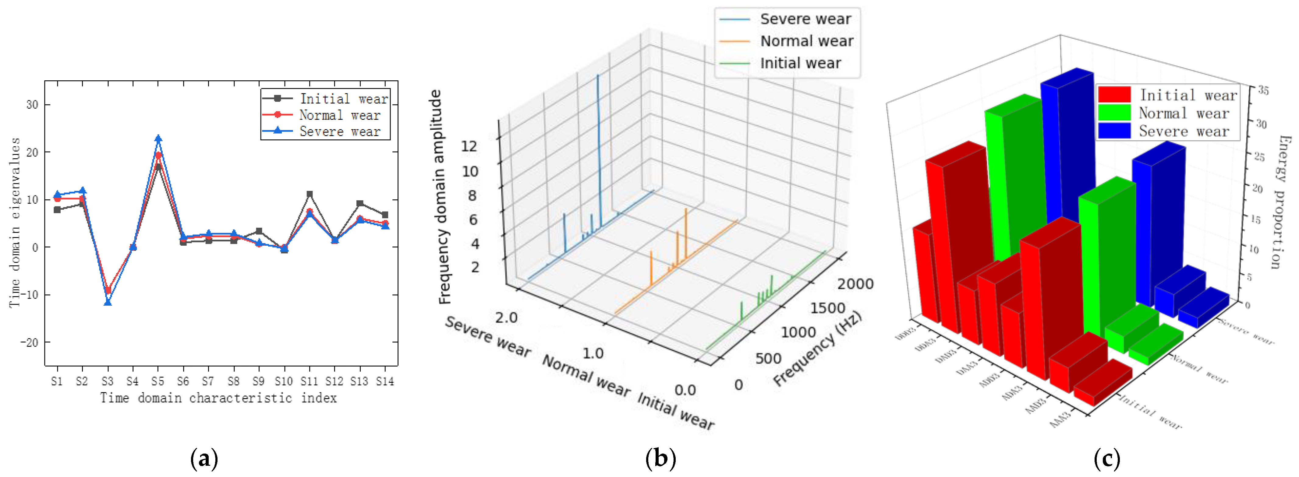
A set of machining data is randomly selected for each tool-wear state. The time-domain characteristics of the vibration signal in the
X direction are shown in
Figure 5a; the frequency-domain power spectrum of the vibration signal in the
Z direction is shown in
Figure 5b; and the time–frequency-domain energy proportion of the three-layer wavelet packet decomposition of the vibration signal in the
Y direction is shown in
Figure 5c.
Figure 5 shows that multi-domain feature extraction from vibration signals in the
X,
Y, and
Z directions effectively reflects the tool characteristics under different wear states. However, as is shown in
Figure 5a, the time-domain eigenvalues of S4, S10, and S12 for the three wear states are approximately equal.
Figure 5b shows that the power spectra of the three wear states exhibit no obvious feature contrast between 500 Hz and 1000 Hz.
Figure 5c shows that the energy proportions of the AAA3 node are approximately equal. These outcomes verify the presence of redundant data in multi-domain feature extraction. These redundant features not only increase the complexity of data processing and analysis but also affect the accuracy of tool-wear identification.
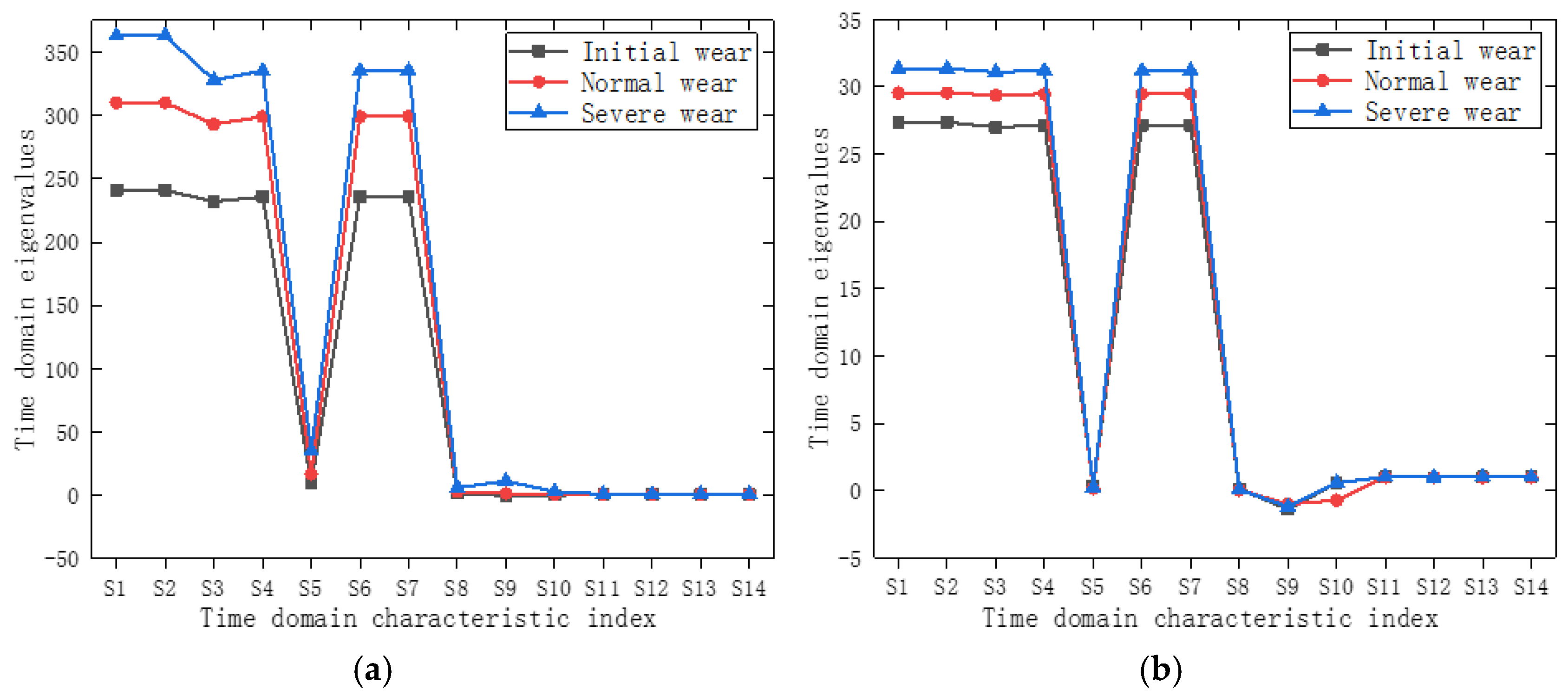
As the sampling frequencies of the power and temperature signals are both 10 Hz, only their time-domain features are extracted, as shown in
Figure 6.
Figure 6 shows that in the time-domain characteristics of the power and temperature signals, the eigenvalues of S5, S8, S11, S12, S13, and S14 of the three tool-wear states are approximately equal, indicating feature redundancy. However, other time-domain feature indicators clearly distinguish the wear states of different tools.
To address feature redundancy, the multi-domain features from the three-way vibration, power, and temperature signals are combined into a feature vector. For the vibration signals, there are 14 time-domain features, four frequency-domain features, and eight time–frequency-domain features in each direction (X, Y, and Z). Therefore, a total of 3 × (14 + 4 + 8) = 78 three-way vibration signals are extracted. For the power and temperature signals, there are 14 time-domain features each, resulting in a 1 × 10⁶ multi-domain feature vector.
In this study, 600 sets of data for the three tool-wear states are extracted. According to the multi-domain feature vector dimension, the 600 sets of data are combined into a 600 × 106 feature matrix, with each row of the matrix representing the tool-wear state of a sample. The feature matrix is fused based on the PCA method.
Figure 7 shows the cumulative contribution rates of the principal components of the PCA fusion feature.
When the cumulative contribution rate is 95%, the number of principal components is 13, and the dimension of the feature matrix is 600 × 13. This confirms that PCA effectively mitigates redundant features, reduces the dimension of the feature matrix, and retains the key features with a strong ability to recognize tool-wear status.
5. Experimental Verification of Tool-Wear-State Identification
The CNC machine model used in this experiment is XK-7132 (Shandong Weida Heavy Industry Co., Ltd., Tengzhou, China). According to the tool-wear status (
Table 3), the collected data are labelled and classified, as indicated in
Table 6. The activation functions in the hidden and output layers of the SSA–BP neural network are the rectified linear unit and Softmax functions, respectively. The learning rate is 0.001, and the number of iterations is 1000. The sparrow population size is set as 20, the number of iterations is 50, the proportion of discoverers is 0.2, the proportion of sentinels is 0.1, and
is 0.8. In the experiment, 80% of the data for each tool-wear state were used for model training, and the remaining 20% were used for model testing. Therefore, the training and test sets include 480 and 120 groups, respectively.
Figure 9 shows the best fitness curve for the SSA-optimized BP neural network. The model attains the best fitness and achieves the optimal thresholds and weights by the 16th iteration.
Figure 10 shows the iteration epochs of the SSA–BP neural network model. The dynamic evolutions of the training and test sets of the SSA–BP neural network model follow a consistent pattern. Therefore, the proposed model can accurately identify the tool-wear state.
To demonstrate the superiority of the proposed method, it is compared with the k-nearest neighbors (KNN), support vector machine (SVM), and BP neural network models [
36,
37,
38]. In terms of identification errors,
Figure 11a shows that the KNN model incurs four errors in the initial-wear state, two errors in the normal-wear state, and two errors in the severe-wear state.
Figure 11b shows that the SVM model yields three errors in the initial-wear state, two errors in the normal-wear state, and two errors in the severe-wear state.
Figure 11c shows that the BP neural network model has one error in the initial-wear state, two errors in the normal-wear state, and one error in the severe-wear state.
Figure 11d shows that the SSA–BP neural network model has one error in the initial-wear state, none in the normal-wear state, and one error in the severe-wear state. These results validate that the SSA–BP neural network model achieves a higher identification accuracy than the SVM, KNN, and BP neural network models.
As is shown in
Figure 11, the KNN model, whose performance is significantly affected by noise and outliers, exhibits the lowest accuracy in tool-wear identification. The SVM model, which is characterized by a significant computational overhead on large datasets, especially in high-dimensional spaces, exhibits low identification accuracy. Although the BP neural network can capture complex nonlinear relationships, it is prone to overfitting and falling into local optimality. In contrast, the SSA–BP model can adaptively optimize parameters by leveraging the SSA algorithm when processing complex and noisy large-scale data, avoiding the model falling into local optimality and improved tool-wear identification accuracy.
To quantitatively analyze the identification performance of the four models, accuracy, precision, recall rate, and the F1 score are used as evaluation indicators. The evaluation indicators are defined as follows:
where
represents the number of positive cases correctly identified,
denotes the number of negative cases correctly identified,
represents the number of positive cases incorrectly identified, and
represents the number of negative cases incorrectly identified.
These four indicators can not only comprehensively reflect the accuracy of tool-wear-status identification, but also effectively assess the identification efficiency and reliability.
Table 8 presents a comparison of the performance of different models in terms of tool-wear-state identification.
The differences in model performance can be comprehensively assessed based on the accuracy, precision, recall, and F1 score. For a more intuitive visualization,
Figure 12 illustrates the performance indicators of different models.
Table 8 indicates that the BP neural network model outperforms the KNN and SVM models owing to its strong nonlinear mapping and adaptive learning abilities. In addition, the SSA–BP neural network model exhibits an accuracy of 98.33%, a precision of 98.81%, a recall of 97.96%, and an F1 score of 98.36%, all exceeding those of the KNN, SVM, and BP neural network models. These results further confirm the effectiveness of the proposed method.
Overall, the experimental results indicate that the performance indicators of the proposed SSA–BP model are superior to those of the KNN, SVM, and BP neural network models. The accuracy, precision, recall, and F1 score were 98.33%, 98.81%, 97.96%, and 98.36%, respectively, and the identification errors were minimal. Only one error was observed in both the initial-wear and severe-wear conditions, and no errors were incurred in the normal-wear condition. Therefore, the proposed model can accurately identify the tool-wear state.
6. Conclusions
This paper proposes a tool-wear-state identification method based on information fusion and the SSA–BP neural network. First, a multi-sensor signal acquisition system was established, and multi-domain features of multi-sensor signals were extracted. Second, the multi-domain features of three-way vibration, power, and temperature signals were fused. Finally, the SSA was used to optimize the neuron weights and thresholds of the BP neural network, and the SSA–BP model was constructed and verified. The following conclusions are derived:
The proposed method comprehensively captures the key characteristics of tool wear by fusing the multi-domain features of three-way vibration, power, and temperature signals. The advantages of multiple signals were leveraged to ensure comprehensive and accurate identification of tool-wear status.
PCA effectively reduces the redundant features in the data and retains the features essential to the identification of tool-wear status. This approach reduces the computational complexity and improves the overall performance of the system.
The neuron weights and thresholds of the BP neural network were optimized using the SSA algorithm, addressing the risk of the BP neural network falling into the local optima. SSA optimization enhances the stability of the neural network training process and improves the accuracy of tool-wear-state identification.
The proposed method achieved an identification accuracy of 98.33%, a precision of 98.81%, a recall of 97.96%, and an F1 score of 98.36%. These results highlight the potential of the proposed method to efficiently and accurately identify the tool-wear state in practical applications.
Future research could aim to refine tool-wear classification based on the surface accuracy of the processed material and to clarify the influence of tool-wear status on processing accuracy. Moreover, the incorporation of additional sensor signals, such as the cutting force and cutting-edge temperature, could supplement the dataset and improve the accuracy of tool-wear-status identification.


