Crone Ground Hook Suspension

Abstract

The work presented in this paper is to be read within the context of a connected autonomous vehicle (CAV). This context makes it possible to consider dividing the overall operational domain (operational design domain: ODD) of the vehicle into three sub-domains, relating to the areas of comfort (ODD1), road-holding (ODD2), and emergency situations (ODD3). Thus, based on information from the CAV’s proprioceptive and exteroceptive sensors, in addition to information from the infrastructure and other vehicles, supervision makes it possible, at any time, to identify the ODD in which the vehicle is located and to propose the most appropriate strategy, particularly for suspension control. Work already carried out by the authors made it possible to determine a crone sky hook (CSH) strategy for suspension control, 100% comfort-oriented for ODD1, a mixed crone sky hook—crone ground hook (CSH-CGH) strategy, oriented towards road-holding for ODD2, and a CGH strategy oriented towards safety for ODD3. In this paper, a comparative study focusing on security (ODD3) is presented. It concerns two versions of the CGH strategy (nominal CGHN and generalized CGHG). More precisely, for the comparative study to be meaningful, the control loops of the two versions have the same speed (iso-speed constraint), and the performance indices are normalized with respect to the values obtained in fault mode when the actuator is faulty. Notably, the CGHG version is part of the dynamics of fractional systems.

1. Introduction

Since the early 1990s, the significant introduction of on-board electronics in the automotive sector has made it possible to develop numerous advanced driver assistance systems (ADAS), particularly at the level of the various chassis functions, namely: steering (LK: lane keeping, PA: park assist, etc.), traction/propulsion (ASR: anti-slip regulation system, ACC: adaptive cruise control system, etc.), braking (ABS: anti-blockier system, ESP: electronic stability program, EBA: emergency brake assist system, etc.), and suspension (active, semi-active, Hydractive, etc.) [1,2]. In the early 2000s, a need arose to develop a global chassis control (GCC), with the aim of coordinating ADAS associated with these functions [3,4,5]. Developing a relevant and efficient GCC requires a good understanding of the overall dynamics of the vehicle [6,7,8]. To achieve a good level of understanding, a simulator with 16 degrees of freedom (DOF) is required (refer to Figure 1). Notably, the two DOFs associated with the two steered wheels are considered two identical degrees of actuation. This is the reason why, from a system point of view, these two DOFs are considered controllable inputs, coming either from the driver (manual driving mode) or from the supervisor (autonomous driving mode).

Then, the dynamic behavior of the vehicle must be analyzed for different scenarios relevant to the three operating domains of a vehicle (see Figure 2) (operational design domains: ODD), namely: ODD1—driving in conventional situations; ODD2—driving at the limit of conventional situations; and ODD3—driving in unconventional situations.

ODD1 is characterized by longitudinal Γ_x and lateral Γ_y accelerations of less than approximately 4 m/s² absolute value (see Figure 3). This domain represents the majority of the time of use of a passenger vehicle [9,10].

Vehicle dynamics specialists and experts in vehicle dynamics know very well that, in this ODD1, the suspension has no significant influence on the stability of the vehicle and, therefore, on road-holding. On the other hand, in this ODD1, the suspension plays an essential role in terms of vibration comfort. This is why, in this ODD1, it is legitimate to consider the existence of a dynamic decoupling between the horizontal dynamics and the vertical dynamics.

Thus, when studying an ADAS mainly involved in ODD1 (LK, ACC, PA, etc.), the models used for the analysis and design of the control law do not take into account the suspension (four-wheel models without suspension, or even two wheels (bicycle model)). On the other hand, in ODD2, devoted to the study of road behavior, and especially in ODD3, corresponding to emergency situations, the suspension has a significant influence on the stability of the vehicle.

Moreover, among the four functions of the chassis, the suspension occupies a special place [4,11]. In fact, it is the only function for which the driver has no direct and continuous means of action, such as the steering wheel for steering or the pedals for traction/propulsion and braking.

At the functional level, suspensions can be classified according to the energy input and control system bandwidth required for their operation: active, semi-active, and hydractive [12].

At the organic level, a certain number of sensors, computers, and actuators are necessary. In terms of metrology, proprioceptive sensors (inertia unit, accelerometers, travel sensors, steering wheel, and pedal position sensors, etc.) are used for control laws and can be supplemented by exteroceptive sensors (camera, lidar, sonar, etc.) present in particular in the context of the CAV [13]. As for the suspension actuators, they exist in electrohydraulic, electropneumatic, or electromechanical technology [12,14,15].

From a control theory point of view [16,17], all design methods have been applied over the last 50 years in the field of vehicle suspensions. Thus, we find both frequency design methods (loop-shaping, Hinf [11,18], CRONE [10], QFT, etc.) and time design methods (control by state feedback [19], control by pole placement, control by sliding modes [14], all controls using the Lyapunov formalism with matrix inequalities (LMI) [20], or the Tagaki-Sugeno formalism for multi-controller approaches [21,22], etc.).

Despite this diversity in control laws, the Sky Hook (SH) [23,24] and Ground Hook (GH) [25,26] control strategies are most certainly the most used control laws in the field of suspensions [27,28]. At the functional level, the SH and GH strategies are defined separately by a force feedback law of the form u_sh(t) = −b_sh v₂(t) and u_gh(t) = −b_gh v₁(t), where u_sh/gh(t) denotes the force developed by the suspension actuator, v_i(t) the vertical velocity of the unsprung mass (i = 1) and the sprung mass (i = 2), b_sh the SH gain (positive constant), and b_gh the GH gain (negative constant). Notably, in the literature, these SH and GH strategies have been used either separately or at the same time (mixed SH-GH: [29]).

It should be noted that from a control theory point of view, semi-active suspensions occupy a special place due to their non-linear operation linked to the limitations of the actuators (saturation and passivity constraints). Many nonlinear control strategies have been developed specifically for semi-active suspensions: 2-States Skyhook Control (SH 2-States), Acceleration Driven Damper Control (ADD), Power Driven Damper Control (PDD), Model Predictive Control Design (MPC), etc. In many cases, the method involves solving a finite-time optimal control problem under constraints. The interested reader will find in [12] a detailed presentation of the main strategies developed in the context of semi-active suspensions, as well as numerous references on this subject.

In the case of passive suspension, the presence of many unavoidable dilemmas requires that the three ODDs be considered at the same time during the design phase. Thus, in the literature [16,27], we can observe optimal approaches to determine the characteristics of the spring and shock absorber of a passive suspension.

In the case of controlled suspension (active, semi-active, Hydractive, etc.), many studies [17,19] have proposed, during the design phase of the control law, to take into account at the same time the three ODDs, as in the case of a passive suspension. Thus, as demonstrated in the literature, different approaches can be found as to optimal control applied to the design of the control law of a piloted suspension. The criterion selected for optimization is then composed of weighted performance indices linked to the three ODDs [28]. In this case, the proposed strategy is optimal with respect to the overall domain (ODD1+ODD2+ODD3), but suboptimal with respect to each ODDi (i = 1 to 3).

In the context of the CCG and CAV, the authors of this paper propose another way. In fact, based on information from the vehicle’s proprioceptive and exteroceptive sensors, but also information from the infrastructure (V2X) and other vehicles (V2V), the supervisor identifies the ODD in which the vehicle is located, then applies the most suitable strategy for controlling the suspension. Thus, in ODD1, the comfort/handling dilemma is not a priority. For example, when crossing a speed bump at 30 km/h in a straight line, the suspension control strategy can be 100% oriented towards vibration comfort, since road behavior (ODD2) and safety in emergency situations (ODD3) are not concerned by this situation of driving in a straight line at low speed (30 km/h) [26,30,31,32].

In terms of SH strategy, the authors developed three versions, namely the crone sky hook nominal (CSHN) version [31], the crone sky hook generalized (CSHG) version [30], and the crone sky hook 1G (CSH1G) version. These three versions are 100% oriented towards vibration comfort (ODD1).

In terms of GH strategy, the authors developed two versions, namely the nominal crone ground hook (CGHN) version and the generalized crone ground hook (CGHG) version. These two versions are 100% oriented towards safety (ODD3).

Finally, in terms of the mixed SH-GH strategy, two versions were studied, namely the CSH1G-CGHN and CSH1G-CGHG versions, strategies selected for ODD2 devoted to road-holding.

Figure 4 summarizes the areas of intervention selected by the authors concerning the CSH1G version (ODD1), the mixed CSH1G-CGHG version (ODD2), and the CGH version (ODD3).

The work presented in this paper focuses on the two versions developed by the authors within the framework of the GH strategy, namely the CGHN and CGHG (ODD3) versions.

Thus, this paper is organized as follows. After this introduction, Section 2 justifies the choice of a quarter-vehicle model used initially, as well as the choice of the random road profile generator. Next, Section 3 presents the structure of the CGHN version controller and that of the CGHG version controller and then develops the optimal approach used to determine the parameters of each controller. Section 4 presents the performances using frequency and time responses. Finally, Section 5 concludes this study by recalling the main results obtained, and then short-term perspectives are proposed concerning the mixed SH-GH strategy.

2. Modeling

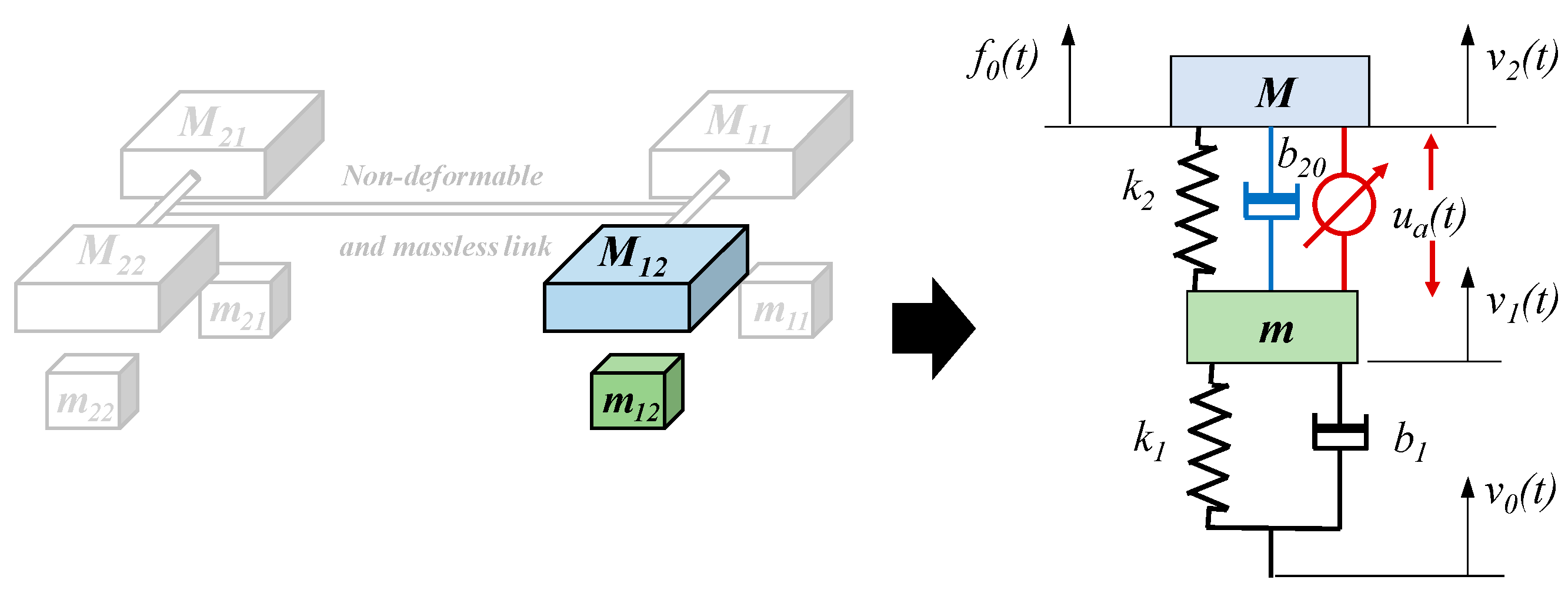
2.1. Quarter-Vehicle Model

Obtaining a 16-DOF simulator is achieved by breaking down the vehicle into five non-deformable solids (the body and the four wheels) (refer to Figure 5a) and then introducing the degrees of connection between these five solids. Furthermore, to attain the vertical load F_zij(t) necessary to describe the behavior of the tire (the Pacejka model, for example) for each wheel, the body assumed to be non-deformable and of mass M_s (sprung mass) is decomposed into four sprung masses M_ij connected to each other by a non-deformable and massless connection (refer to Figure 5b).

Finally, since the proprioceptive sensors intended for suspension control (accelerometers and travel sensors) are located at the four corners of the vehicle [33], a quarter-vehicle model with two DOF was chosen for the study presented in this paper (Figure 6). Notably, to make writing easier, the indices i (one for the front and two for the rear) and j (one for the left and two for the right) were deliberately omitted in the case of the quarter vehicle model.

The notations associated with this two-DOF quarter-vehicle model are:

-

m: unsprung mass [kg];

-

M: sprung mass [kg];

-

k₁: vertical stiffness [N/m] of the tire;

-

k₂: stiffness [N/m] of the suspension spring;

-

b₁: equivalent viscous friction coefficient [Ns/m] of the tire;

-

b₂₀: equivalent viscous friction coefficient [Ns/m] of the active suspension shock absorber;

-

v₀(t): vertical speed [m/s] of the tire contact point on the road (road input);

-

v₁(t): vertical speed [m/s] of the unsprung mass m₁;

-

v₂(t): vertical speed [m/s] of the sprung mass m₂;

-

f₀(t): load transfer [N] resulting from the driver’s action on the steering wheel or pedals (brake and accelerator).

For this study, the nominal numerical values of the parameters correspond to those of a right front quarter of a DS7 Crossback [31], i.e.,:

$$\left\{\begin{array}{l}m = 61 \mathrm{kg}\hfill \\ k_1 = \mathrm{250,000} \mathrm{N}/\mathrm{m}\hfill \\ b_1 = 50 \mathrm{Ns}/\mathrm{m}\hfill \end{array}\right.,\left\{\begin{array}{l}M =427 \mathrm{kg}\hfill \\ k_2 = \mathrm{26,760} \mathrm{N}/\mathrm{m}\\ b_{20} = 1040 \mathrm{Ns}/\mathrm{m}\end{array}\right..$$

Note that m << M (M/m = 7), k₂ << k₁ (k₁/k₂ = 9.34), and b₁ << b₂₀ (b₂₀/b₁ = 20.8), characteristic results of passenger vehicles with a natural undamped pulsation of the unsprung mass ${\omega }_{n_1}\approx \sqrt{{\displaystyle \raisebox{1ex}{$k_1$}\!\left/ \!\raisebox{-1ex}{$m$}\right.}}=64 \mathrm{rad}/\mathrm{s} \left(10.2 \mathrm{Hz}\right)$ and a natural undamped pulsation of the sprung mass ${\omega }_{n_2}\approx \sqrt{{\displaystyle \raisebox{1ex}{$k_2$}\!\left/ \!\raisebox{-1ex}{$M$}\right.}}=7.92 \mathrm{rad}/\mathrm{s} \left(1.26 \mathrm{Hz}\right)$, i.e., ω_n1/ω_n2 = 8.1.

All differential equations that describe the dynamic behaviors of unsprung and sprung masses around the static equilibrium position are presented in references [31,34].

Remark 1.

In fault mode (u_a(t) = 0), the damping of the unsprung and sprung masses is ensured only by the dissipative element with the viscous friction coefficient noted as b₂₀ (see Figure 6). The value of b₂₀ is calculated so that in the event of a failure of the active suspension actuator, the vehicle can continue to drive safely until repaired, provided that it remains within ODD1. This fault mode is defined based on the expertise acquired during work with PSA concerning the Citroën Hydractive suspension, particularly in comfort mode (suspension in soft mode), where the wheel damping factor ζ₁ = b₂₀/(2 (m (k₁ + k₂))) is only 0.13, while this same factor is 0.35 in road handling mode (suspension in hard mode) [28].

2.2. Measurement Noise Model

The noise model associated with the measurement of the acceleration a₁(t) of the unsprung mass is the “Uniform Random Number” model of Simulink, centered around zero with the limits B_1min = −0.3145 m/s² and B_1max = 0.3145 m/s². These numerical values were obtained following an experimental campaign aimed at determining the metrological characteristics of the sensor [33].

Figure 7 shows the evolution of the measurement noise n₁(t) (in m/s²) from such a model.

2.3. Random Road Profiles

The International Organization for Standardization provides a method for describing and classifying road profiles based on the power spectral density (PSD) of the vertical displacement z₀(t) of the road profile; this is the ISO 8608 standard [35]. This standard proposes a classification of road profiles from class A (motorway in very good condition) to class E (secondary road in very poor condition). From this data, it is possible to generate random road profiles with different geometric characteristics while belonging to a desired road profile class. Among the different existing methods to generate a random road profile [36], the method chosen in this article is the shaping filter method, with a band-limited white noise as input. In [36], full details for the generation of the ISO Class B road profile used in this paper are provided.

Figure 8 shows the evolution of the road profile z₀(t) (in cm) from the “Random Road Profile” model for an ISO Class B road and for a longitudinal translation speed V_x = 30 m/s (108 km/h).

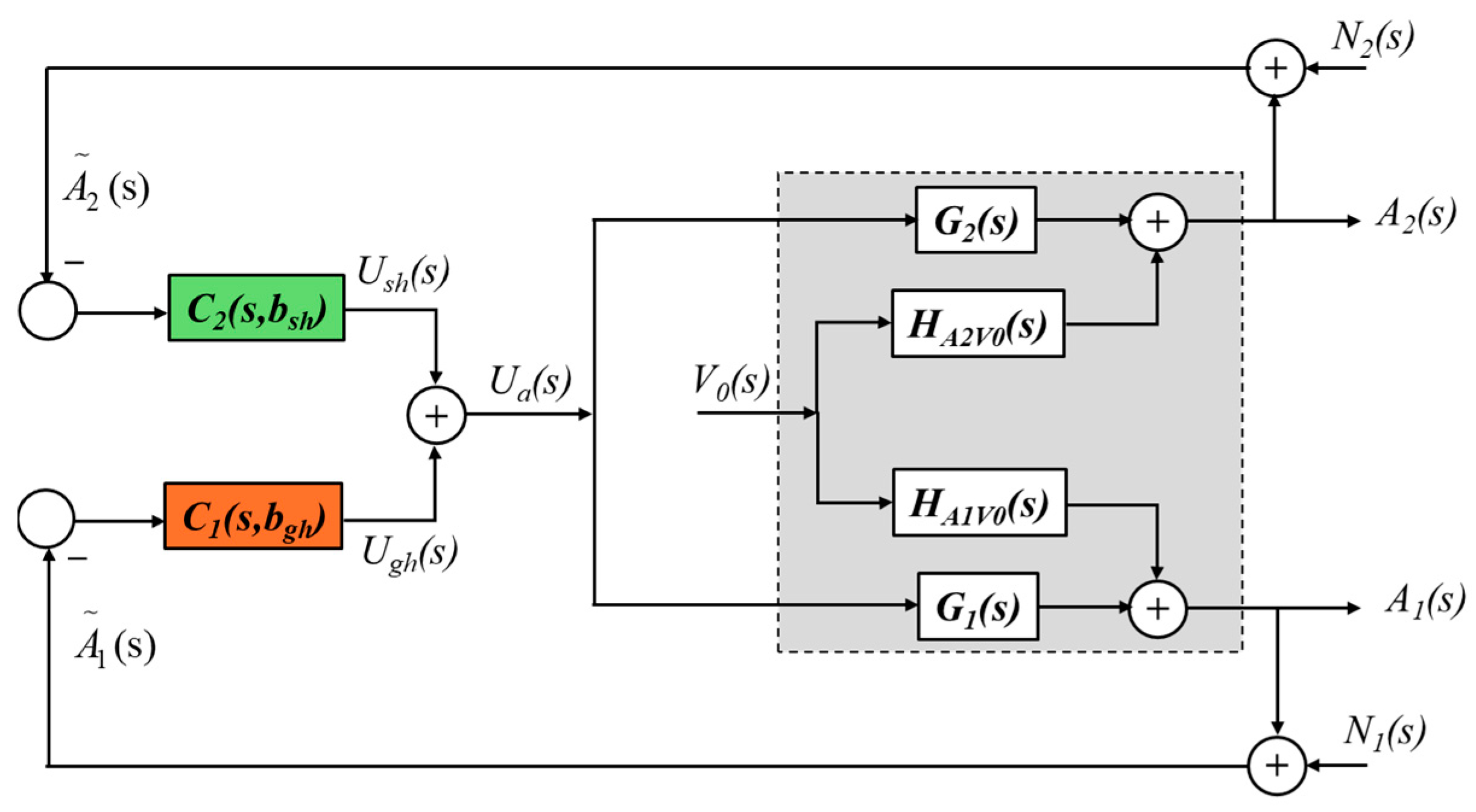
3. Suspension Control Architecture

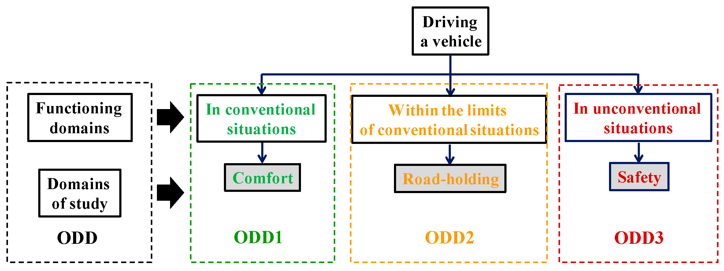
3.1. General Case Regardless of the ODD

Suspension control is part of a broader framework of vehicle-wide hierarchical control and overall chassis control [9,10]. In this context, the supervisor plays a key role in receiving information not only from the vehicle’s proprioceptive and exteroceptive sensors but also from the infrastructure (V2X) and other vehicles (V2V). In the case of suspension control (Figure 9), the supervisor is able to estimate the operating domain (ODD1, ODD2, or ODD3) in which the vehicle is located and to choose the corresponding strategy (refer to Figure 4).

Figure 10 shows the functional diagram of the suspension control architecture regardless of the ODD; this is in the absence of load transfer F₀(s) $\left(F_0\left(s\right)=\mathrm{LT}\left\{f_0\left(t\right)\right\}=0\right)$.

$V_0\left(s\right)$ represents the disturbance from the road profile $\left(V_0\left(s\right)=\mathrm{LT}\left\{v_0\left(t\right)\right\}\right)$, N_i(s) (i = 1 and 2) represents the measurement noise $\left(N_i\left(s\right)=\mathrm{LT}\left\{n_i\left(t\right)\right\}\right)$ of the acceleration A_i(s), and $\left(A_i\left(s\right)=\mathrm{LT}\left\{a_i\left(t\right)\right\}\right)$, ${\tilde{A}}_i\left(s\right)=A_i\left(s\right)+N_i\left(s\right)$ represents the measure of acceleration $A_i\left(s\right)$ $\left({\tilde{A}}_i\left(s\right)=\mathrm{LT}\left\{{\tilde{a}}_i\left(t\right)\right\}\right)$. Finally, the force command $U_a\left(s\right)=\mathrm{LT}\left\{u_a\left(t\right)\right\}$ results from the GH U_gh(s) command and the SH U_sh(s) command. Indeed (Figure 4), for ODD1, U_a(s) = U_sh(s), because U_gh(s) = 0; for ODD2, U_a(s) = U_gh(s) + U_sh(s); for ODD3, U_a(s) = U_gh(s), because U_sh(s) = 0.

Furthermore, the different transfer functions that appear in this functional diagram are defined by (see references [31,34] for more details):

$${\left.G_1\left(s\right)={\displaystyle \frac{A_1\left(s\right)}{U_a\left(s\right)}}\right|}_{\begin{array}{l}{F}_0=0\\ V_0=0\end{array}} = -{\displaystyle \frac{M s^4}{Den\left(s\right)}},$$

(1)

$${\left.G_2\left(s\right)={\displaystyle \frac{A_2\left(s\right)}{U_{sh}\left(s\right)}}\right|}_{\begin{array}{l}{V}_0=0\\ F_0=0\end{array}} = {\displaystyle \frac{s^2\left(m s^2+b_1 s+k_1\right)}{Den\left(s\right)}},$$

(2)

$${\left.H_{A_1{V}_0}\left(s\right)={\displaystyle \frac{A_1\left(s\right)}{V_0\left(s\right)}}\right|}_{\begin{array}{l}{U}_a=0\\ F_0=0\end{array}} = {\displaystyle \frac{s \left(b_1 s+k_1\right)\left(M s^2+b_{20} s+k_2\right)}{Den\left(s\right)}}$$

(3)

and

$${\left.H_{A_2{V}_0}\left(s\right)={\displaystyle \frac{A_2\left(s\right)}{V_0\left(s\right)}}\right|}_{\begin{array}{l}{U}_a=0\\ F_0=0\end{array}} = {\displaystyle \frac{s \left(b_1 s+k_1\right)\left(b_{20} s+k_2\right)}{Den\left(s\right)}},$$

(4)

with

$$\begin{array}{l}Den\left(s\right)=M m s^4+\left(\left(M+m\right)b_{20}+M b_1\right) s^3+\left(M\left(k_1+k_2\right)+m k_2+b_1 b_{20}\right) s^2\\ \hspace{1em}\hspace{1em}\hspace{1em}\hspace{1em}+\left(k_1 b_{20}+k_2 b_1\right) s+k_1 k_2\end{array}$$

(5)

Finally, the transfer function of the SH regulator, noted as C₂(s), is defined in [30], and that of the GH regulator, noted as C₁(s), is defined in the following paragraph.

3.2. Special Case: ODD3 and CGH

As a reminder, at the functional level, the classic GH strategy is defined by a force feedback law in the form u_gh(t) = −b_gh v₁(t), where u_gh(t) denotes the force developed by the suspension actuator, v₁(t) the vertical speed of the unsprung mass, and b_gh the GH gain (negative constant).

From a control theory point of view, the functional diagram associated with the GH strategy clearly highlights the presence of a speed regulation loop v₁(t) of the unsprung mass m (wheel) around zero. In this diagram, the transfer function C_v1(s) of the controller is reduced to a proportional action of gain b_gh, i.e., C_v1(s) = b_gh. This control law can be classified into the category of partial state feedback controls.

In practice, since the vertical speed v₁(t) of the unsprung mass m is not measured, two solutions are possible for implementing the GH strategy. The first consists of using a model-based state observer powered, in particular, by measurements from the proprioceptive sensors of the suspension, thus making it possible to obtain an estimate of the vertical speed ${\widehat{v}}_1\left(t\right)$. The second is to directly use the available measurement of the acceleration a₁(t) of the unsprung mass. In this case, the associated functional diagram highlights that the implementation of the GH strategy from the measurement of the vertical acceleration a₁(t) consists of regulating a₁(t) around zero. The transfer function C₁(s) of the controller (Figure 8) then comes down to an integral action with a constant b_gh, i.e., C₁(s) = b_gh/s.

The regulation of v₁(t) or a₁(t) around zero is, in fact, only an intermediate objective, because the main objective of the GH strategy is to minimize the vertical variation f_z(t) of the load F_z(t) on the wheel defined by:

$$F_z\left(t\right)=F_z^e+f_z\left(t\right),$$

(6)

where $F_z^e$ represents the static load on each wheel (vehicle weight distributed over the four wheels; here, $F_z^e=\left(M+m\right)g$) and f_z(t) represents the variation around $F_z^e$. f_z(t) depends, in particular, on the variations v₀(t) of the road profile, as well as the load transfers f₀(t) when cornering and during acceleration/braking phases. This component, F_z(t), makes the link between the vertical dynamics and the horizontal dynamics of the vehicle through the tire. Indeed, the longitudinal $F_x\left(t\right)=F_x^e+f_x\left(t\right)$ and transverse forces $F_y\left(t\right)=F_y^e+f_y\left(t\right)$ of the tire/ground interface are a function, in particular, but not only, of F_z(t). In ODDs 2 and 3, the f_z(t) variations are significant enough to cause significant f_x(t) and f_y(t) variations, which disrupt the dynamic balance of the vehicle and therefore its road-holding. It is therefore essential to minimize the variations f_z(t). Notably, this is not the case in ODD1.

Furthermore, in order to study the performance of the control loop resulting from such a configuration, the functional equations of the output A₁(s) and of the control U_a(s) are established from the functional diagram in Figure 8 in the case where U_sh(s) = 0 (ODD3), i.e.,:

-

for the output A₁(s):

$$A_1\left(s\right)=\left[S_1\left(s\right) H_{A_1{V}_0}\left(s\right)\right] V_0\left(s\right)-\left[T_1\left(s\right)\right] N_1\left(s\right);$$

(7)

-

for the control U_a(s):

$$U_a\left(s\right)=-\left[R_1\left(s\right)H_{A_1{V}_0}\left(s\right)\right] V_0\left(s\right)-\left[R_1\left(s\right)\right] N_1\left(s\right),$$

(8)

where the sensitivity functions S₁, T₁, and R₁ are given by:

$$S_1\left(s\right) ={\displaystyle \frac{1}{1+{\beta }_1\left(s\right)}},T_1\left(s\right)=1-S_1\left(s\right),R_1\left(s\right) =C_1\left(s\right)S_1\left(s\right),$$

(9)

and where β₁(s) represents the open-loop transfer function defined by:

$${\beta }_1\left(s\right) =C_1\left(s\right) G_1\left(s\right).$$

(10)

Thus, according to Equation (7), the function S₁ makes it possible to analyze, in the frequency domain, the influence of the control loop on the sensitivity of the output A₁(s) to the disturbance V₀(s). Indeed, in fault mode (no regulation, U_a(s) = 0), the function S₁ = 1, and the sensitivity of A₁(s) to V₀(s) is directly linked to H_A1V0(s).

Similarly, according to Equation (8), the function T₁ allows us to analyze, in the frequency domain, the sensitivity of the output A₁(s) to the measurement noise N₁(s). In fault mode (U_a(s) = 0), the function T₁ = 0, thus reflecting an insensitivity of the output A₁(s) to measurement noise over the entire frequency space.

Finally, the R₁ function allows us to analyze, in the frequency domain, the sensitivity of the U_a(s) command to the measurement noise N₁(s) and to the disturbance V₀(s) (Equation (9)). In fault mode, the R₁ function = 0.

In this context, the controller associated with the generalized crone ground hook (CGHG) strategy is defined by:

$$C_1\left(s\right) = {\displaystyle \frac{b_{gh}}{s^{{\nu }_1}}},$$

(11)

with b_gh < 0 et ${\nu }_1 \in \left[0 ; 2\right]$.

The generalized crone ground hook (CGHG) strategy is defined by two parameters (relation (11)), namely the constant b_gh and the fractional integration order ν₁ between 0 and 2. This strategy is part of the theory of fractional systems, which allows us, with a small number of parameters (here, two parameters: b_gh and ν₁), to cover a wide range of behaviors.

So, from a behavioral point of view:

-

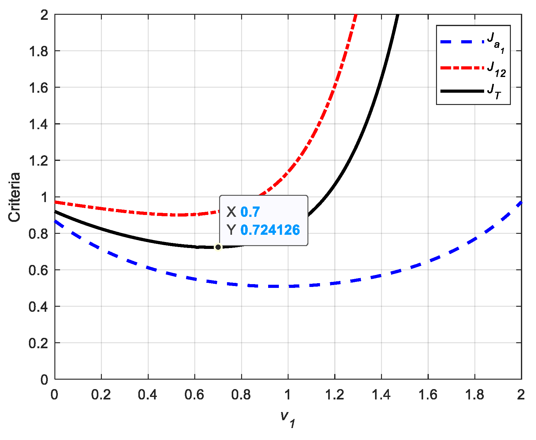
ν₁ = 0 => inertial behavior [37];

-

0 < ν₁ < 1 => visco-inertial behavior;

-

ν₁ = 1 => viscous behavior;

-

1 < ν₁ < 2 => viscoelastic behavior;

-

ν₁ = 2 => elastic behavior.

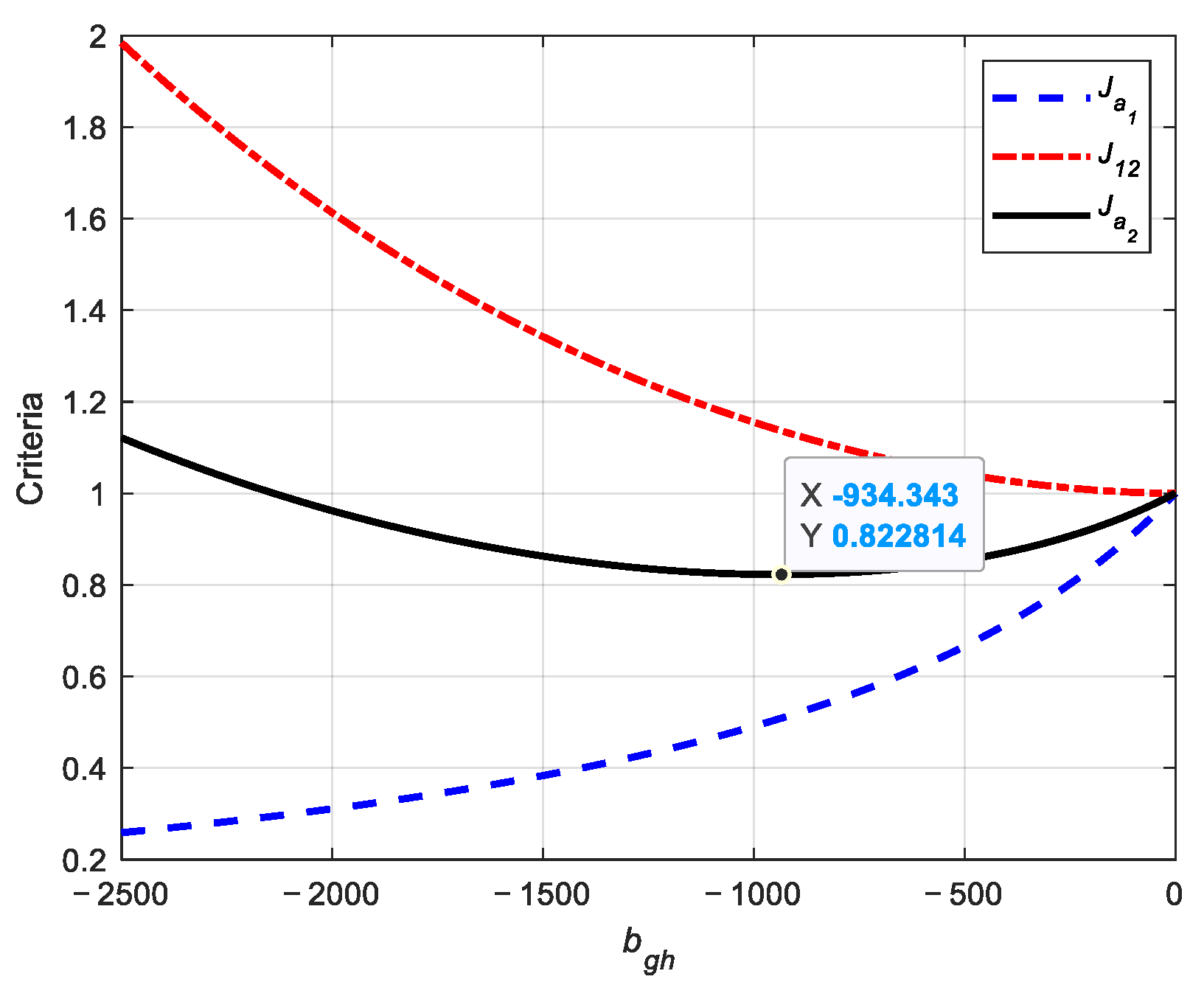
3.3. Optimal Parameters of the CGH Strategy

Due to the existence of an acceleration-suspension travel dilemma [28], the two variables considered for the definition of the criteria used for optimization in the ODD3 are:

-

the acceleration a₁(t) of the unsprung mass;

-

the suspension travel z₁₂(t) = z₁(t) − z₂(t), where z_i(t) represents the vertical displacement of the unsprung mass (i = 1) and the sprung mass (i =2).

Taking into account the road profile generating process (Section 2.2), the two criteria $J_{a_1}$ and $J_{z_{12}}$ [28] are defined by:

$$J_{a_1}\left(b_{gh},{\nu }_1\right)= {\displaystyle \frac{ {\displaystyle \underset{{\omega }_{\mathit{min}}}{\overset{{\omega }_{\mathit{max}}}{\int }}{\left|H_{a_1}\left(j\omega ,b_{gh},{\nu }_1\right)\right|}^{2}d\omega }}{ {\displaystyle \underset{{\omega }_{\mathit{min}}}{\overset{{\omega }_{\mathit{max}}}{\int }}{\left|H_{a_1}\left(j\omega ,0,0\right)\right|}^{2}d\omega }}}$$

(12)

and

$$J_{z_{12}}\left(b_{gh},{\nu }_1\right)= {\displaystyle \frac{ {\displaystyle \underset{{\omega }_{\mathit{min}}}{\overset{{\omega }_{\mathit{max}}}{\int }}{\left|H_{z_{12}}\left(j\omega ,b_{gh},{\nu }_1\right)\right|}^{2}d\omega }}{ {\displaystyle \underset{{\omega }_{\mathit{min}}}{\overset{{\omega }_{\mathit{max}}}{\int }}{\left|H_{z_{12}}\left(j\omega ,0,0\right)\right|}^{2}d\omega }}},$$

(13)

with ω_min = 2π 0.1 rad/s and ω_max = 2π 30 rad/s, and where each term in the denominator corresponds to the value of the criterion in fault mode (U_a(s) = 0). Thus, the interpretation of the results is facilitated, as any value of $J_{a_1}$ and $J_{z_{12}}$ less than unity reflects an improvement compared to the fault mode and, conversely, any value greater than unity reflects a deterioration compared to the fault mode.

The process of finding the optimal parameters b_gh and ₁ is carried out in two steps.

The first step is to set ν₁ = 1, thus defining the crone ground hook nominal (CGHN) strategy.

For the example treated, Figure 11 presents, as a function of the gain b_gh, the variations of criteria $J_{a_1}$ (in blue) and $J_{z_{12}}$ (in red), as well as the variation of the global criterion J_T (in black) defined by:

$$J_T\left(b_{gh},1\right)= {\displaystyle \frac{J_{a_1}\left(b_{gh},1\right)+J_{z_{12}}\left(b_{gh},1\right)}{2}}.$$

(14)

Compared to the fault mode (horizontal line for criteria = 1, Figure 11), the observation in Figure 11 highlights that an increase in the absolute value of b_gh, i.e., $\left|b_{gh}\right|$, leads to a decrease in $J_{a_1}$ and an increase in $J_{z_{12}}$, thus reflecting the presence of a dilemma, which justifies the use of the global criterion J_T. Thus, the minimum value of J_T (min[J_T] = 0.823, corresponding to a 17.7% improvement compared to the fault mode) is obtained for b_gh = −934 Ns/m.

The second step consists of determining ν₁ and b_gh with an iso-rapidity constraint fixed by ω_−3dB. ω_−3dB represents the upper frequency limit of the −3dB bandwidth of the CGHN control loop. Thus, the value pair (b_gh; ν₁) is determined with a constraint ensuring an identical dynamics speed of the CGHG loop with respect to the CGHN loop.

Figure 12 shows, as a function of order ν₁, the variations of criteria $J_{a_1}$ (in blue) and $J_{z_{12}}$ (in red), as well as the variation of the global criterion J_T (in black). The minimum value of J_T (min[J_T] = 0.724, corresponding to a 27.6% improvement compared to the fault mode) is obtained for ν₁ = 0.7 and b_gh = −252 Ns^0.7/m.

4. Performance

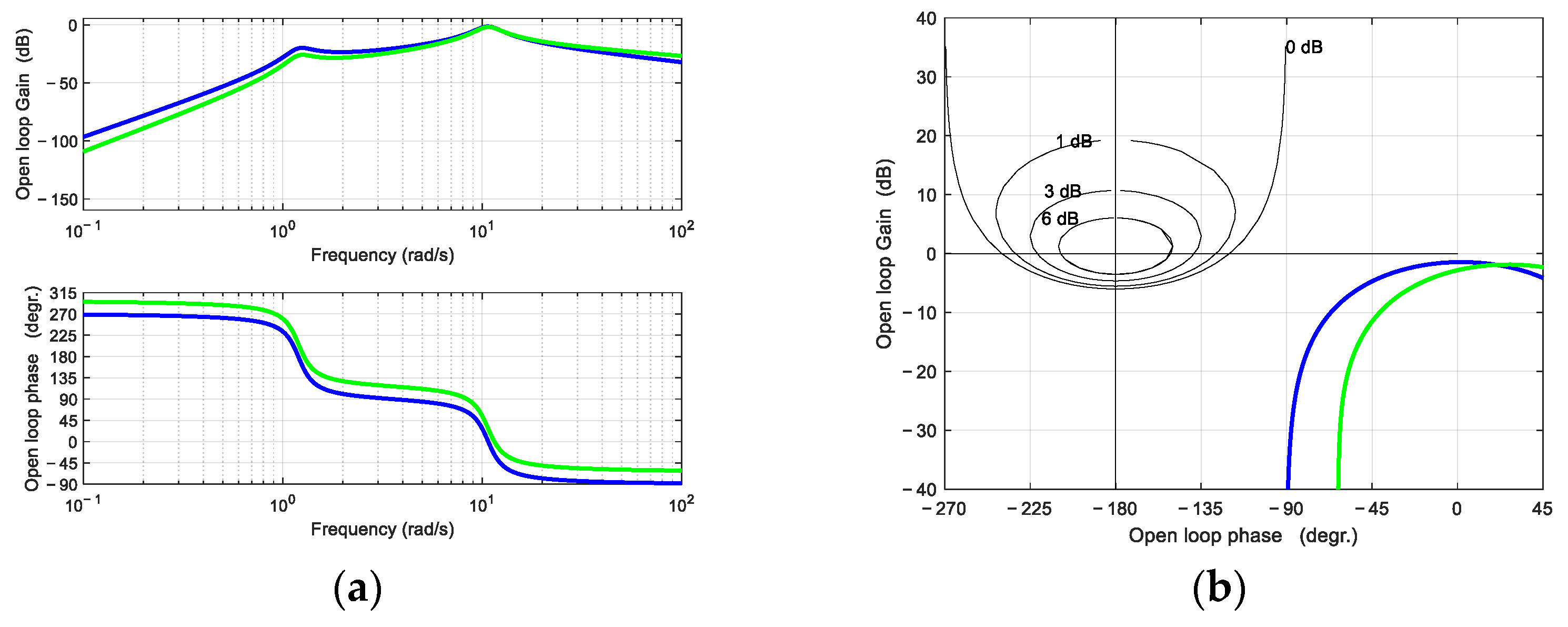
4.1. Performance from a Control Theory Perspective

From a control theory point of view, the responses selected for the analysis are:

-

in the frequency domain:

-

the Bode plots of the frequency response β₁(jω), as well as its Black-Nichols loci;

-

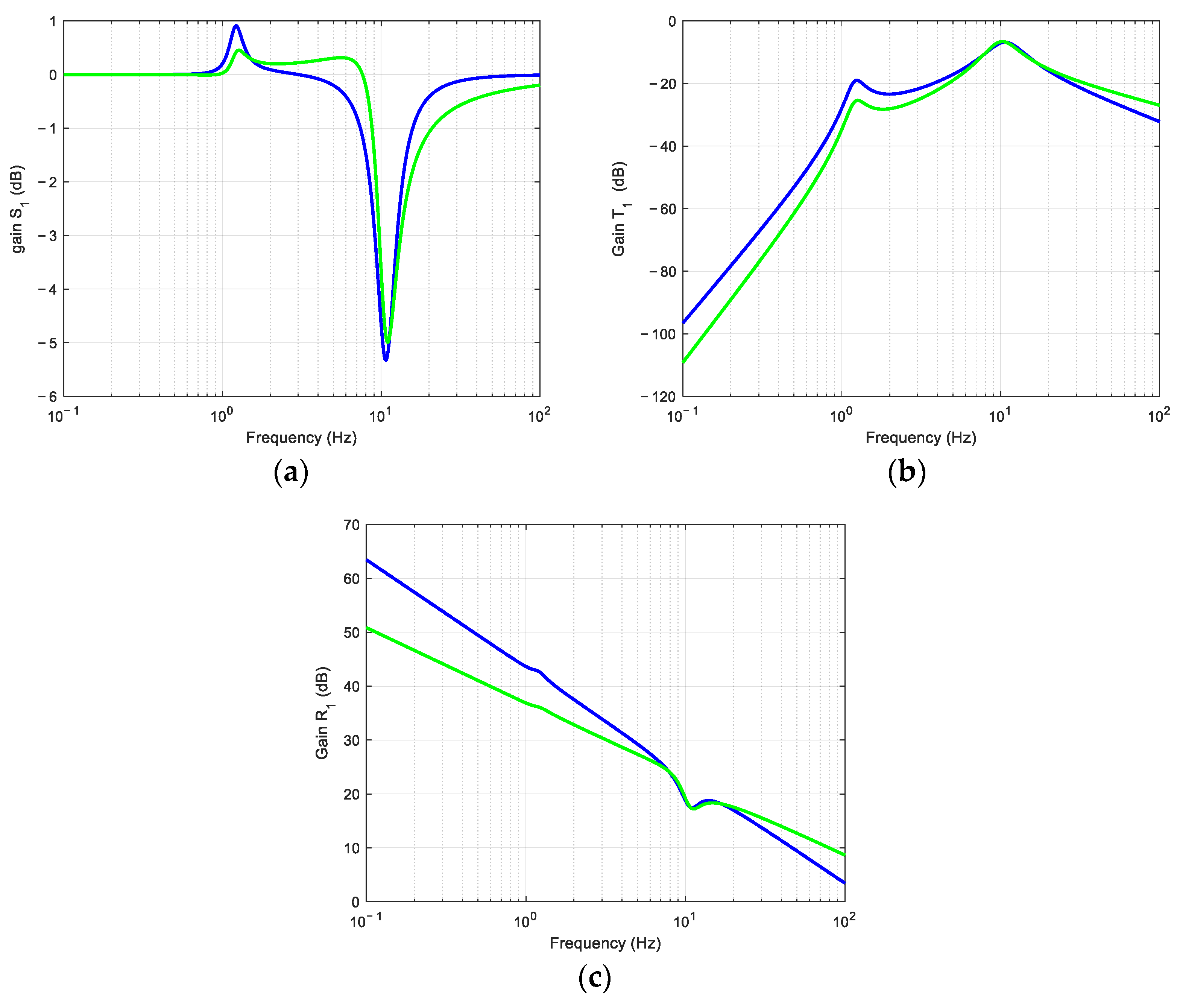
the gain diagrams of the sensitivity functions S₁, T₁, and R₁;

-

in the time domain:

-

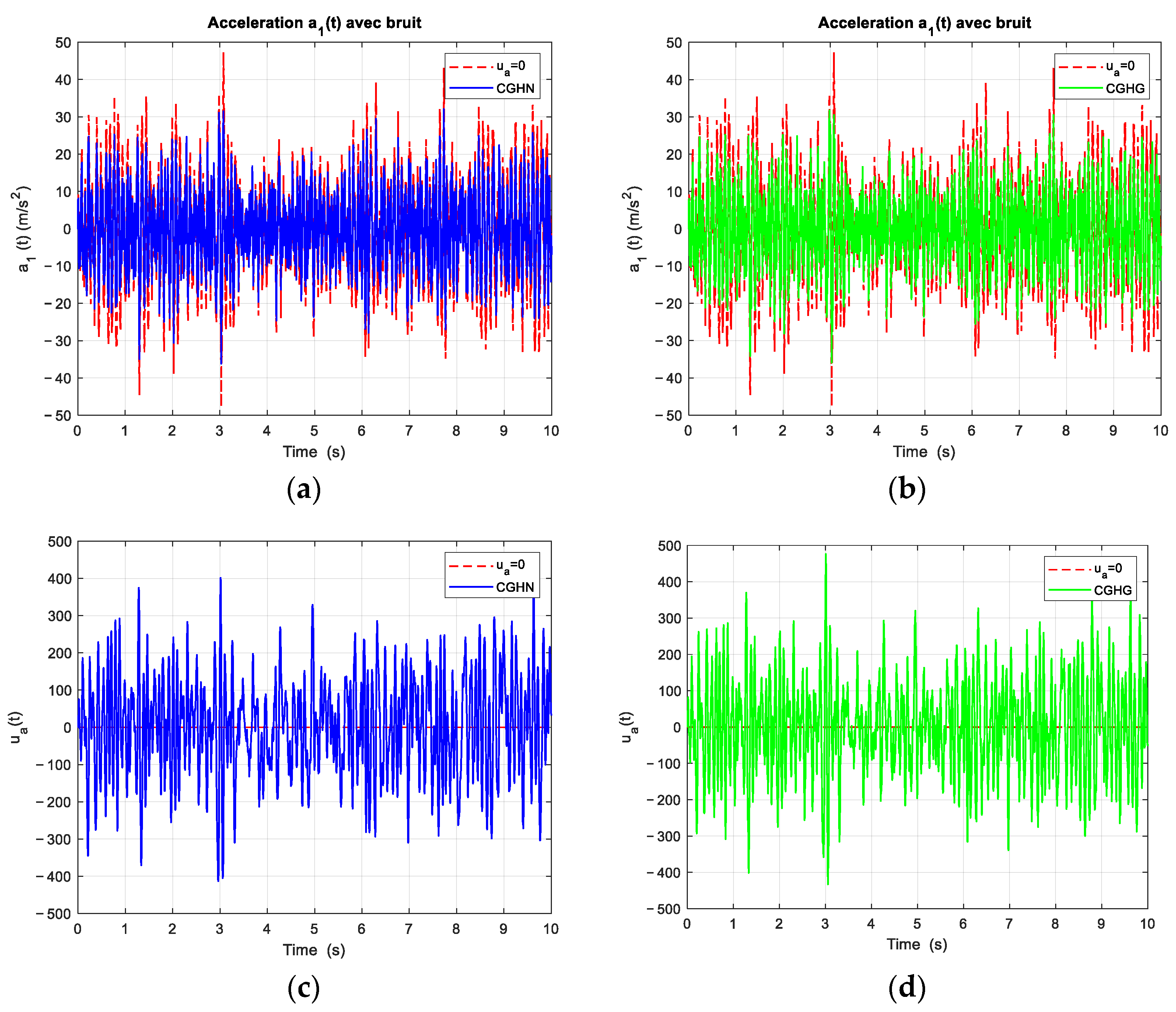
the vertical acceleration a₁(t) as a regulated quantity;

-

the force control u_a(t) (verification of the risk of saturation and of the sensitivity to measurement noise).

Figure 13 shows the Bode plots (a) and Black-Nichols loci (b) of the open-loop transfer function β₁(s) obtained with the CGHN (blue) and CGHG (green) strategies.

Figure 14 shows the gain diagrams of the sensitivity functions S₁ (a), T₁ (b), and R₁ (c) obtained with the CGHN (in blue) and CGHG (in green) strategies.

Compared to the fault mode (no regulation, U_a(s) = 0), where the function S₁ = 1 (0 dB), the regulation loop leads to (refer to Figure 14a):

-

a local increase in the vicinity of the natural pulsation ω_n2 of the sprung mass,

-

a local decrease in the vicinity of the natural pulsation ω_n1 of the unsprung mass of the sensitivity of output A₁(s) to disturbance V₀(s).

Similarly, compared to the fault mode, where the function T₁ = 0 in linear scale, the control loop leads to a maximum sensitivity of 0.46 in linear scale (−6.7 dB) of the output A₁(s) to the measurement noise N₁(s) in the vicinity of the natural pulsation ω_n1 (Figure 14b).

Finally, still compared to the fault mode, where the function R₁ = 0 on a linear scale, the control loop inexorably leads to an increase in the sensitivity of the U_a(s) command to the measurement noise N₁(s) and to the disturbance V₀(s).

Remark 2.

From a general point of view, in control theory, it is necessary to limit the gain of the controller in high frequencies to limit the sensitivity of the control signal to measurement noise. This sensitivity is quantified using the sensitivity function R₁, defined by relation (8).

In the particular case of the sky hook (SH) and ground hook (GH) approaches implemented from the measurement of the acceleration (of the sprung mass for SH or of the unsprung mass for GH), the expression of the controller is that of an integrator (relation (11)).

This is the reason why the gain of the sensitivity function R1 tends towards zero as the frequency tends towards infinity (see Figure 14c), thus minimizing the sensitivity of the control signal to measurement noise. There is therefore no need to add any specific constraint when designing the controller with regard to measurement noise.

Figure 15 shows the time responses a₁(t) ((a) and (b)) and u_a(t) ((c) and (d)) obtained with the CGHN (in blue) and CGHG (in green) strategies, as well as with the fault mode (in red), and when the road profile applied is that of an ISO Class B road with V_x = 30 m/s (108 km/h).

These time responses confirm:

-

a decrease in the sensitivity of the vertical acceleration a₁(t) to the perturbation v₀(t) of the road profile compared to the failing mode (in red), and for both strategies CGHN and CGHG (refer to Figure 15a,b);

-

the absence of saturation of the u_a(t) command (Figure 15c,d).

4.2. Performance from a Vibration Study Point of View

In the frequency domain, the performance is analyzed qualitatively using the gain diagrams (plotted in lin-lin scale: linear scale for gain and frequency) of the transfers:

-

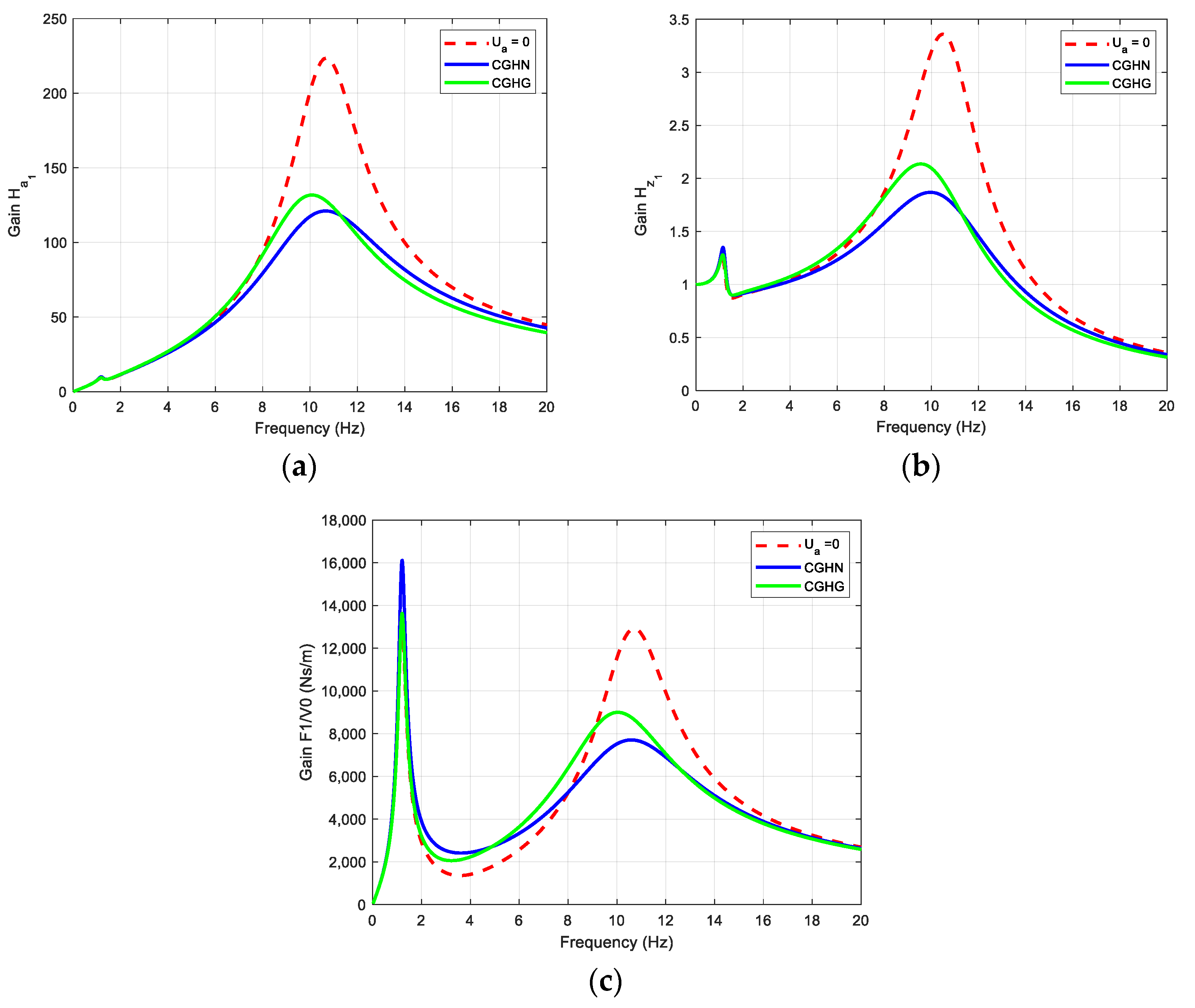
for comfort: $H_{a_2}\left(s\right)$ = A₂(s)/V₀(s) on the interval [0; 20] Hz; $H_{z_2}\left(s\right)$ = Z₂(s)/Z₀(s) = V₂(s)/V₀(s) on the interval [0; 5.5] Hz;

-

for operation: $H_{z_{12}}\left(s\right)$ = Z₁₂(s)/V₀(s) on the interval [0; 20] Hz;

-

for wheel holding: $H_{a_1}\left(s\right)$ = A₁(s)/V₀(s), $H_{z_1}\left(s\right)$ = Z₁(s)/Z₀(s) = V₁(s)/V₀(s), and $H_{f_z}\left(s\right)$ = F_z(s)/V₀(s) on the interval [0; 20] Hz.

Still, in the frequency domain, performances are analyzed quantitatively using performance indices of the form:

$$J_x\left(b_{gh},{\nu }_1\right)= {\displaystyle \frac{ {\displaystyle \underset{{\omega }_{\mathit{min}}}{\overset{{\omega }_{\mathit{max}}}{\int }}{\left|H_x\left(j\omega ,b_{gh},{\nu }_1\right)\right|}^{2}d\omega }}{ {\displaystyle \underset{{\omega }_{\mathit{min}}}{\overset{{\omega }_{\mathit{max}}}{\int }}{\left|H_x\left(j\omega ,0,0\right)\right|}^{2}d\omega }}},$$

(15)

with

-

b_gh = −934 Ns/m and ν₁ = 1, for the CGHN strategy (see Figure 11);

-

b_gh = −252 Ns^0.7/m and ν₁ = 0.7, for the CGHG strategy (see Figure 12),

-

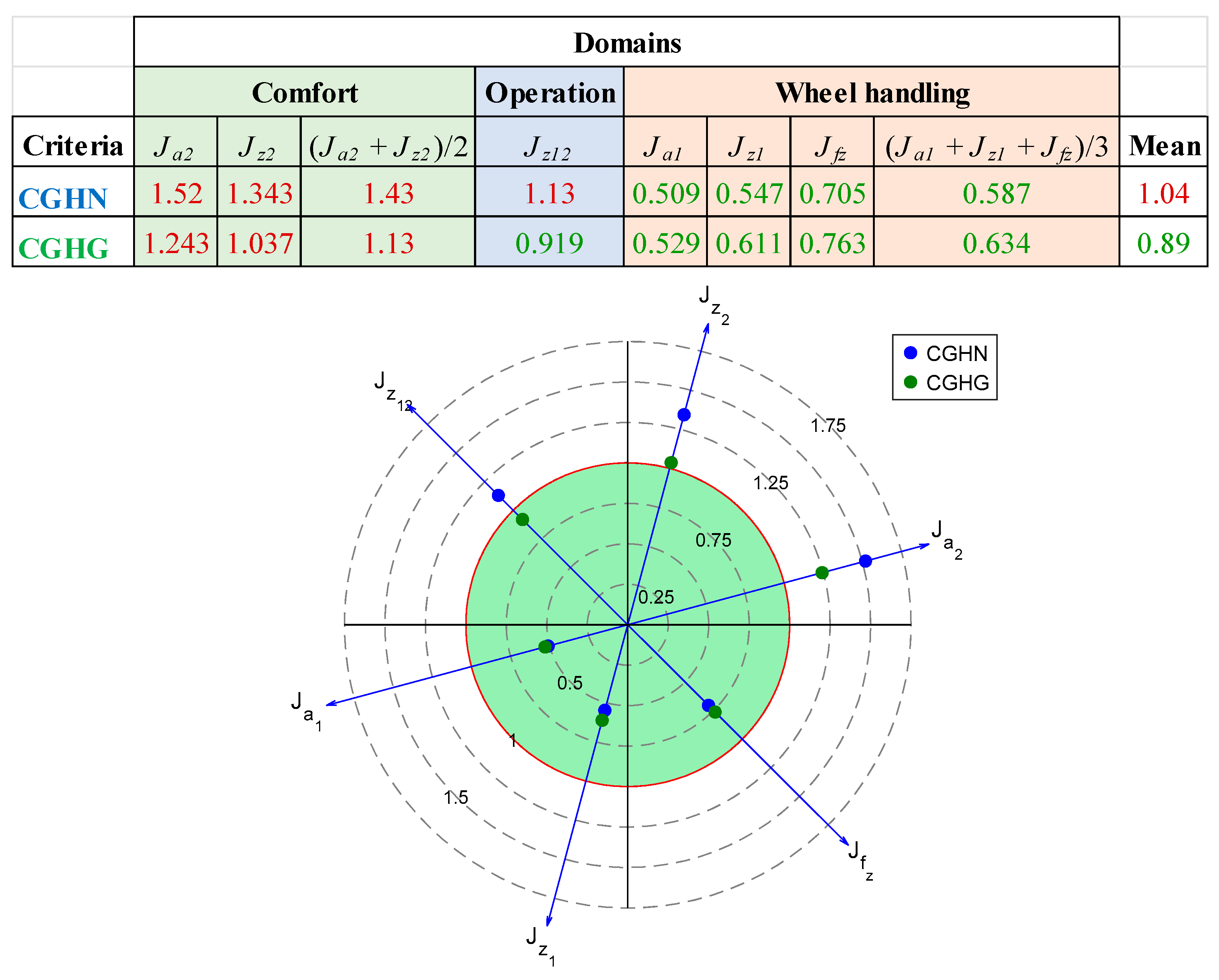
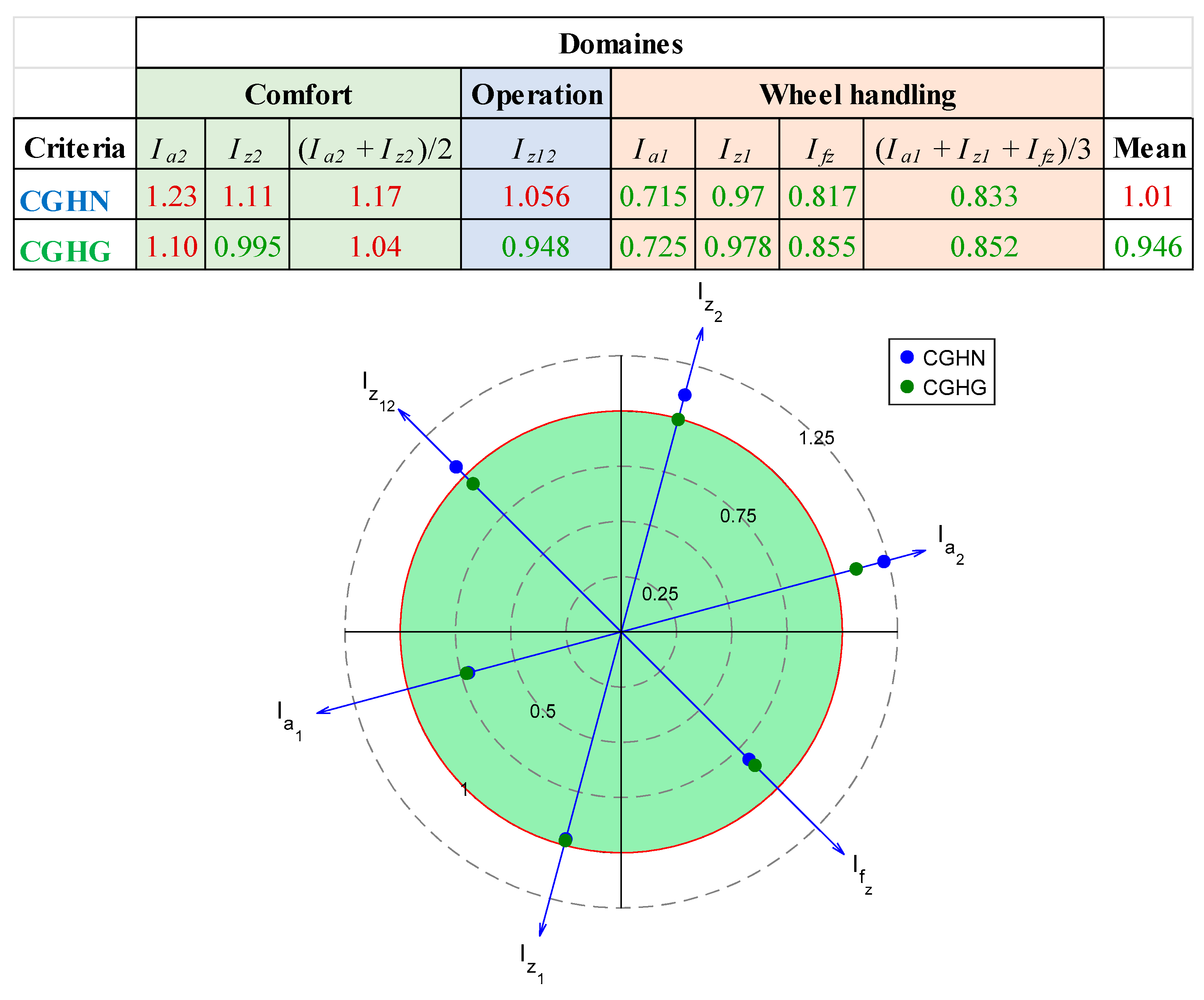
and where, according to the criteria, the variable x represents:

-

for comfort, the vertical acceleration a₂ and the vertical displacement z₂ of the sprung mass M (body);

-

for operation, suspension travel z₁₂ (limited by stroke);

-

for wheel holding, the vertical acceleration a₁ and the vertical displacement z₁ of the unsprung mass m (wheel), as well as the dynamic component f_z of the load on the tire.

Figure 16 shows the gain diagrams of transfers $H_{a_2}\left(s\right)$ (a) and $H_{z_2}\left(s\right)$ (b) obtained with the CGHN (in blue) and CGHG (in green) strategies, as well as with the fault mode (in red).

Figure 17 shows the gain diagrams of transfers $H_{z_{12}}\left(s\right)$ obtained with the CGHN (in blue) and CGHG (in green) strategies, as well as in default mode (in red).

Figure 18 shows the gain diagrams of the transfers $H_{a_1}\left(s\right)$ (a), $H_{z_1}\left(s\right)$ (b), and $H_{f_z}\left(s\right)$ (c) obtained with the CGHN (in blue) and CGHG (in green) strategies, as well as with fault mode (in red).

Figure 19 presents a table summarizing the values of the criteria J_x(b_gh; ν₁) for the two strategies CGHN and CGHG in the areas of comfort, operation, and wheel handling. In this table, all values above unity (degradation) are red, and all values below unity (improvement) are green. The numerical values that appear in the Mean column are equal to the sum of the values of the six J_x components divided by 6. To facilitate analysis, this table is accompanied by a radar plot.

Overall, and compared to the fault mode (u_a = 0), the analysis of the numerical values of the criteria defined in the frequency domain (Figure 19) highlights a known result for the GH strategies, namely that the two strategies, CGHN and CGHG, improve wheel handling but degrade vibration comfort (comfort-wheel handling dilemma).

Comparing each of the scores (average of the six frequency criteria) obtained for the two strategies allows us to affirm that the CGHG strategy is the one that obtains the best result. Indeed, in more detail, the CGHG strategy is the one that:

-

degrades vibration comfort the least (average value of the comfort criterion equal to 1.13 against 1.43 for the CGHN strategy);

-

undermines the acceleration-travel dilemma, since the decrease in the criterion concerning acceleration a₁ is not accompanied by an increase in the criterion concerning suspension travel z₁₂. In fact, the value of the operating criterion is equal to 0.919, which is not the case with the CGHN strategy where the value of this same criterion is equal to 1.13.

On the other hand, if we only focus on the criterion relating to f_z, then it is the CGHN strategy that leads to the best result in terms of minimizing variations in the vertical load on the tire (see Section 3.2) with a criterion value equal to 0.705.

In the time domain, performance is analyzed quantitatively using performance indices defined by the numerical value of the RMS (root mean square), namely:

$$I_x\left(b_{gh},{\nu }_1\right)={\displaystyle \frac{\mathrm{RMS}\left[x\left(t,b_{gh},{\nu }_1\right)\right]}{\mathrm{RMS}\left[x\left(t,0,0\right)\right]}}$$

(16)

always with

-

b_gh = −934 Ns/m and ν₁ = 1, for the CGHN strategy (see Figure 11);

-

b_gh = −252 Ns^0.7/m and ν₁ = 0.7, for the CGHG strategy (see Figure 12).

and where, according to the criteria, the variable x represents:

-

for comfort, the vertical acceleration a₂ and the vertical displacement z₂ of the sprung mass M (body);

-

for operation, suspension travel z₁₂ (limited by stroke);

-

for wheel holding, the vertical acceleration a₁ and the displacement z₁ of the unsprung mass m (wheel), as well as the dynamic component f_z of the load on the tire.

Figure 20 presents a table summarizing the values of the I_x(b_gh; ν₁) criteria for the two strategies CGHN and CGHG in the areas of comfort, operation, and wheel handling. Similarly, all values above unity (degradation) are red and all values below unity (improvement) are green. The numerical values that appear in the Mean column are equal to the sum of the values of the six I_x components divided by 6. To facilitate analysis, this table is accompanied by a radar plot.

Overall, and compared to the fault mode (u_a = 0), the analysis of the numerical values of the criteria defined in the time domain (Figure 20) confirms the results already observed in the frequency domain. Indeed, both the CGHN and CGHG strategies improve wheel handling but degrade vibration comfort (comfort-wheel handling dilemma).

Comparing each of the scores (average of the six-time criteria) obtained for the two strategies confirms that the CGHG strategy is the one that obtains the best result. Indeed, in more detail, the CGHG strategy is indeed one which:

-

degrades vibration comfort the least (average value of the comfort criterion equal to 1.04 against 1.17 for the CGHN strategy);

-

faults the acceleration-deflection dilemma with a value of the operating criterion equal to 0.948 against 1.056 with the CGHN strategy.

On the other hand, if we only focus on the criterion relating to f_z, then it is the CGHN strategy that leads to the best result in terms of minimizing variations in the vertical load on the tire with a criterion value equal to 0.817 against 0.855 with the CGHN strategy.

5. Conclusions and Perspectives

The work presented in this paper is part of the context of the connected autonomous vehicle (CAV).

The first contribution of the authors in this paper concerns the division of the global operational domain (ODD) into three sub-domains relating to comfort (ODD1), road-holding (ODD2), and safety (ODD3). This division into three sub-domains results from an in-depth analysis of the overall dynamics of the vehicle, in particular using a 16-DOF simulator and different scenarios oriented towards comfort, road-holding, or emergency situations. Thus, based on information from the CAV’s proprioceptive and exteroceptive sensors, but also information from the infrastructure (V2X) and other vehicles (V2V), supervision makes it possible, at any time, to identify the ODD in which the vehicle is located and to propose the most appropriate strategy for suspension control.

The second contribution concerns one of two GH strategies, studied specifically for ODD3 from the measurement of the vertical acceleration of the unsprung mass (wheel). More precisely, the CGHG strategy is a generalization of the classical GH approach based on fractional system theory. The interest of fractional systems is to cover a wide range of behaviors with a small number of parameters (here, two parameters: b_gh and ν₁). The proposed optimal approach leads, in particular, to a value of the order of integration ν₁ equal to 0.7, which corresponds to visco-inertial behavior, where the classical GH approach with ν₁ = 1 leads to viscous behavior.

The conclusion of this comparative study is that the CGHG strategy is the one that obtains the best results, both in the frequency domain and in the time domain. In fact, the CGHG strategy is the one that degrades vibration comfort the least and which overcomes the acceleration-travel dilemma. On the other hand, if we focus only on the criterion relating to f_z, then it is the CGHN strategy that leads to the best result in terms of minimizing variations in the vertical load on the tire.

The medium-term perspective for ODD3 is to make a definitive choice between CGHN and CGHG. To achieve this objective, these two versions of the CGH strategy will be applied to a 16-DOF vehicle model where the vehicle stability will be analyzed using the yaw rate and the drift at the center of gravity, and this for emergency situations (avoidance maneuver, braking in a curve with low grip, etc.).

References

- Benine-Neto, A.; Moreau, X.; Lanusse, P. Robust control for an electro-mechanical anti-lock braking system: The CRONE approach. IFAC-PapersOnLine 2017, 50, 12575–12581. [Google Scholar] [CrossRef]
- Monot, N.; Moreau, X.; Neto, A.B.; Rizzo, A.; Aioun, F. Automated vehicle lateral guidance using multi-PID steering control and look-ahead point reference. Int. J. Veh. Auton. Syst. 2021, 16, 38. [Google Scholar] [CrossRef]
- Attia, R.; Orjuela, R.; Basset, M. Dual-mode Control Allocation for Integrated Chassis Stabilization. IFAC Proc. 2014, 47, 11219–11224. [Google Scholar] [CrossRef]
- Chokor, A. Design of Several Centralized and Decentralized Multilayer Robust Control Architectures for Global Chassis Control. Ph.D. Thesis, Université de Technologie de Compiègne, Compiègne, France, 2019. Available online: https://theses.hal.science/tel-02489343 (accessed on 9 December 2024).
- Chou, H.; D’andréa-Novel, B. Global vehicle control using differential braking torques and active suspension forces. Veh. Syst. Dyn. 2005, 43, 261–284. [Google Scholar] [CrossRef]
- Zhang, H.; Li, X.-S.; Shi, S.-M.; Liu, H.-F.; Rachel, G.; Liu, L. Phase Plane Analysis for Vehicle Handling and Stability. Int. J. Comput. Intell. Syst. 2011, 4, 1179–1186. [Google Scholar] [CrossRef]
- Sun, W.; Tian, J.; Li, S.; Yang, Z.; Ma, Z. Stability Analysis of Vehicle Negotiating a Curve in the Plane. Adv. Mech. Eng. 2013, 5, 893835. [Google Scholar] [CrossRef]
- Bobier-Tiu, C.; Beal, C.; Kegelman, J.; Hindiyeh, R.; Gerdes, J. Vehicle control synthesis using phase portraits of planar dynamics. Veh. Syst. Dyn. 2018, 57, 1318–1337. [Google Scholar] [CrossRef]
- Termous, H. Hierarchical Approach for the Global Chassis Control of an Electric Vehicle. Ph.D. Thesis, Université de Bordeaux, Bordeaux, France, 2020. Available online: https://theses.hal.science/tel-02977884 (accessed on 9 December 2024).
- Termous, H.; Moreau, X.; Francis, C.; Shraim, H. Hierarchical Approach for Driver Disturbance Rejection in an Electric Vehicle: The CRONE Approach. IEEE Trans. Veh. Technol. 2022, 71, 7008–7022. [Google Scholar] [CrossRef]
- Zin, A.; Sename, O.; Gaspar, P.; Dugard, L.; Bokor, J. Robust LPV– ∞ control for active suspensions with performance adaptation in view of global chassis control. Veh. Syst. Dyn. 2008, 46, 889–912. [Google Scholar] [CrossRef]
- Savaresi, S.M.; Poussot-Vassal, C.; Spelta, C.; Sename, O.; Dugard, L. Semi-Active Suspension Control Design for Vehicles; Elsevier: Amsterdam, The Netherlands, 2010. [Google Scholar]
- Androulakis, V. Development of an Autonomous Navigation System for the Shuttle Car in Underground Room & Pillar Coal Mines. Ph.D. Thesis, University of Kentucky, Lexington, KY, USA, 2021. [Google Scholar] [CrossRef]
- Choi, S.B.; Choi, Y.T.; Park, D.W. A sliding mode control of a full-car electrorheological suspension system via hardware in-the-loop simulation. J. Dyn. Syst. Meas. Control 2000, 122, 114–121. [Google Scholar] [CrossRef]
- Tseng, H.E.; Hrovat, D. State of the art survey: Active and semi-active suspension control. Veh. Syst. Dyn. 2015, 53, 1034–1062. [Google Scholar] [CrossRef]
- Hrovat, D. Survey of Advanced Suspension Developments and Related Optimal Control Applications. Automatica 1997, 33, 1781–1817. [Google Scholar] [CrossRef]
- Casciati, F.; Rodellar, J.; Yildirim, U. Active and semi-active control of structures—Theory and applications: A review of recent advances. J. Intell. Mater. Syst. Struct. 2012, 23, 1181–1195. [Google Scholar] [CrossRef]
- Kissai, M.; Monsuez, B.; Tapus, A.; Mouton, X.; Martinez, D. Gain-Scheduled H∞ for Vehicle High-Level Motion Control. In Proceedings of the 6th International Conference on Control, Mechatronics and Automation, in ICCMA 2018, Tokyo, Japan, 12–14 October 2018; Association for Computing Machinery: New York, NY, USA, 2018; pp. 97–104. [Google Scholar]
- Esmailzadeh, E.; Fahimi, F. Optimal Adaptive Active Suspensions for a Full Car Model. Veh. Syst. Dyn. 1997, 27, 89–107. [Google Scholar] [CrossRef]
- Fialho, I.J.; Balas, G.J. Design of Nonlinear Controllers for Active Vehicle Suspensions Using Parameter-Varying Control Synthesis. Veh. Syst. Dyn. 2000, 33, 351–370. [Google Scholar] [CrossRef]
- Cherry, A.S.; Jones, R.P. Fuzzy logic control of an automotive suspension system. IEE Proc.-Control Theory Appl. 1995, 142, 149–160. [Google Scholar] [CrossRef]
- Titli, A.; Boverie, S. Fuzzy and neuro control for semi–active and active suspension. In Advances in Automotive Control 1995; Kiencke, U., Guzzella, L., Eds.; IFAC Postprint Volume; Pergamon: Oxford, UK, 1995; pp. 49–53. [Google Scholar] [CrossRef]
- Emura, J.; Kakizaki, S.; Yamaoka, F.; Nakamura, M. Development of the Semi-Active Suspension System Based on the Sky-Hook Damper Theory. SAE Trans. 1994, 103, 1110–1119. [Google Scholar]
- Poussot-Vassal, C.; Sename, O.; Dugard, L.; Ramirez-Mendoza, R.; Flores, L. Optimal skyhook control for semi-active suspensions. IFAC Proc. 2006, 39, 608–613. [Google Scholar] [CrossRef]
- Hu, Y.; Chen, M.Z.Q. Stability analysis for active control with a sky-hook and ground-hook inerter-damper configuration. In Proceedings of the 2019 IEEE 58th Conference on Decision and Control (CDC), Nice, France, 11–13 December 2019; pp. 7752–7757. [Google Scholar]
- Atindana, V.A.; Xu, X.; Nyedeb, A.N.; Quaisie, J.K.; Nkrumah, J.K.; Assam, S.P. The Evolution of Vehicle Pneumatic Vibration Isolation: A Systematic Review. Shock. Vib. 2023, 2023, 1716615. [Google Scholar] [CrossRef]
- Karnopp, D. Analytical Results for Optimum Actively Damped Suspensions Under Random Excitation. J. Vib. Acoust. Stress Reliab. Des. 1989, 111, 278–282. [Google Scholar] [CrossRef]
- Hamrouni, E.; Moreau, X.; Benine-Neto, A.; Hernette, V. Skyhook and CRONE active suspensions: A comparative study. IFAC-Pap. 2019, 52, 243–248. [Google Scholar] [CrossRef]
- Mulla, A.; Jalwadi, S.; Unaune, D. Performance analysis of skyhook, groundhook and hybrid control strategies on semi-active suspension system. Int. J. Curr. Eng. Technol. 2014, 3, 265–269. [Google Scholar]
- Farah, F.; Moreau, X.; Daou, R.A.Z. Generalized CRONE Sky Hook Suspension. IFAC-PapersOnLine 2024, 58, 460–465. [Google Scholar] [CrossRef]
- Farah, F.; Moreau, X.; Daou, R.A.Z. Comparative Study of Two Sky Hook Strategies analyzed from a control theory perspective. In Proceedings of the 2024 28th International Conference on Methods and Models in Automation and Robotics (MMAR), Międzyzdroje, Poland, 27–30 August 2024; pp. 131–136. [Google Scholar] [CrossRef]
- Chen, K.; He, S.; Xu, E.; Tang, R.; Wang, Y. Research on ride comfort analysis and hierarchical optimization of heavy vehicles with coupled nonlinear dynamics of suspension. Measurement 2020, 165, 108142. [Google Scholar] [CrossRef]
- Guridis, R.; Moreau, X.; Benine-Neto, A.; Frej, G.B.H.; Hernette, V. Reconstruction of the road profile from sensors embedded in vehicle. 21th World Congr. Int. Fed. Autom. Control IFAC 2023, 56, 11167–11172. [Google Scholar] [CrossRef]
- Farah, F.; Moreau, X.; Daou, R.A.Z. The CRONE Sky Hook Approach to Suspension: A Strategy Focused on 100% Vibrational Comfort. In Proceedings of the 2024 International Conference on Smart Systems and Power Management (IC2SPM), Beirut, Lebanon, 28 November 2024; pp. 113–120. [Google Scholar] [CrossRef]
- ISO 8608:1995; Presented at the International Organization for Standardization-Mechanical Vibration. Road Surface Profiles: Reporting of Measured Data. Distributed Through American National Standards Institute (ANSI): Genève, Switzerland, 1995.
- Lenkutis, T.; Čerškus, A.; Šešok, N.; Dzedzickis, A.; Bučinskas, V. Road Surface Profile Synthesis: Assessment of Suitability for Simulation. Symmetry 2021, 13, 68. [Google Scholar] [CrossRef]
- Yang, Y.; Liu, C.; Lai, S.-K.; Chen, Z.; Chen, L. Frequency-dependent equivalent impedance analysis for optimizing vehicle inertial suspensions. Nonlinear Dyn. 2024. [Google Scholar] [CrossRef]
Disclaimer/Publisher’s Note: The statements, opinions and data contained in all publications are solely those of the individual author(s) and contributor(s) and not of MDPI and/or the editor(s). MDPI and/or the editor(s) disclaim responsibility for any injury to people or property resulting from any ideas, methods, instructions or products referred to in the content. |
© 2025 by the authors. Licensee MDPI, Basel, Switzerland. This article is an open access article distributed under the terms and conditions of the Creative Commons Attribution (CC BY) license (https://creativecommons.org/licenses/by/4.0/).
Share and Cite
Farah, F.; Moreau, X.; Abi Zeid Daou, R. Crone Ground Hook Suspension. Machines 2025, 13, 244. https://doi.org/10.3390/machines13030244
Farah F, Moreau X, Abi Zeid Daou R. Crone Ground Hook Suspension. Machines. 2025; 13(3):244. https://doi.org/10.3390/machines13030244
Chicago/Turabian StyleFarah, Fouad, Xavier Moreau, and Roy Abi Zeid Daou. 2025. "Crone Ground Hook Suspension" Machines 13, no. 3: 244. https://doi.org/10.3390/machines13030244
APA StyleFarah, F., Moreau, X., & Abi Zeid Daou, R. (2025). Crone Ground Hook Suspension. Machines, 13(3), 244. https://doi.org/10.3390/machines13030244