
A Bayesian FMEA-Based Method for Critical Fault Identification in Stacker-Automated Stereoscopic Warehouses

Abstract
1. Introduction
2. Literature Review
2.1. Fault Study of Stacker-Automated Stereoscopic Warehouses
2.2. Fault Risk Assessment Methods
2.3. FMEA Application Research
3. Hesitant Fuzzy Design Structure Matrix
3.1. Hesitant Fuzzy Evaluation of the Influence Among Interacting Objects
3.1.1. Expert Weight Calculation
3.1.2. Influence Calculation
3.2. Interaction Strength Calculation Method
4. Bayesian FMEA
4.1. Bayesian Network
4.2. Fault Mode Probability Calculation
4.3. Fault Risk Assessment
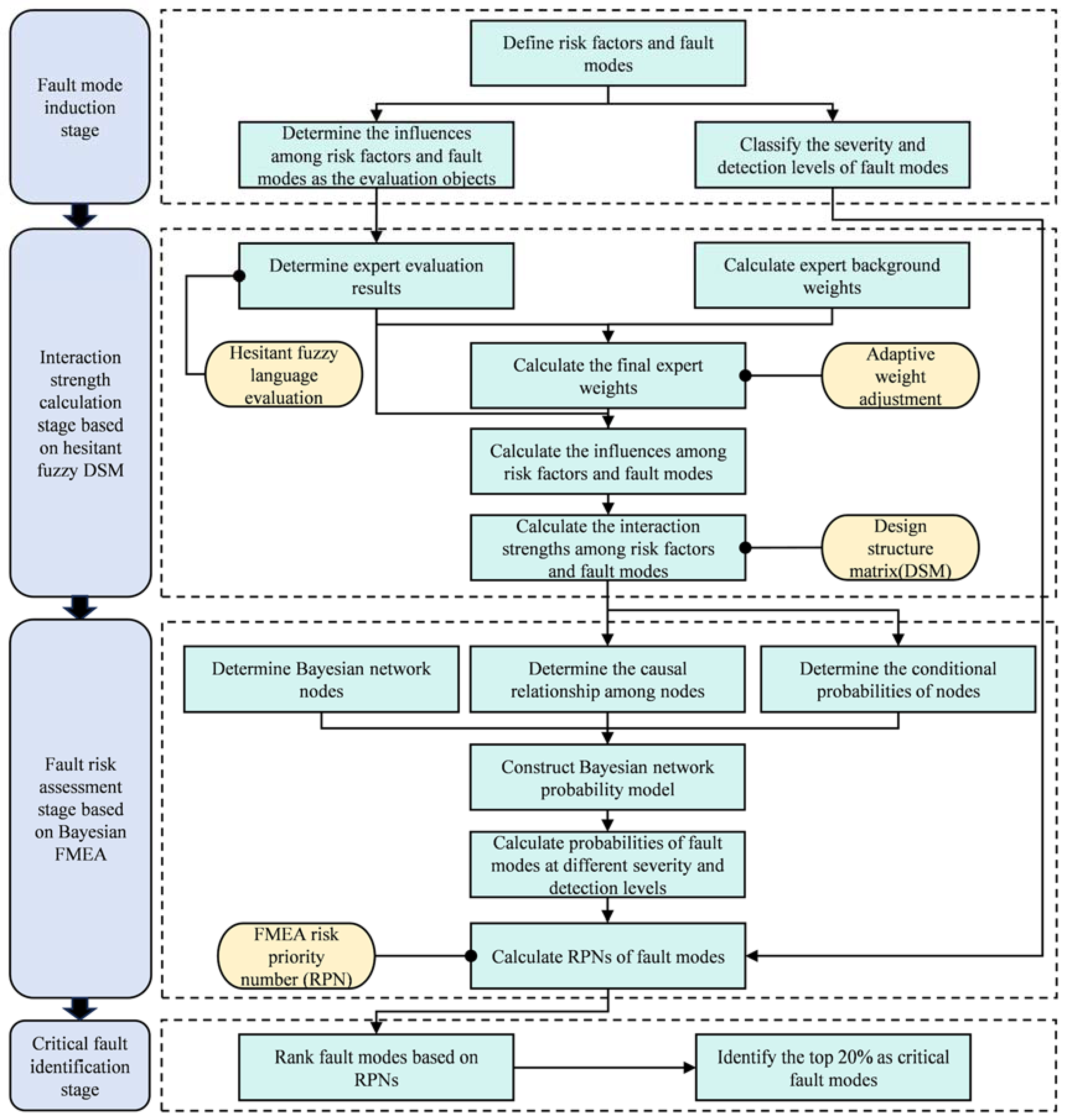
5. Critical Fault Identification and Maintenance Decision-Making Method
5.1. Critical Fault Identification
5.2. Formulation of Maintenance Strategies for Fault Modes
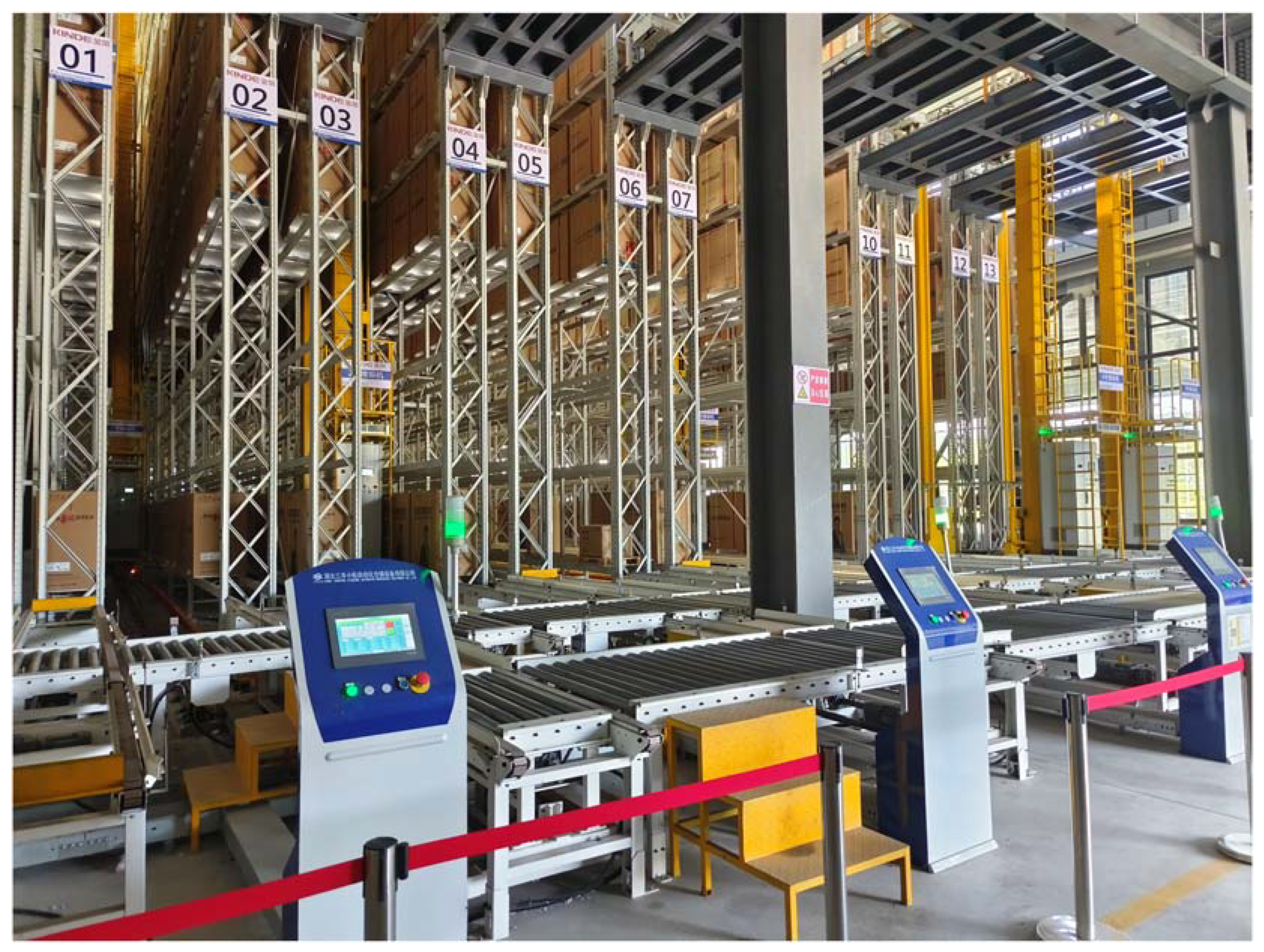
6. Case Study
6.1. Hesitant Fuzzy Evaluation of the Influence
6.2. Interaction Strength Calculation
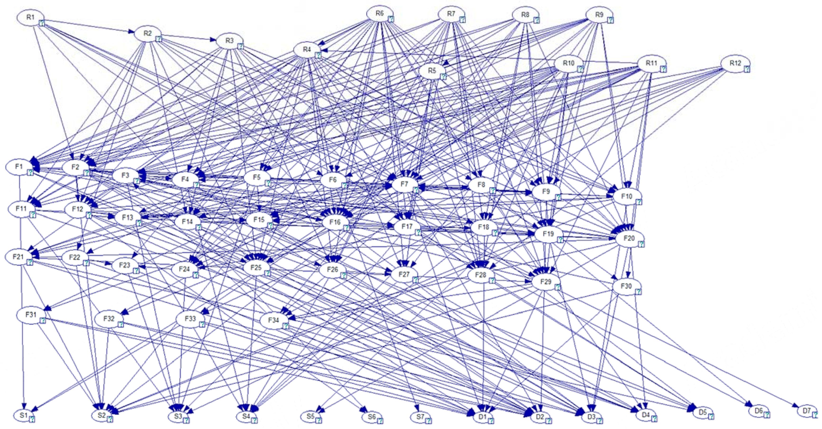
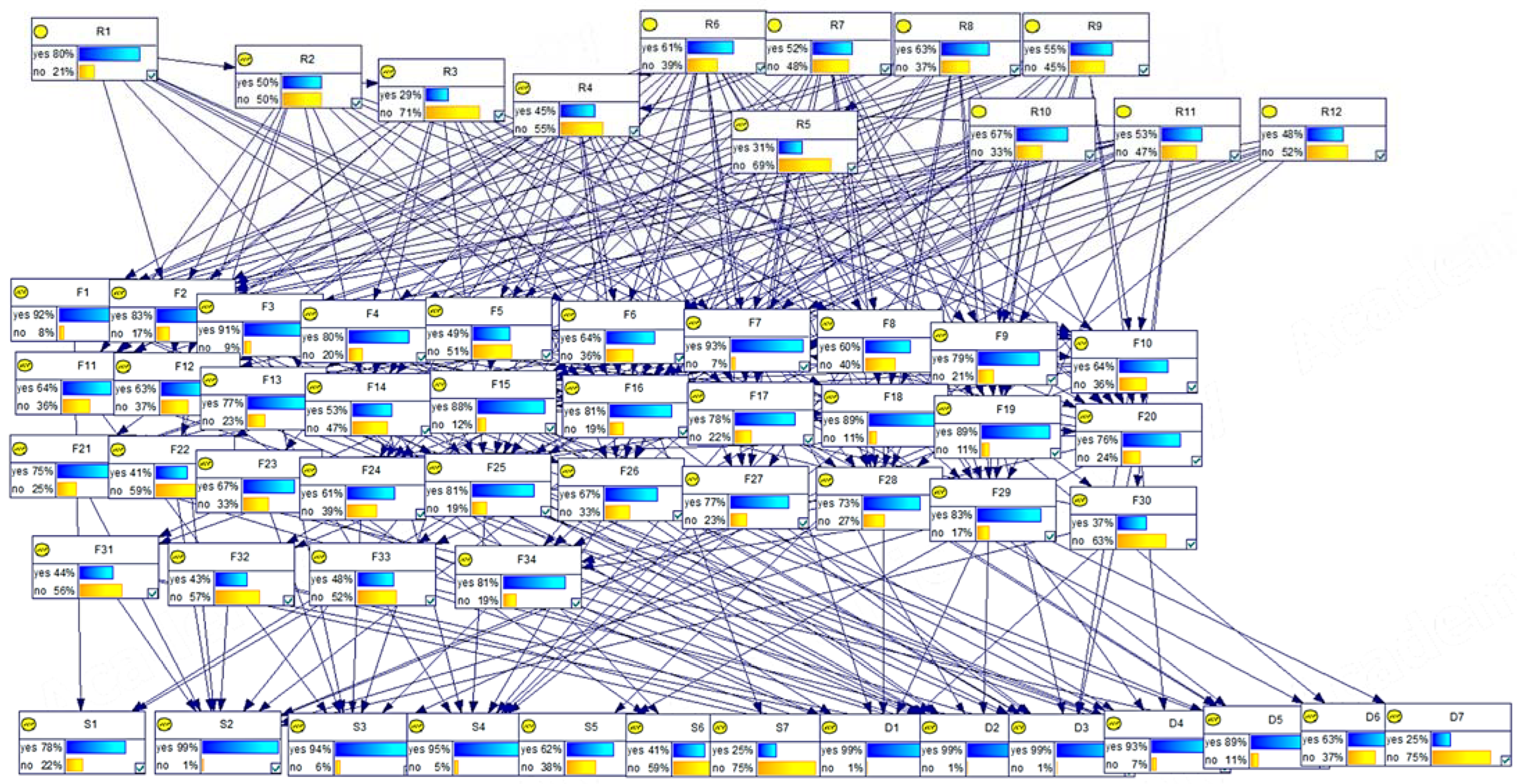
6.3. Probability Calculation of Fault Modes
6.4. Critical Fault Identification and Maintenance Decision-Making
6.5. Results and Analysis
7. Conclusions
Author Contributions
Funding
Data Availability Statement
Conflicts of Interest
Abbreviations
| FMEA | Failure mode and effects analysis |
| DSM | Design structure matrix |
| FTA | Fault tree analysis |
| ETA | Event tree analysis |
| GST | Gray system theory |
| MCS | Monte Carlo simulation |
| RSM | Risk structure matrix |
| AHP | Analytic hierarchy process |
| RPN | Risk priority number |
| O | Occurrence |
| S | Severity |
| D | Detection |
Notations
| Total background score of the th expert | |
| Background weight of the th expert | |
| Evaluation value of the th expert about the influence between the th pair of interacting objects | |
| The th pair of interacting objects group’s weighted average | |
| The th value in hesitant fuzzy numbers | |
| The th value in hesitant fuzzy numbers | |
| The number of values in one hesitant fuzzy number | |
| The difference between the evaluation value of the th expert and the group’s weighted average about the influence between the th pair of interacting objects | |
| Deviation amount of the th expert | |
| Standardized deviation amount of the th expert | |
| Deviation of the th expert | |
| Preprocessed deviation of the th expert | |
| Weight influencing factor of the th expert | |
| Final weight of the th expert is obtained after the th adjustment | |
| The maximum length of all the evaluation sets | |
| The number of th evaluation levels in the evaluation set of the th expert on the influence of the th pair of interacting objects | |
| Trapezoidal fuzzy number of the th evaluation level | |
| Final influence of the th evaluation object with the th evaluation object | |
| Reason vector of the th evaluation object | |
| Influence vector of the th evaluation object | |
| Causal interaction comparison matrix of the th evaluation object | |
| Influence interaction comparison matrix of the th evaluation object | |
| The maximum eigenvectors of the causal interaction comparison matrices for the th evaluation object | |
| The maximum eigenvectors of the influence interaction comparison matrices for the th evaluation object | |
| Reason matrix | |
| Influence matrix | |
| Interaction strength matrix | |
| The th node of Bayesian network | |
| Directed edge among nodes | |
| Conditional probability distributions of nodes | |
| All combinations of parent node states for the th node | |
| The th risk factor | |
| The th fault mode | |
| The th severity level | |
| The th detection level | |
| RPN of the th fault mode | |
| Three-level boundary value |
References
- Li, Z.; Li, M. Design and Implementation of Automated Stereoscopic Warehouse Based on Artificial Intelligence. Adv. Comput. Commun. 2023, 4, 318–323. [Google Scholar] [CrossRef]
- Kuchekar, P.; Bhongade, A.S.; Rehman, A.U.; Mian, S.H. Assessing the Critical Factors Leading to the Failure of the Industrial Pressure Relief Valve Through a Hybrid MCDM-FMEA Approach. Machines 2024, 12, 820. [Google Scholar] [CrossRef]
- Wan, D.; Qiu, H.; Li, M.; Xu, D.; Gao, L. Fuzzy FMEA considering expert consensus and multi-risk factors. Comput. Integr. Manuf. Syst. 2024, 1–22. [Google Scholar]
- Li, Y.; Liu, P.; Li, G. An asymmetric cost consensus based failure mode and effect analysis method with personalized risk attitude information. Reliab. Eng. Syst. Saf. 2023, 235, 109196. [Google Scholar] [CrossRef]
- Huang, G.; Xiao, L.; Zhang, G. Risk evaluation model for failure mode and effect analysis using intuitionistic fuzzy rough number approach. Soft Comput. 2021, 25, 4875–4897. [Google Scholar] [CrossRef]
- Skėrė, S.; Bastida-Molina, P.; Hurtado-Pérez, E.; Juzėnas, K. Energy Consumption Analysis and Efficiency Enhancement in Manufacturing Companies Using Decision Support Method for Dynamic Production Planning (DSM DPP) for Solar PV Integration. Machines 2023, 11, 939. [Google Scholar] [CrossRef]
- Babaleye, A.O.; Kurt, R.E.; Khan, F. Safety analysis of plugging and abandonment of oil and gas wells in uncertain conditions with limited data. Reliab. Eng. Syst. Saf. 2019, 188, 133–141. [Google Scholar] [CrossRef]
- Li, S.; Qin, N.; Huang, D.; Huang, D.; Ke, L. Damage localization of stacker’s track based on EEMD-EMD and DBSCAN cluster algorithms. IEEE Trans. Instrum. Meas. 2019, 69, 1981–1992. [Google Scholar] [CrossRef]
- Xue, G.; Qiao, Y.; Xia, Y.; Li, Y.; Cheng, Z.; Lei, S.; Wang, L. The development and application of online fault waring system for automatic stereo library based with S7-300 and Wincc flexible 2007 operating environment. In Proceedings of the IEEE 9th International Conference on Mechanical and Intelligent Manufacturing Technologies (ICMIMT), Cape Town, South Africa, 10–13 February 2018. [Google Scholar]
- Bao, S.; Zhang, M.; Cai, Z. The slotting optimization of tobacco automated stereoscopic warehouse based on fault tree and field test. In Proceedings of the 2nd IEEE International Conference on Intelligent Transportation Engineering (ICITE), Singapore, 1 September 2019. [Google Scholar]
- Tantau, M.; Popp, E.; Perner, L.; Wielitzka, M.; Ortmaier, T. Model selection ensuring practical identifiability for models of electric drives with coupled mechanics. In Proceedings of the 21st IFAC World Congress on Automatic Control—Meeting Societal Challenges, Berlin, Germany, 11–17 July 2020. [Google Scholar]
- Zhu, Y.; Xu, B.; Su, J.; Fan, Q.; Miao, J. Fault Diagnosis of AS and RS Based on Fuzzy Petri Net. In Proceedings of the Fault Diagnosis of AS and RS Based on Fuzzy Petri Net, Shanghai, China, 12–15 December 2015. [Google Scholar]
- Gnjatovic, N.B.; Urosevic, M.M.; Stefanovic, A.Z.; Bosnjak, S.M.; Zrnic, N.D. Coupled and partial impacts of the inclination angle of the discharge boom and the mass of conveyed material on the dynamic behavior of the stacker superstructure. Mech. Based Des. Struct. Mach. 2024, 1–35. [Google Scholar] [CrossRef]
- Bosnjak, S.M.; Arsic, M.A.; Zrnic, N.D.; Odanovic, Z.D.; Dordevic, M.D. Failure Analysis of the Stacker Crawler Chain Link. In Proceedings of the 11th International Conference on the Mechanical Behavior of Materials (ICM), Como, Italy, 5–9 June 2011. [Google Scholar]
- Qiao, D.; Zhou, X.; Ye, X.; Tang, G.; Lu, L.; Ou, J. Security risk assessment of submerged floating tunnel based on fault tree and multistate fuzzy Bayesian network. Ocean Coastal Manage. 2024, 258, 107355. [Google Scholar] [CrossRef]
- Maidana, R.G.; Parhizkar, T.; San Martin, G.; Utne, I.B. Dynamic probabilistic risk assessment with K-shortest-paths planning for generating discrete dynamic event trees. Reliab. Eng. Syst. Saf. 2024, 242, 109725. [Google Scholar] [CrossRef]
- Chen, X.; Xu, L.; Li, X.; Cong, L. Risk assessment method of power communication network based on gray cloud theory and matter-element extension model coupling. IEEE Access 2023, 12, 47581–47593. [Google Scholar] [CrossRef]
- Zhang, H.; Sun, J.; Tian, Y. Accelerated risk assessment for highly automated vehicles: Surrogate-based monte carlo method. IEEE Trans. Intell. Transp. Syst. 2023, 25, 5488–5497. [Google Scholar] [CrossRef]
- Zhang, P.; Zhang, Z.; Gong, D. An improved normal wiggly hesitant fuzzy FMEA model and its application to risk assessment of electric bus systems. Appl. Intell. 2024, 54, 6213–6237. [Google Scholar] [CrossRef]
- Min, S.; Jang, H. Case Study of Expected Loss Failure Mode and Effect Analysis Model Based on Maintenance Data. Appl. Sci. 2021, 11, 7349. [Google Scholar] [CrossRef]
- Liu, P.; Xu, Y.; Li, Y.; Geng, Y. An FMEA Risk Assessment Method Based on Social Networks Considering Expert Clustering and Risk Attitudes. IEEE Trans. Eng. Manage. 2024, 71, 10783–10796. [Google Scholar] [CrossRef]
- Huang, W.; Zhang, Y. Railway Dangerous Goods Transportation System Risk Assessment: An Approach Combining FMEA With Pessimistic–Optimistic Fuzzy Information Axiom Considering Acceptable Risk Coefficient. IEEE Trans. Reliab. 2021, 70, 371–388. [Google Scholar] [CrossRef]
- Ustundag, A. A Fuzzy Risk Assessment Model for Warehouse Operations. J. Mult.-Valued Log. Soft Comput. 2014, 22, 133–149. [Google Scholar]
- Li, H.; Zhang, Y.H.; Zheng, Y.; Li, L.H. Research of CBR-Based Organizations on Aromourd Equipment Fault-Diagnosis. Appl. Mech. Mater. 2014, 3485, 715–721. [Google Scholar] [CrossRef]
- Salah, B.; Janeh, O.; Bruckmann, T.; Noche, B. Improving the Performance of a New Storage and Retrieval Machine Based on a Parallel Manipulator Using FMEA Analysis. In Proceedings of the 15th IFAC Symposium on Information Control Problems in Manufacturing, Ottawa, Canada, 11–13 May 2015; pp. 1658–1663. [Google Scholar]
- Bevilacqua, M.; Mazzuto, G.; Paciarotti, C. A combined IDEF0 and FMEA approach to healthcare management reengineering. Int. J. Procure. Manage. 2015, 8, 25–43. [Google Scholar] [CrossRef]
- Suwandi, A.; Zagloel, T.Y.; Hidayatno, A. Conceptual model of failure risk control on raw materials inventory system. In Proceedings of the International Conference on Design, Engineering and Computer Sciences (ICDECS), Jakarta, Indonesia, 9 August 2018. [Google Scholar]
- Maslowski, D.; Kulinska, E.; Ltd, T. Analysis of the aoolication of FMEA method of warehouse system in metal foundry. In Proceedings of the 27th International Conference on Metallurgy and Materials (METAL), Brno, Czech Republic, 23–25 May 2018; pp. 2036–2041. [Google Scholar]
- Hassan, A.; Purnomo, M.R.A.; Anugerah, A.R. Fuzzy-analytical-hierarchy process in failure mode and effect analysis (FMEA) to identify process failure in the warehouse of a cement industry. J. Eng. Des. Technol. 2020, 18, 378–388. [Google Scholar] [CrossRef]
- Dewi, I.L.; Pamadya, V.; Tri, P.A.Y. FMEA Approach to Risk Factors as a Factor in Implementing Green Supply Chain Management (Study in PT. Gresik Cipta Sejahtera). J. Phys. Conf. Ser. 2021, 1858, 1. [Google Scholar] [CrossRef]
- Hsu, H.Y.; Hwang, M.H.; Tsou, P.H. Applications of BWM and GRA for Evaluating the Risk of Picking and Material-Handling Accidents in Warehouse Facilities. Appl. Sci. 2023, 13, 1263. [Google Scholar] [CrossRef]
- Esmaeili, S.V.; Alboghobeish, A.; Yazdani, H.; Koozekonan, A.G.; Pouyakian, M. Optimizing in-store warehouse safety: A DEMATEL approach to comprehensive risk assessment. PLoS ONE 2025, 20, e0317787. [Google Scholar] [CrossRef]
- Huang, X.; Gui, P.; Yao, J.; Zhu, W.; Zhou, C.; Li, X.; Li, S. An Applied View to Determine the Weights of Experts’ Scores Based on an Evidential Reasoning Approach Under Two-Dimensional Frameworks. IAENG Int. J. Comput. Sci. 2023, 50, 970–979. [Google Scholar]
- Hernández-Fernández, L.; Vázquez, J.G.; Hernández, L.; Campbell, R.; Martínez, J.; Hajari, E.; González-De Zayas, R.; Zevallos-Bravo, B.E.; Acosta, Y.; Lorenzo, J.C. Use of Euclidean distance to evaluate Pistia stratiotes and Eichhornia crassipes as organic fertilizer amendments in Capsicum annuum. Acta Physiol. Plant. 2024, 46, 21. [Google Scholar] [CrossRef]
- Lu, H.; Bai, Q.; Meng, F. Joint production and sustainability investment decisions for a risk-averse manufacturer under a Cap-and-trade policy. Sustain. Oper. Comput. 2024, 5, 131–140. [Google Scholar] [CrossRef]
- Özdemir, A.; Uçurum, M.; Serencam, H. A novel fuzzy cumulative sum control chart with an α-level cut based on trapezoidal fuzzy numbers for a real case application. Arab. J. Sci. Eng. 2024, 49, 7507–7525. [Google Scholar] [CrossRef]
- Wu, Z.; Li, Y.; Jing, Q. Quantitative risk assessment of coal mine gas explosion based on a Bayesian network and computational fluid dynamics. Process Saf. Environ. Protect. 2024, 190, 780–793. [Google Scholar] [CrossRef]
- Feng, X.; Jiang, J.; Wang, W. Gas pipeline failure evaluation method based on a Noisy-OR gate bayesian network. J. Loss Prev. Process Ind. 2020, 66, 104175. [Google Scholar] [CrossRef]
- Samal, N.; Ashwin, R.; Singhal, A.; Jha, S.K.; Robertson, D.E. Using a Bayesian joint probability approach to improve the skill of medium-range forecasts of the Indian summer monsoon rainfall. J. Hydrol. Reg. Stud. 2023, 45, 101284. [Google Scholar] [CrossRef]
- Zhang, H.; Liu, S.; Dong, Y.; Chiclana, F.; Herrera-Viedma, E.E. A minimum cost consensus-based failure mode and effect analysis framework considering experts’ limited compromise and tolerance behaviors. IEEE T. Cybern. 2022, 53, 6612–6625. [Google Scholar] [CrossRef] [PubMed]
- Rakyta, M.; Bubenik, P.; Binasova, V.; Gabajova, G.; Staffenova, K. The Change in Maintenance Strategy on the Efficiency and Quality of the Production System. Electronics 2024, 13, 3449. [Google Scholar] [CrossRef]
- Omshi, E.M.; Shemehsavar, S.; Grall, A. An intelligent maintenance policy for a latent degradation system. Reliab. Eng. Syst. Saf. 2024, 242, 109739. [Google Scholar] [CrossRef]
- Liu, P.; Wang, G.; Tan, Z.-H. Calendar-time-based and age-based maintenance policies with different repair assumptions. Appl. Math. Model. 2024, 129, 592–611. [Google Scholar] [CrossRef]
- Li, X.; Ran, Y.; Fafa, C.; Zhu, X.; Wang, H.; Zhang, G. A maintenance strategy selection method based on cloud DEMATEL-ANP. Soft Comput. 2023, 27, 18843–18868. [Google Scholar] [CrossRef]
- De Jonge, B.; Scarf, P.A. A review on maintenance optimization. Eur. J. Oper. Res. 2020, 285, 805–824. [Google Scholar] [CrossRef]
- Cheikh, K.; Boudi, E.M.; Rabi, R.; Mokhliss, H. Balancing the maintenance strategies to making decisions using Monte Carlo method. MethodsX 2024, 13, 102819. [Google Scholar] [CrossRef]
- Aafif, Y.; Schutz, J.; Dellagi, S.; Chelbi, A.; Mifdal, L. Integrated design and maintenance strategies for wind turbine gearboxes. J. Qual. Maint. Eng. 2024, 30, 521–539. [Google Scholar] [CrossRef]
- Godoy, D.R.; Álvarez, V.; Mena, R.; Viveros, P.; Kristjanpoller, F. Adopting New Machine Learning Approaches on Cox’s Partial Likelihood Parameter Estimation for Predictive Maintenance Decisions. Machines 2024, 12, 60. [Google Scholar] [CrossRef]
- Lefebvre, M.; Yaghoubi, R. Optimal Inspection and Maintenance Policy: Integrating a Continuous-Time Markov Chain into a Homing Problem. Machines 2024, 12, 795. [Google Scholar] [CrossRef]
- Esa, M.A.M.; Muhammad, M. Adoption of prescriptive analytics for naval vessels risk-based maintenance: A conceptual framework. Ocean Eng. 2023, 278, 114409. [Google Scholar] [CrossRef]
- Cicek, K.; Celik, M. Application of failure modes and effects analysis to main engine crankcase explosion failure on-board ship. Saf. Sci. 2013, 51, 6–10. [Google Scholar] [CrossRef]
- Kuang, Y.; Zou, S.; Tang, D. Risk analysis for the used or spent fuel shearing machine based on the fuzzy FMEA. J. Saf. Environ. 2016, 16, 15–20. [Google Scholar] [CrossRef]


| Author | Year | Research Target | Method | Application |
|---|---|---|---|---|
| Ustundag et al. [23] | 2012 | SCM warehouse | Fuzzy-FMEA | Fault risk assessment |
| Li et al. [24] | 2014 | Equipment warehouse | CBR-FMEA | Fault risk assessment |
| Salah et al. [25] | 2015 | Automated warehouse | Traditional FMEA | Optimized parameters for system reliability |
| Bevilacqua et al. [26] | 2015 | Pharmacy warehouse | IDEF0-FMEA | Fault risk assessment |
| Adriansyah et al. [27] | 2018 | Materials warehouse | SD-FMEA | Continuous improvement of the system of risk control |
| Maslowski et al. [28] | 2018 | Warehouse | Traditional FMEA | Find the causes of defects, to commit repair tasks |
| Hassan et al. [29] | 2019 | Cement industry warehouse | Fuzzy-analytical-hierarchy FMEA | Fault risk assessment |
| Indrasari et al. [30] | 2021 | Green SCM warehouse | Traditional FMEA | Fault risk assessment |
| Hsu et al. [31] | 2023 | Warehouse | BWM-FMEA | Fault risk assessment |
| Esmaeili et al. [32] | 2025 | Instore warehouse | DEMATEL-FMEA | Fault risk assessment |
| Position | Educational Level | Work Experience | Age | Familiarity Level | Score |
|---|---|---|---|---|---|
| General operators | Junior college below | 1–5 years | 20–25 | Understand | 1 |
| Technician | Junior college | 6–10 years | 25–30 | Between understanding and familiar | 2 |
| Junior researcher | Undergraduate | 11–20 years | 31–40 | Familiar | 3 |
| Senior researcher | Master | 20–30 years | 41–50 | Between familiar and very familiar | 4 |
| Senior expert | Doctor | 30–40 years | 50–60 | Very familiar | 5 |
| Level | Severity Number | Level Definition | Detection Number | Level Definition | Score |
|---|---|---|---|---|---|
| 1 | S1 | The influence is minimal, with no significant effect on system operation or security | D1 | Detection is simple through routine checks or monitoring systems | 1 |
| 2 | S2 | The system remains unaffected and needs only minor adjustments | D2 | Easily detectable but needs specific testing methods | 2 |
| 3 | S3 | The system’s operational efficiency slightly decreases, allowing for quick repairs | D3 | Moderately detectable, requiring professional tools for inspection or analysis | 3 |
| 4 | S4 | The issue partially affects a single device, which can be restored with backups or simple repairs, and has minimal impact on the overall system | D4 | Detection is difficult and requires complex testing or advanced analysis | 4 |
| 5 | S5 | The issue leads to a partial system shutdown, causing longer maintenance and moderate effects on production plans | D5 | Detection is challenging and requires expertise and specialized equipment | 5 |
| 6 | S6 | The malfunction of critical equipment components has restricted system operations, adversely affecting production goals | D6 | Detection is rather challenging and requires advanced technology | 6 |
| 7 | S7 | The malfunction of critical equipment has caused system failures and extended repair times, greatly affecting production | D7 | Detection and prediction are nearly impossible until serious consequences occur | 7 |
| Level | Relationship Representation | Trapezoidal Fuzzy Number | Language Evaluation |
|---|---|---|---|
| 0 | N | (0, 0, 0, 0) | No influence |
| 1 | L | (0, 1, 1, 2) | Low influence |
| 2 | BLM | (2, 3, 3, 4) | Between low and moderate influence |
| 3 | M | (4, 5, 5, 6) | Moderate influence |
| 4 | BMH | (6, 7, 7, 8) | Between moderate and high influence |
| 5 | H | (8, 8, 9, 9) | High influence |
| 6 | VH | (9, 9, 10, 10) | Very high influence |
| Maintenance Strategy | Fault Risk Level |
|---|---|
| Condition-based maintenance | |
| Periodic maintenance | |
| Breakdown maintenance |
| Equipment Name | Brand Selection | Equipment Name | Brand Selection | ||
|---|---|---|---|---|---|
| Rack system | Rack | Main material Q355B, other materials Q235B, 14 × 14 | Stacker system | Shuttle | MIAS/LHD/Apes Fork |
| Storage location | 1130 mm × 670 mm × 1200 mm | Wire rope | German Pfeifer | ||
| Stacker system | Stacker | Double-extension double-mast single-station stacker | VFD | Siemens/Schneider | |
| Ground rail | 30 kg | Transportation system | Motor | SEW/NORD | |
| Ceiling rail | 100 mm × 100 mm × 10 mm Angle steel | VFD | Siemens /Danfoss | ||
| Sliding rail | Panasonic /Vahle | Detection device | OMRON | ||
| Travelling addressing system | German Sick/Leuze | Low-voltage apparatus | Schneider | ||
| Lifting addressing system | German Sick | Conveyor chain | Hangzhou Donghua /Anhui Huangshan | ||
| Critical position bearing | Swedish SKF/NSK | Drive chain | Hangzhou Donghua/Anhui Huangshan | ||
| Travelling wheel | Komatsu | Bearing part | Dongguan Bearing factory/Haerbin Bearing factory, TR/SKF | ||
| Motor | SEW | Lamp | Schneider/APT | ||
| Number | Fault Mode | Number | Fault Mode |
|---|---|---|---|
| F1 | Noise | F18 | Break of wire rope of the stacker lifting mechanism |
| F2 | Mechanical wear of ground rail | F19 | Abnormal pulling marks on the guiding rail of the stacker lifting mechanism |
| F3 | Addressing fault of stacker shuttle | F20 | Stacker motor overheating |
| F4 | Shaking of stacker frame beam | F21 | Stacker shuttle exceeds the limit |
| F5 | Fault of laser rangefinder of stacker horizontal travelling mechanism | F22 | Stacker shuttle shaking |
| F6 | Cracks in the weld seam of stacker mast | F23 | Stacker shuttle timeout |
| F7 | Damage of travelling wheels of stacker horizontal travelling mechanism | F24 | Stacker shuttle does not extend smoothly |
| F8 | Stuck of stacker guiding wheels | F25 | Break of conveyor chain of transportation system |
| F9 | Clearance or separation of stacker guiding wheels | F26 | Stuck or leaking of conveyor chain of transportation system |
| F10 | Damage of stacker reducer | F27 | Unstable conveyor belt of transportation system |
| F11 | Damage of stacker VDF | F28 | Fault of forklift operation of transportation system |
| F12 | Damage of stacker brake | F29 | Damage of rack |
| F13 | Tripping of stacker control switch | F30 | Settlement of rack |
| F14 | Damage of stacker limiting switch | F31 | Empty pickup and empty outbound |
| F15 | Position deviation of stacker horizontal travelling mechanism | F32 | Double storage and double unloading |
| F16 | Damage of rope winding device of stacker lifting mechanism | F33 | Fault of scanning device |
| F17 | Damage of stacker lifting mechanism | F34 | The stacking type of goods in the rack is not standardized |
| Number | Risk Factor | Number | Risk Factor |
|---|---|---|---|
| R1 | Is the material qualified? | R7 | Is the maintenance strategy reasonable? |
| R2 | Is the quality of the parts qualified? | R8 | Work overload |
| R3 | Is the quality of the assembly qualified? | R9 | Variable workload |
| R4 | Equipment aging or long service life | R10 | Improper operation by workers |
| R5 | Equipment damage | R11 | Is the operating environment suitable? |
| R6 | Is the equipment regularly maintained? | R12 | Is the information system functioning properly? |
| Number | Position | Educational Level | Work Experience | Age | Familiarity Level | Score | Background Weights |
|---|---|---|---|---|---|---|---|
| 1 | General operators | Undergraduate | 1–5 years | 20–25 | Familiar | 9 | 0.117 |
| 2 | Technician | Master | 1–5 years | 25–30 | Between understanding and familiar | 11 | 0.143 |
| 3 | Junior researcher | Master | 6–10 years | 25–30 | Familiar | 14 | 0.182 |
| 4 | Senior researcher | Doctor | 11–20 years | 31–40 | Very familiar | 20 | 0.26 |
| 5 | Senior expert | Doctor | 20–30 years | 50–60 | Between familiar and very familiar | 23 | 0.299 |
| Number | Risk Factor | Expert Evaluation Level | ||||
|---|---|---|---|---|---|---|
| 1 | 2 | 3 | 4 | 5 | ||
| 1 | R1→R2 | 6 | 5 | 4 | 4, 5 | 4, 5 |
| 2 | R2→R3 | 4, 5 | 4 | 5 | 3, 4 | 4 |
| 3 | R6→R4 | 5 | 5 | 5, 6 | 4 | 5 |
| 4 | R11→R4 | 3 | 2, 3 | 3 | 3, 4 | 4 |
| 5 | R8→R5 | 4 | 3, 4 | 3 | 3 | 3 |
| Expert Number | Final Weights of Experts | ||
|---|---|---|---|
| When Evaluating the Interactions Among Risk Factors | When Evaluating the Interactions Among Risk Factors and Fault Modes | When Evaluating the Interactions Among Fault Modes | |
| 1 | 0.081 | 0.101 | 0.092 |
| 2 | 0.131 | 0.120 | 0.136 |
| 3 | 0.147 | 0.163 | 0.155 |
| 4 | 0.258 | 0.248 | 0.244 |
| 5 | 0.384 | 0.368 | 0.374 |
| P (F/S, D) | Value | P (F/S, D) | Value | P(F/S, D) | Value |
|---|---|---|---|---|---|
| P (F1/S1, D4) | 0.95 | P (F12/S6, D2) | 0.861 | P (F22/S2, D2) | 0.41 |
| P (F1/S1, D3) | 0.941 | P (F12/S6, D4) | 0.868 | P (F23/S3, D1) | 0.698 |
| P (F2/S2, D3) | 0.835 | P (F13/S4, D4) | 0.811 | P (F24/S3, D2) | 0.635 |
| P (F2/S2, D1) | 0.834 | P (F13/S4, D2) | 0.788 | P (F25/S4, D2) | 0.824 |
| P (F3/S3, D5) | 0.934 | P (F14/S6, D5) | 0.724 | P (F26/S4, D2) | 0.687 |
| P (F4/S4, D2) | 0.822 | P (F14/S6, D2) | 0.709 | P (F27/S4, D4) | 0.795 |
| P (F4/S4, D3) | 0.822 | P (F15/S2, D4) | 0.899 | P (F28/S3, D5) | 0.755 |
| P (F5/S3, D3) | 0.511 | P (F15/S2, D3) | 0.888 | P (F29/S2, D1) | 0.839 |
| P (F6/S7, D7) | 1 | P (F16/S1, D3) | 0.887 | P (F30/S2, D1) | 0.374 |
| P (F7/S2, D2) | 0.945 | P (F17/S4, D5) | 0.818 | P (F31/S2, D1) | 0.447 |
| P (F7/S2, D1) | 0.943 | P (F17/S4, D6) | 0.922 | P (F31/S2, D2) | 0.445 |
| P (F7/S2, D5) | 0.947 | P (F18/S4, D1) | 0.902 | P (F32/S2, D1) | 0.432 |
| P (F8/S4, D4) | 0.631 | P (F19/S2, D3) | 0.897 | P (F32/S2, D2) | 0.43 |
| P (F8/S4, D6) | 0.707 | P (F20/S5, D4) | 0.909 | P (F33/S1, D1) | 0.544 |
| P (F9/S5, D2) | 0.862 | P (F20/S5, D3) | 0.902 | P (F33/S1, D3) | 0.542 |
| P (F10/S2, D3) | 0.645 | P (F21/S2, D2) | 0.757 | P (F34/S3, D1) | 0.846 |
| P (F11/S3, D4) | 0.674 | P (F21/S2, D5) | 0.785 | P (F34/S3, D3) | 0.844 |
| Fault Mode | Probability | Severity | Detection | RPN | Total RPN | Ranking | |
|---|---|---|---|---|---|---|---|
| F1 | P (F1/S1, D4) | 0.95 | 1 | 4 | 3.8 | 6.623 | 19 |
| P (F1/S1, D3) | 0.941 | 1 | 3 | 2.823 | |||
| F2 | P (F2/S2, D3) | 0.835 | 2 | 3 | 5.01 | 6.678 | 18 |
| P (F2/S2, D1) | 0.834 | 2 | 1 | 1.668 | |||
| F3 | P (F3/S3, D5) | 0.934 | 3 | 5 | 14.01 | 14.01 | 10 |
| F4 | P (F4/S4, D2) | 0.822 | 4 | 2 | 6.576 | 16.44 | 8 |
| P (F4/S4, D3) | 0.822 | 4 | 3 | 9.864 | |||
| F5 | P (F5/S3, D3) | 0.511 | 3 | 3 | 4.599 | 4.599 | 23 |
| F6 | P (F6/S7, D7) | 1 | 7 | 7 | 49 | 49 | 1 |
| F7 | P (F7/S2, D2) | 0.945 | 2 | 2 | 3.78 | 15.136 | 9 |
| P (F7/S2, D1) | 0.943 | 2 | 1 | 1.886 | |||
| P (F7/S2, D5) | 0.947 | 2 | 5 | 9.47 | |||
| F8 | P (F8/S4, D4) | 0.631 | 4 | 4 | 10.096 | 27.064 | 6 |
| P (F8/S4, D6) | 0.707 | 4 | 6 | 16.968 | |||
| F9 | P (F9/S5, D2) | 0.862 | 5 | 2 | 8.62 | 8.62 | 16 |
| F10 | P (F10/S2, D3) | 0.645 | 2 | 3 | 3.87 | 3.87 | 24 |
| F11 | P (F11/S3, D4) | 0.674 | 3 | 4 | 8.088 | 8.088 | 17 |
| F12 | P (F12/S6, D2) | 0.861 | 6 | 2 | 10.332 | 31.164 | 4 |
| P (F12/S6, D4) | 0.868 | 6 | 4 | 20.832 | |||
| F13 | P (F13/S4, D4) | 0.811 | 4 | 4 | 12.976 | 19.28 | 7 |
| P (F13/S4, D2) | 0.788 | 4 | 2 | 6.304 | |||
| F14 | P (F14/S6, D5) | 0.724 | 6 | 5 | 21.72 | 30.228 | 5 |
| P (F14/S6, D2) | 0.709 | 6 | 2 | 8.508 | |||
| F15 | P (F15/S2, D4) | 0.899 | 2 | 4 | 7.192 | 12.52 | 12 |
| P (F15/S2, D3) | 0.888 | 2 | 3 | 5.328 | |||
| F16 | P (F16/S1, D3) | 0.887 | 1 | 3 | 2.661 | 2.661 | 28 |
| F17 | P (F17/S4, D5) | 0.818 | 4 | 5 | 16.36 | 38.488 | 2 |
| P (F17/S4, D6) | 0.922 | 4 | 6 | 22.128 | |||
| F18 | P (F18/S4, D1) | 0.902 | 4 | 1 | 3.608 | 3.608 | 26 |
| F19 | P (F19/S2, D3) | 0.897 | 2 | 3 | 5.382 | 5.382 | 22 |
| F20 | P (F20/S5, D4) | 0.909 | 5 | 4 | 18.18 | 31.71 | 3 |
| P (F20/S5, D3) | 0.902 | 5 | 3 | 13.53 | |||
| F21 | P (F21/S2, D2) | 0.757 | 2 | 2 | 3.028 | 10.878 | 14 |
| P (F21/S2, D5) | 0.785 | 2 | 5 | 7.85 | |||
| F22 | P (F22/S2, D2) | 0.41 | 2 | 2 | 1.64 | 1.64 | 33 |
| F23 | P (F23/S3, D1) | 0.698 | 3 | 1 | 2.094 | 2.094 | 31 |
| F24 | P (F24/S3, D2) | 0.635 | 3 | 2 | 3.81 | 3.81 | 25 |
| F25 | P (F25/S4, D2) | 0.824 | 4 | 2 | 6.592 | 6.592 | 20 |
| F26 | P (F26/S4, D2) | 0.687 | 4 | 2 | 5.496 | 5.496 | 21 |
| F27 | P (F27/S4, D4) | 0.795 | 4 | 4 | 12.72 | 12.72 | 11 |
| F28 | P (F28/S3, D5) | 0.755 | 3 | 5 | 11.325 | 11.325 | 13 |
| F29 | P (F29/S2, D1) | 0.839 | 2 | 1 | 1.678 | 1.678 | 32 |
| F30 | P (F30/S2, D1) | 0.374 | 2 | 1 | 0.748 | 0.748 | 34 |
| F31 | P (F31/S2, D1) | 0.447 | 2 | 1 | 0.894 | 2.674 | 27 |
| P (F31/S2, D2) | 0.445 | 2 | 2 | 1.78 | |||
| F32 | P (F32/S2, D1) | 0.432 | 2 | 1 | 0.864 | 2.584 | 29 |
| P (F32/S2, D2) | 0.43 | 2 | 2 | 1.72 | |||
| F33 | P (F33/S1, D1) | 0.544 | 1 | 1 | 0.544 | 2.17 | 30 |
| P (F33/S1, D3) | 0.542 | 1 | 3 | 1.626 | |||
| F34 | P (F34/S3, D1) | 0.846 | 3 | 1 | 2.538 | 10.134 | 15 |
| P (F34/S3, D3) | 0.844 | 3 | 3 | 7.596 | |||
| Maintenance Strategy | RPN | Fault Modes |
|---|---|---|
| Condition-based maintenance | (32.916, 49] | F6, F17 |
| Periodic maintenance | (16.832, 32.916] | F8, F12, F13, F14, F20 |
| Breakdown maintenance | [0.748, 16.832] | F1, F2, F3, F4, F5, F7, F9, F10, F11, F15, F16, F18, F19, F21, F22, F23, F24, F25, F26, F27, F28, F29, F30, F31, F32, F33, F34 |
| Fault Mode | Description | RPN | Maintenance Strategy |
|---|---|---|---|
| F6 | Cracks in the weld seam of stacker mast | 49.000 | Condition-based maintenance |
| F17 | Damage of stacker lifting mechanism | 38.488 | Condition-based maintenance |
| F20 | Stacker motor overheating | 31.710 | Periodic maintenance |
| F12 | Damage of stacker brake | 31.164 | Periodic maintenance |
| F14 | Damage of stacker limiting switch | 30.228 | Periodic maintenance |
| F8 | Stuck of stacker guiding wheels | 27.064 | Periodic maintenance |
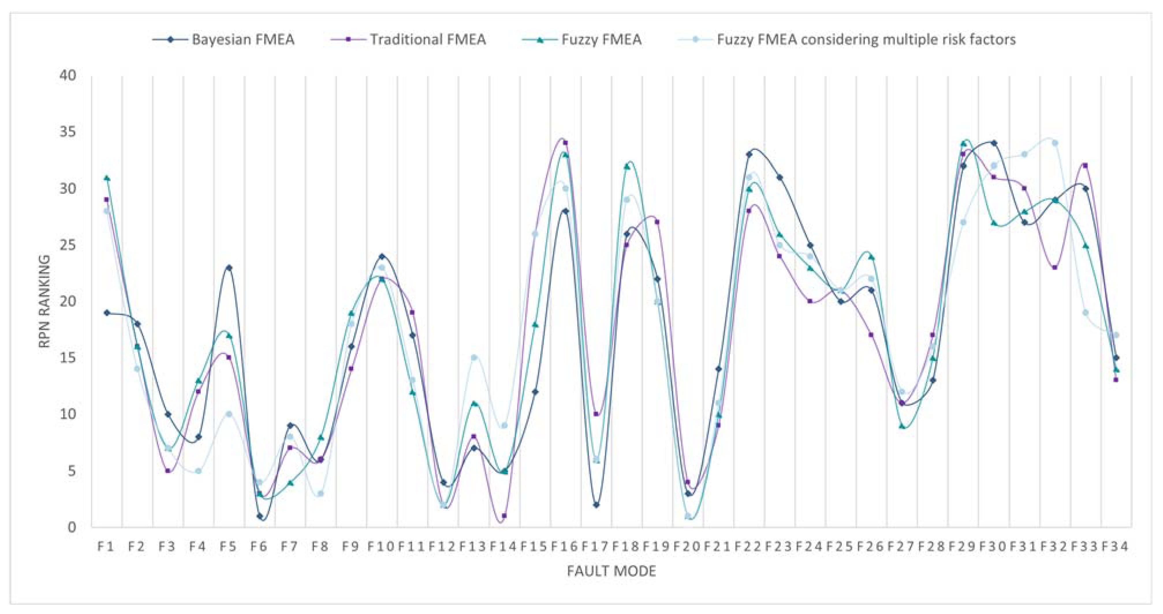
| Fault Mode | Bayesian FMEA | Traditional FMEA | Fuzzy FMEA | Fuzzy FMEA Considering Multiple Risk Factors | Fault Mode | Bayesian FMEA | Traditional FMEA | Fuzzy FMEA | Fuzzy FMEA Considering Multiple Risk Factors |
|---|---|---|---|---|---|---|---|---|---|
| F1 | 19 | 29 | 31 | 28 | F18 | 26 | 25 | 32 | 29 |
| F2 | 18 | 16 | 16 | 14 | F19 | 22 | 27 | 20 | 20 |
| F3 | 10 | 5 | 7 | 7 | F20 | 3 | 4 | 1 | 1 |
| F4 | 8 | 12 | 13 | 5 | F21 | 14 | 9 | 10 | 11 |
| F5 | 23 | 15 | 17 | 10 | F22 | 33 | 28 | 30 | 31 |
| F6 | 1 | 3 | 3 | 4 | F23 | 31 | 24 | 26 | 25 |
| F7 | 9 | 7 | 4 | 8 | F24 | 25 | 20 | 23 | 24 |
| F8 | 6 | 6 | 8 | 3 | F25 | 20 | 21 | 21 | 21 |
| F9 | 16 | 14 | 19 | 18 | F26 | 21 | 17 | 24 | 22 |
| F10 | 24 | 22 | 22 | 23 | F27 | 11 | 11 | 9 | 12 |
| F11 | 17 | 19 | 12 | 13 | F28 | 13 | 17 | 15 | 16 |
| F12 | 4 | 2 | 2 | 2 | F29 | 32 | 33 | 34 | 27 |
| F13 | 7 | 8 | 11 | 15 | F30 | 34 | 31 | 27 | 32 |
| F14 | 5 | 1 | 5 | 9 | F31 | 27 | 30 | 28 | 33 |
| F15 | 12 | 26 | 18 | 26 | F32 | 29 | 23 | 29 | 34 |
| F16 | 28 | 34 | 33 | 30 | F33 | 30 | 32 | 25 | 19 |
| F17 | 2 | 10 | 6 | 6 | F34 | 15 | 13 | 14 | 17 |
Disclaimer/Publisher’s Note: The statements, opinions and data contained in all publications are solely those of the individual author(s) and contributor(s) and not of MDPI and/or the editor(s). MDPI and/or the editor(s) disclaim responsibility for any injury to people or property resulting from any ideas, methods, instructions or products referred to in the content. |
© 2025 by the authors. Licensee MDPI, Basel, Switzerland. This article is an open access article distributed under the terms and conditions of the Creative Commons Attribution (CC BY) license (https://creativecommons.org/licenses/by/4.0/).
Share and Cite
Ma, X.; Gu, M. A Bayesian FMEA-Based Method for Critical Fault Identification in Stacker-Automated Stereoscopic Warehouses. Machines 2025, 13, 242. https://doi.org/10.3390/machines13030242
Ma X, Gu M. A Bayesian FMEA-Based Method for Critical Fault Identification in Stacker-Automated Stereoscopic Warehouses. Machines. 2025; 13(3):242. https://doi.org/10.3390/machines13030242
Chicago/Turabian StyleMa, Xinyue, and Mengyao Gu. 2025. "A Bayesian FMEA-Based Method for Critical Fault Identification in Stacker-Automated Stereoscopic Warehouses" Machines 13, no. 3: 242. https://doi.org/10.3390/machines13030242
APA StyleMa, X., & Gu, M. (2025). A Bayesian FMEA-Based Method for Critical Fault Identification in Stacker-Automated Stereoscopic Warehouses. Machines, 13(3), 242. https://doi.org/10.3390/machines13030242