Improved A* Algorithm-Based Optimal Path Planning of Rescue Robots Within Multi-Environment Maps

Abstract

The traditional A* algorithm performs well in single-map environments, but it is prone to path redundancy and obstacle handling delays in complex multi-map collaborative scenarios, making it unsuitable for the characteristics of multi-environment maps. To address these challenges of traditional A* algorithms, this paper proposes a multi-environment map rescue robot path planning method based on an improved A* algorithm. This method introduces an expected cost evaluation function to achieve weighted fusion of path costs and heuristic values from multiple maps, allowing the algorithm to integrate obstacle distributions and weight information across different environments. A random obstacle replacement mechanism is further designed to maintain path feasibility by locally substituting blocked nodes with adjacent accessible nodes, thereby ensuring continuity without global replanning. Through the combination of multi-map information fusion and local obstacle handling, the algorithm generates a globally optimized path that balances planning efficiency, robustness, and adaptability in uncertain rescue scenarios. Experiment results for a 50 × 50 map scenario show that the improved algorithm significantly outperforms single-map planning results in terms of path redundancy, total length, and turning characteristics. The expansion experiments demonstrate that the paths planned by the proposed algorithm are highly consistent with the optimal paths in terms of direction and local deviations, verifying its good feasibility and effectiveness.

1. Introduction

Natural disasters and sudden accidents pose severe threats to human life and safety. In recent years, with advancements in technology, artificial intelligence devices have been employed to perform high-risk tasks, leading to the increasing application of robots in post-disaster rescue operations. Path planning is a pivotal component in rescue robotics, where environmental mapping accuracy and solution efficiency for optimal path planning problems critically determine mission success in search, detection, and response operations of rescue robots [1].

Environment map modeling is the initial but important step of optimal path planning for rescue robots, which is also critical for improving the efficiency and stability of path planning. Grid-based maps, as one of the most widely used and accepted methods for environmental modeling, have been extensively applied in robot path planning. However, they face significant challenges when dealing with unstructured rescue environments. To represent complex terrain elevation and the distribution of dynamic obstacles, resulting in insufficient path safety and low planning efficiency, researchers have proposed various map processing strategies. Liu et al. [2] introduced a hybrid map model combining 2D grids with 2.5D elevation information, significantly enhancing a robot’s traversability assessment in unstructured terrain. Xie et al. [3] proposed an A* algorithm based on a 2.5D navigation map, simplifying obstacles in 3D environments into cuboids by partitioning the XOZ plane, thereby improving adaptability to complex three-dimensional environments. Li et al. [4] converted non-standard maps into standard grid maps using calibration markers and integrated an ant colony algorithm to achieve path planning in unstructured environments. Lee et al. [5] introduced a wavefront propagation map model (TRG) based on terrain geometric traversability, optimizing both safety and path distance efficiency in unstructured environments through hierarchical management of node stability and reachability. Zhao and Hwang [6] proposed a grid map modeling method based on subregion division, decomposing the map into minimal units and constructing tree-like branches to enhance global coverage efficiency. Lu et al. [7] segmented the map into uniformly sized “brick” units, mapped them into bipartite graph nodes, and selected non-overlapping coverage regions via the maximum independent set (MIS), reducing turning frequency and cutting task completion time by 22%. Sun et al. [8] developed a virtual obstacle search method for wheel-legged robots by partitioning the map into body and wheel maps, addressing path planning challenges for reconfigurable robots. Although these map modeling methods significantly improve path planning through multi-dimensional information fusion and hierarchical processing, most focus on optimizing single maps and lack adaptive optimization for obstacle types and inter-map correlations in multi-map fusion, leading to imbalanced obstacle representation and map information utilization in complex scenarios [9]. Despite grid-based mapping having demonstrated significant success in unstructured environment modeling, its application in complex rescue scenarios remains constrained by limitations in sensing technologies and field equipment, often resulting in incomplete environmental data. Under such conditions, it becomes critically important to incorporate obstacle distribution characteristics and risk factors by leveraging prior knowledge and expert experience. This approach enables probabilistic prediction of obstacle configurations, generating multiple environment maps with subjective probability estimates for robotic path planning. Such methodology holds substantial implications for enhancing rescue efficiency and reducing operational timeframes in disaster response missions.

The development of path planning solvers represents a fundamental research direction in rescue robot navigation, having evolved from traditional heuristic approaches, such as A* [10], Dijkstra’s Algorithm (Dijkstra) [11], Rapidly exploring Random Tree (RRT) [12] to contemporary intelligent methods including bio-inspired optimization, such as Particle Swarm Optimization (PSO) [13], Genetic Algorithm (GA) [14], Ant Colony Optimization (ACO) [15] and machine learning architectures, such as Deep Deterministic Policy Gradient (DDPG) [16], Q learning [17]. Among these algorithms, A* algorithm has been widely adopted in both academia and industry due to its dual advantages: guaranteed optimality (when a solution exists) and heuristic-driven search space reduction for enhanced efficiency. For example, Guo et al. [18] combined an improved A* algorithm with the Boustrophedon decomposition strategy, shortening dead-zone paths by 25% and reducing planning steps from 54 to 40, thereby optimizing path length and energy consumption. Wang et al. [19] developed a hybrid A* and Time Elastic Band method, improving path reliability by 34% through global optimal path guidance and local elastic optimization. However, the dynamic obstacle avoidance success rates were not quantified. To enhance search efficiency in 3D terrain, Huang et al. [20] proposed an A* improvement using a dynamic field-of-view deep heuristic network. Huang et al. [21] introduced the APSO algorithm (A*-PSO fusion) with randomized inertia weights and opposition-based learning, reducing path execution time by 18.97%. Zhang et al. [22] improved the A* heuristic function with a predicted cost weighting strategy, balancing path length to increase search efficiency and reduce computation time. Hu et al. [23] optimized A* node expansion via fuzzy logic and accelerated Q-learning convergence with quantum computing, reducing planning time in dynamic obstacle scenarios while increasing local minima escape success. Zhen et al. [24] designed a ship navigation A* algorithm incorporating ocean currents, water depth, and traffic rules, embedding a dynamic risk model into the heuristic function to increase shallow-water avoidance and improve path trackability via an enhanced steering model. Currently, various versions of A* algorithm have been widely employed to solve the optimal path planning problems.

Though traditional A* algorithm performs stably in static environment, it still may suffer from path redundancy and low computation efficiency in complex map scenarios [25]. Aiming at these issues, various enhancement strategies have been proposed while the bidirectional search is one of the most important and effective ones. Through bidirectional search, adaptive heuristic functions, and cubic B-spline smoothing, Sun et al. [26] proposed a hybrid path planning framework combining an improved A* algorithm with the Dynamic Window Approach (DWA) to increase the global path search efficiency and achieve dynamic obstacle avoidance trajectory optimization. Liu et al. [27] integrated an optimized A* algorithm, artificial potential fields, and least squares to reduce redundant nodes and avoid local optima via bidirectional search and heuristic function optimization. Wang et al. [28] employed bidirectional search to reduce 3D path planning time and then they introduced the Adaptive Bidirectional A* (ABA) algorithm to dynamically adjust 3D environmental variables. in terms of obtaining smooth path, Bézier curve optimization method is one of the most popular strategies. In this respect, Lai et al. [29] integrated the A* algorithm with segmented Bézier curves, reducing path inflection points through key node extraction and curve smoothing. In order to improve path smoothness and reduce planning time, Huang et al. [30] developed an adaptive neighborhood search A* algorithm using 5-neighborhood search and quadratic Bézier curve optimization. Research demonstrates that the A* algorithm excels in path optimization stability and scalability, with node expansion mechanisms compatible with diverse heuristic functions and hierarchical search strategies easily integrable with other algorithms.

Most improvements of above research focus on single-map scenarios, but it is not conducive to the situation where there are many uncertain obstacles and the detection equipment is limited. Using the prior knowledge of obstacle distribution and expert experience, obtaining multiple environment maps with subjective probability is an alternative technique to deal with this problem. However, the traditional A* fails to classify fixed versus random obstacles in multi-environment map circumstances, causing delayed avoidance, insufficient multi-map coupling, and path redundancy due to rigid heuristic parameters.

Aiming at address this issue, a multi-environment map path planning framework based on improved A* is proposed to enhance the efficiency of A* algorithm path planning in uncertain environmental maps in this study. This framework introduces a multi-map weighted strategy, where the g value of each node in every map is multiplied by its corresponding map weight coefficient, and the results are summed to obtain a globally unified fusion g value. Furthermore, in terms of obstacle handling, when a random obstacle blocks the path, the node closest to the target point is selected from the neighborhood of the blocking node, and its g value is computed. The g value of the blocking node is then replaced with the newly calculated value to ensure the continuity of the A* algorithm’s path planning process. To verify the feasibility and effectiveness of the proposed method, a comparison between the improved A* algorithm and the original A* algorithm was conducted. Experimental results for a 50 × 50 scenario map show that the improved approach outperforms the original algorithm in multi-map scenarios, significantly reducing path redundancy and minimizing fluctuations in obstacle avoidance path lengths. Additionally, the paths generated by the improved algorithm for the extended multi-scaled multi-map experiments, are highly consistent with the optimal paths in terms of direction, turns, and local deviations, further confirming the robustness and reliability of the proposed method in complex environments.

The structure of this paper is organized as follows. Section 2 first describes the shortcomings of the traditional A* algorithm in uncertain environments and introduces two specific strategies for enhancing the algorithm. The overall procedure of the improved A* algorithm is elaborated in Section 3. A comparative analysis of the experimental results between the improved and traditional algorithms is presented in Section 4. Finally, the advantages of the improved algorithm in uncertain environments are summarized in Section 5.

2. Improved A* Algorithm for Multi-Map Rescue Robot Path Planning

Path planning refers to finding the optimal path for a moving object from its starting point to its destination in a specific environment. This path must avoid obstacles and meet constraints such as efficiency and safety. This section will briefly outline raster map modeling methods and the generation process of multi-raster maps, and introduce improvement strategies for the traditional A* algorithm in multi-map environments.

2.1. Environmental Map Modeling and Multi-Map Generation

Environment map modeling is a crucial foundation for path planning of rescue robots, directly influencing the path searching and selection of robots. Grid Map is a digital representation of the environment divided into regular grid cells, widely used in fields such as robot navigation, autonomous driving, game design, and geographic information systems (GIS). Its core concept involves discretizing continuous space into uniform or non-uniform grids, where each cell corresponds to a fixed area in the actual environment. If the top and left grid is considered as the original point of the whole grid map, then the grid coordinate (x, y) represents the grid cell in the x-th row from top to bottom and the y-th column from left to right in the grid map. Generally, a grid map can be represented as a two-dimensional matrix, where each element corresponds to a cell in the map and stores environmental information (e.g., obstacle occupancy, traversal cost, or probability values. Here the symbol M is employed to denote the grid map matrix, and hence M(x, y) represents the stored obstacle occupancy information of the x-th row and y-th column of the grid map matrix. If the stored value is 0, it indicates that the area has no obstacles; if the value is 1, it represents that the corresponding grid has an obstacle.

In actual rescue missions, the dynamic and uncertain nature of the environment makes it difficult for a single map to accurately reflect changes in complex scenarios. To better adapt to this uncertainty, a multi-map representation method is adopted, generating multiple raster maps to simulate different environmental states. These maps reflect different possible obstacle distributions and environmental changes, helping robots consider more scenarios and risks during path planning. This method is based on statistical analysis of obstacle distribution characteristics in the scene, integrating the environmental uncertainties of practical applications, and generating environmental atlases with diverse obstacle distributions through random sampling techniques. The modeling process incorporates the obstacle types and distribution characteristics of actual rescue scenarios, followed by cluster analysis to process the atlases, selecting map samples with weights and representativeness. Ultimately, this provides rescue robots with diverse path selection criteria, significantly improving the robustness of path planning and the success rate of mission execution in complex and uncertain environments.

2.2. Overview of the Improvement of Multi-Map Rescue Robot Based on A* Algorithm

The A* algorithm is a widely adopted method in robotics for optimal pathfinding, aiming to determine the best path from the starting point to the target point within a grid map. The core principle of the A* algorithm is to systematically explore and expand the search space by evaluating nodes based on a cost function that combines actual travel cost and heuristic estimations. At each iteration, the algorithm selects the most promising node and proceeds with expansion until the target node is reached, upon which the optimal path is reconstructed.

In the improved A* algorithm, each node in each map has a parent node used to calculate the cumulative cost to reach the current node. The g value of each node on each map represents the optimal path cost from the starting node to the current node, which is obtained by accumulating the traversal cost from the parent node to the current node. Mathematically, this can be expressed as (1).

$$g(n)=g(parent)+d(parent,n)$$

(1)

where $g(parent)$ represents the path cost from the starting point to the parent node, and $d(parent,n)$ denotes the cost of moving from the parent node to the current node. The heuristic function $h(n)$ is employed to estimate the remaining cost from the current node to the target point. The Euclidean distance is typically adopted to calculate this value, and its calculation formula is as (2).

$$h(n)=\sqrt{{(x_n-x_{goal})}^2+{(y_n-y_{goal})}^2}$$

(2)

where $x_n$ and $y_n$ represent the coordinates of the current node, $x_{goal}$ and $y_{goal}$ denote the coordinates of the target node. The total evaluation function $f(n)$ for each node is the sum of the value of $g(n)$ and $h(n)$, expressed as (3).

$$f\left(n\right)=g\left(n\right)+h\left(n\right)$$

(3)

The algorithm operates with two distinct lists: an open list, which holds nodes that are yet to be fully expanded, and a closed list, which contains nodes that have been completely processed. At each iteration, the node with the smallest evaluation value $f(n)$ is selected from the open list for expansion. The algorithm then evaluates the neighboring nodes of the selected node. If a shorter path to a neighboring node is found, its g-value is updated accordingly, and its parent node is set to the current node. This process continues iteratively until the target node is expanded, at which point the optimal path is reconstructed by backtracking from the target node to the start node.

However, in dynamic and uncertain environments, such as rescue missions, obstacles may not be fixed or predictable, thus requiring multiple possible environmental maps. The traditional A* algorithm relies on a single deterministic map and lacks an effective handling mechanism when dealing with multiple maps, leading to a high risk of the executed path. To make up for the aforementioned deficiencies, this paper proposes an improved A* algorithm. By integrating information from multiple maps, an expected actual cost function is introduced. This function conducts weighted calculation on the path cost $g(n)$ of multiple maps, replacing the path cost $g(n)$ in the traditional A* algorithm that is based on a single deterministic map. The path cost $g(n)$ of each map is weighted according to its occurrence probability, which can more accurately reflect the distribution characteristics of obstacles and open spaces in different maps, thereby optimizing path planning. In addition, a random obstacle replacement mechanism is introduced to handle nodes with random obstacles in one of the maps. In the replacement mechanism, once a random obstacle node is detected in the map, the system will scan its adjacent area to find a replaceable open space node, so as to complete the evaluation of the random obstacle node and ensure the continuity and feasibility of the planned path. The detailed contents of these improvements will be described in the following text.

2.3. Improved Evaluation Function in Multi-Map Environment

In an actual rescuing scenario, some obstacles can be determined by detection equipment while some others cannot be determined in advance. Those detected obstacles are considered as fixed obstacles and the other ones are seen as random obstacles. In multi-map rescuing environment, each map has the same fixed obstacles but different random obstacles. Thus, the coordinates of those nodes stored fixed obstacles of various maps are the same but different for those grids stored random obstacles. So, the optimal path planning problem of rescuing robots should integrate the information of different maps to ensure that the path planning not only considers the distribution of obstacles and open spaces in a single map, but also integrates the characteristics of multiple maps to obtain more accurate and reliable path planning results.

In the traditional A* algorithm, the actual path cost only depends on the actual cost from the starting point to the current node in a single map, but when faced with a multi-map environment, the path cost calculation method of the traditional algorithm is too simple and it is difficult to effectively handle the differences in obstacle distribution between multiple maps as well as different subjective weights and risks between maps. Therefore, an expected actual cost function is introduced on the basis of the traditional A* algorithm to integrate the information of each map in a weighted manner to meet the needs of multi-map path planning. The expected actual path cost g of the node a can be formulated as (4).

$$E\left(g\left(a\right)\right)={\displaystyle \sum _{i=1}^{N_M}\left(g_i\left(a\right)\times {\omega }_i\right)}$$

(4)

where $N_M$ is the number of maps, $g_i\left(a\right)$ represents the actual path cost of node a in the i-th map, and ${\omega }_i$ represents the subjective probability (subjective weight or weight) of the i-th map.

At the same time, similar to the calculation of the path cost g value, the heuristic function $h$ introduces the weight coefficient of each map through weighted calculation to adapt to the evaluation of different maps, thereby effectively guiding the path search towards the target direction. The expected heuristic function of node a can be calculated through Formula (5).

$$E\left(h\left(a\right)\right)={\displaystyle \sum _{i=1}^{N_M}\left(h_i\left(a\right)\times {\omega }_i\right)}$$

(5)

where $h_i(a)$ represents the heuristic function value of node a in the i-th map. If all scenario maps have the same heuristic function, the expected heuristic function of node a is just the h value in any maps. Generally, these multi-maps are assumed to have the same heuristic function to estimate the remaining cost of the cost, and hence the final evaluation function of any candidate node a is expressed as (6).

$$f\left(a\right)={\displaystyle \sum _{i=1}^{N_M}\left(g_i\left(a\right)\times {\omega }_i\right)}+h\left(a\right)$$

(6)

In summary, multi-map weighted path planning integrates the information of multiple maps in the calculation of path cost and heuristic function, ensuring that path planning can combine the characteristics of each map, reducing the computational burden in path planning, and improving the feasibility and stability of path planning in complex environments.

2.4. Replacement Mechanism for Nodes with Random Obstacles

In a multi-map environment, the selected path nodes may have random obstacles, but it is impossible to calculate the actual cost g value of those nodes having random obstacles. Therefore, an obstacle replacement mechanism is employed in multi-map optimal path planning problem of rescuing robots to solve the issue of infeasible paths caused by random obstacles. In the proposed replacement mechanism, when the algorithm detects that a node becomes inaccessible due to a random obstacle, the path planning process does not terminate or revert immediately. Instead, it employs a local replacement strategy. Specifically, the algorithm scans the 8 neighboring nodes around the inaccessible node and identifies vacant nodes that meet the following criteria: (1) They are within the map boundaries; (2) They are not in the close list or the current neighbor node list. For all qualifying nodes, the algorithm calculates their h values and selects the node with the smallest h value as the replacement. The g value of this replacement node is then used to substitute the g value of the obstructed node for continued path planning. If no suitable node is found, the algorithm assigns an infinite value to the g value of the obstructed node, indicating that the random obstacle is unreachable. The flowchart of the replacement mechanism for those nodes with random obstacle is illustrated in Figure 1.

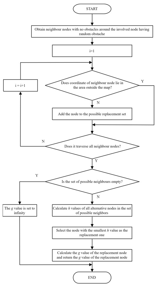
Figure 1. Flowchart of replacement mechanism for the node having random obstacles.

In summary, the proposed replacement strategy introduces a random obstacle replacement mechanism to address the interference with node cost calculations caused by random obstacles, thereby ensuring the continuity and stability of path planning.

3. Detailed Steps of Improved A* Algorithm for Multi-Map Path Planning of Rescuing Robots

The proposed improved A* algorithm for multi-map optimal path planning of rescuing robots follows a systematic workflow, which is visually represented in the flowchart of Figure 2.

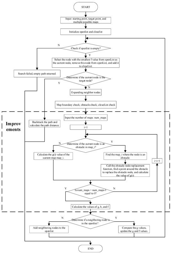
Figure 2. Flowchart of Improved A* for Multi-Map Robot Path Planning.

The flowchart illustrates the algorithm’s iterative execution process, with a prominent “Improvements” segment emphasizing two pivotal innovations: (1) cyclic traversal of multiple environment maps to calculate probabilistically weighted expected costs, and (2) a dedicated obstacle node replacement mechanism for addressing random obstacles. It details the process from inputting start/target points and multi-maps, through node selection and expansion, to dynamic cost updating and path backtracking, ensuring reliable performance in dynamic and uncertain rescue scenarios.

4. Case Study

The proposed improved A* algorithm for multi-map based optimal path planning problem of rescuing robots is implemented in Matlab R2022b programming environment on a desktop computer (CPU i7 3.8 Ghz/16 G RAM) with Windows 10 operating system installed. We consider multiple weighted static maps, whose combination provides a diverse and uncertain environment. However, it is impossible to predict which map will ultimately become the actual environment. Therefore, obstacles in the maps are divided into two categories, fixed obstacles and random obstacles. Fixed obstacles are those that have been identified and exist, and the robot cannot pass through these areas in any map. Conversely, random obstacles are those that have not yet been identified. They may be empty spaces in some maps, but appear as obstacles in others. These obstacles allow the robot passage in some maps, but require adjustment based on the specific circumstances in the actual map. First, the feasibility of the proposed improved A* algorithm is verified by observing whether the obtained planned paths pass through fixed obstacles. Then, the accuracy and optimality of the proposed improved A* algorithm are demonstrated by comparing the path results of the improved A* algorithm and the original algorithm in each possible map. Finally, the stability of the proposed improved A* algorithm is verified through larger-scale and more diverse rescue scenarios.

To more clearly define the core concepts in the following experiments and avoid ambiguity, the paths involved in the research and their specific definitions are systematically sorted out and presented, as shown in Table 1.

Table 1. Path definition in multi-map rescue robot path planning.

Path Name	Path Definition
planning_path	Improved algorithm for generating planning paths
obs_path	Obstacle avoidance paths are generated on each map based on the planned path.
opt_path	Optimal path on each map
map1_planning_path	The traditional A* algorithm plans paths based on map 1.
map2_planning_path	The traditional A* algorithm plans paths based on map 2.
map3_planning_path	The traditional A* algorithm plans paths based on map 3.
map1_obs_path	Obstacle avoidance paths generated for each map based on map1_planning_path
map2_obs_path	Obstacle avoidance paths generated for each map based on map2_planning_path
map3_obs_path	Obstacle avoidance paths generated for each map based on map3_planning_path

4.1. Test Rescuing Scenario

Assume a rescue scenario modeled as a 50 × 50 grid map, where each grid cell measures 1 × 1 m. The map includes both fixed and random obstacles, the latter stemming from limitations of the detection equipment. Based on prior knowledge and expert evaluation, three different grid maps, as shown in Figure 3, were generated and assigned subjective probabilities of 0.4, 0.3, and 0.3, respectively. In the figure, black grids represent fixed obstacles, gray grids represent random obstacles, and white grids represent open areas. The origin of the coordinate system is established in the upper left corner of the grid map, and its horizontal and vertical coordinates represent the column number and row number of the grid. Here in this test scenario, the starting point coordinate of the rescue is (45, 5) and the end point coordinate is (6, 49). Therefore, path planning for rescue robots in a multi-map environment involves finding the optimal path from the starting point to the destination, which minimizes the distance and, by combining obstacle distribution information from each map, avoids all possible fixed obstacles and minimizes the cost of avoiding random obstacles.

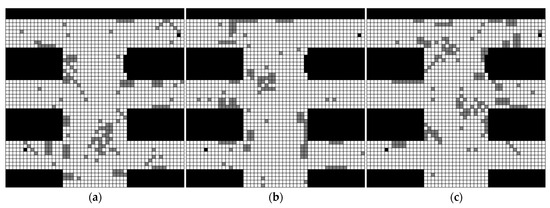
Figure 3. Three distinct grid maps: (a) grid map 1 with subjective probability of 0.4; (b) grid map 2 with subjective probability of 0.3; (c) grid map 3 with subjective probability of 0.3.

4.2. Feasible Analysis of Obtained Planning Paths

The improved A* algorithm generates optimal paths that maintain low obstacle avoidance costs on any map in multiple atlases, thereby ensuring the stability of the path in uncertain environments.

The obtained planning path by the improved A* algorithm is shown in Figure 4. In this figure, all uncertain obstacles are integrated into this map and colored in gray, and red dots indicate the start points while blue dots indicate the target points. It should be noted here that this same color convention is applied in subsequent figures. It is also seen from this figure that there really exists a feasible path which can avoid all possible obstacles from the starting point to the ending point. But why not simply choose this path? That is because the obtained planning path is not the real walking path of the rescuing robots actually. While navigating the planned path generated by the improved A* algorithm, the rescue robot must adjust its actual path based on the obstacles it encounters. As mentioned earlier, this paper utilizes three different grid maps provided by experts to represent the possible obstacle distributions. Therefore, the rescue robot must adopt different obstacle avoidance paths when encountering each scenario map. It should be noted that the traditional A* algorithm is employed here for local obstacle avoidance, that is, when the planning path collides with an obstacle in a certain map scenario, the previous open space node of the collision node in the path is taken as the starting point of the involved collision path, and the first open space node after the path collision node is found as the end point of the involved collision path. The traditional A* algorithm is used to generate a new path to replace the involved collision path in the original planning path. Three adjusted obstacle-avoiding paths (denoted as obs_path) for all possible grid maps as well as the original planning path (denoted as planning_path) are illustrated in Figure 5.

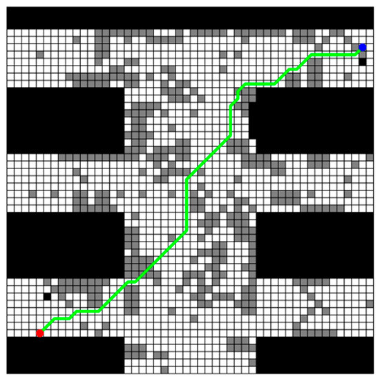
Figure 4. Planning_path generated by improved A* algorithm in multi-map rescuing scenario.

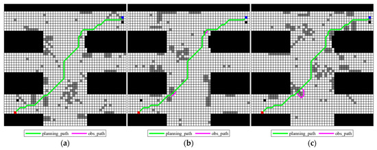
Figure 5. Obs_paths for different possible grid maps: (a) grid map 1; (b) grid map 2; (c) grid map 3.

It can be seen from the obs_path in Figure 5a that the planning_path does not need to be processed for obstacle avoidance in grid map 1. From Figure 5b, it can be seen that in grid map 2, only a small range of obstacle avoidance is performed in the lower left and upper right parts of the path, which has no obvious impact on the path as a whole. For the third possible map in Figure 5c, only one obstacle avoidance is performed in the lower left part. Therefore, by comparing the planning_path and the adjusted ones in Figure 5a–c, it can be found that the planning_path is only adjusted in relatively small times in each map, indicating that the improved algorithm effectively avoids most obstacles and the path planning also well integrates the obstacle information of each map.

For each possible map in the multi-map dataset, the optimal path in each grid map can be obtained using the traditional A* algorithm. Figure 6 shows the adjusted paths on different grid maps and the optimal path (denoted as opt_path) for each deterministic map, clearly demonstrating how close the adjusted paths are to the optimal path of the current map. It can be observed from Figure 6 that although the nodes of the two paths are selected differently, the obs_paths generated by the obtained planning_paths through obstacle-avoiding strategy can closely follow the trend of the opt_paths in terms of bypassing obstacles and choosing the direction of travel. These two paths have significant consistency in characteristics such as the curvature of the path and the location of turning points, indicating that the obs_paths, generated by the proposed improved A* algorithm, are close to the opt_paths in terms of path quality, reflecting good path planning performances. In order to measure how close, the obtained obs_paths are to the opt_path, a closeness function shown in Formula (7) is employed, and the smaller values of the closeness function, the more it can identify the superiority of the obtained planning_path.

$$C_i=L_i\left(P_i^{obs}\right)-L_i\left(P_i^{prophet}\right)$$

(7)

where the $C_i$ estimates the closeness function between the obs_path of the obtained planning_path and the opt_path in the i-th grid map, $L_i\left(x\right)$ is the length calculating function for i-th grid map, and $P_i^{obs}\mathrm{and}{P}_i^{prophet}$ denote the obtained obs_path and the opt_path in the i-th grid map, respectively. Additionally, the closeness percent of length of the obs_path to the opt_path formulated as $\left(1-C_i/L_i\left(P_i^{prophet}\right)\right)\times 100\%$ is also employed to evaluate the performance of the proposed approach. The closeness evaluating results of obs_paths and the opt_paths are shown in Table 2.

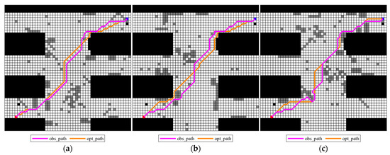
Figure 6. Obs_paths of different possible maps and the opt_paths for each deterministic grid map: (a) grid map 1; (b) grid map 2; (c) grid map 3.

Table 2. Closeness of the obtained obs_paths and the opt_paths in different maps.

Grid Maps	${\mathit{L}}_{\mathit{i}}({\mathit{P}}_{\mathit{i}}^{\mathit{o}\mathit{b}\mathit{s}})$/m	${\mathit{L}}_{\mathit{i}}({\mathit{P}}_{\mathit{i}}^{\mathit{p}\mathit{r}\mathit{o}\mathit{p}\mathit{h}\mathit{e}\mathit{t}})$/m	${\mathit{C}}_{\mathit{i}}$/m	Closeness Percent
map 1	67.1838	65.4264	1.7574	97.31%
map 2	67.7696	64.8406	2.9290	95.48%
map 3	72.0122	69.5269	2.4853	96.43%

As shown in Table 2, the closeness difference in distance of the obs_path and the opt_path in the three maps is between 1.7574 and 2.9290 m, with an overall fluctuation range of 1.3 m, which is relatively small. This shows that the generation of the planning_path fully combines the information of different maps, can stably control the obstacle avoidance cost, and will not cause drastic fluctuations in path length due to scene changes.

To overcome the limitations of the experiment with a single start-end point setting (45, 5) and end-end point (6, 49), an additional experiment was designed with a new start-end point setting (45, 49) and end-end point setting (5, 5) to verify the adaptability and robustness of the improved A* algorithm under different start-end point and end-end point settings. The core variable of this extended experiment is the spatial location of the start-end point; all other experimental conditions remain consistent: the map environment uses the obstacle distribution and size parameters of map 1, map 2, and map 3 and key parameters such as the heuristic function weights and obstacle avoidance handling of the improved algorithm are not adjusted to ensure the comparability and validity of the experimental results. The experimental results are shown in Figure 7 (planning_path generated by the improved A* algorithm), Figure 8 (obs_path and opt_path comparison), and Figure 9 (obs_path and opt_path comparison).

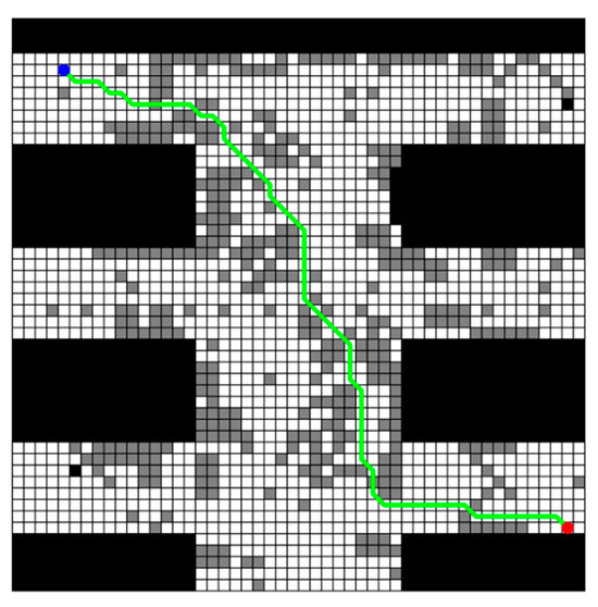
Figure 7. Planning_path generated by an improved A* algorithm with modified origin and destination.

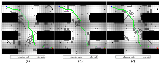
Figure 8. Obs_paths generated with modified origin and destination. (a) Grid map 1; (b) Grid map 2; (c) Grid map 3.

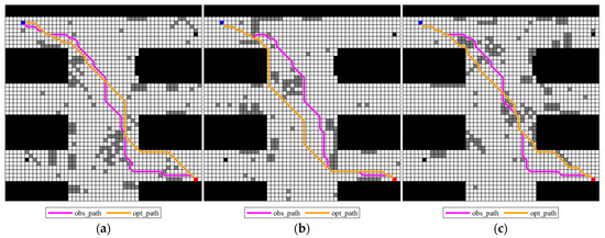
Figure 9. Obs_paths for different possible maps and opt_paths generated for each deterministic grid map with modified origin and destination. (a) Grid map 1; (b) Grid map 2; (c) Grid map 3.

As presented in Figure 7, Figure 8 and Figure 9, the improved A* algorithm can successfully generate reasonable planning_path and obs_path, under the new start-end setting, showing consistent performance in path planning quality without notable fluctuations. Similarly, Formula (7) is used to measure the similarity between obs_path and opt_path, and the results are shown in Table 3.

Table 3. Closeness of the obtained obs_paths and the opt_paths in different maps with modified origin and destination.

Grid Maps	${\mathit{L}}_{\mathit{i}}({\mathit{P}}_{\mathit{i}}^{\mathit{o}\mathit{b}\mathit{s}})$/m	${\mathit{L}}_{\mathit{i}}({\mathit{P}}_{\mathit{i}}^{\mathit{p}\mathit{r}\mathit{o}\mathit{p}\mathit{h}\mathit{e}\mathit{t}})$/m	${\mathit{C}}_{\mathit{i}}$/m	Closeness Percent
map 1	72.5269	66.4264	6.1005	91.59%
map 2	72.5269	69.3553	3.1716	95.63%
map 3	71.6985	65.2548	6.4437	91.01%

As presented in Table 3, under the configuration of modified origin and destination, the Closeness Percent between the obtained obs_paths and opt_paths in map 1, map 2, and map 3 achieves 91.59%, 95.63%, and 91.01%, respectively, all remaining at a relatively high level. This demonstrates that the improved A* algorithm can still maintain a high degree of closeness between obs_paths and opt_paths across different grid maps even with altered start-end points, thus verifying its robust adaptability to start-end configuration changes and the stability of its path planning quality.

4.3. Analysis of Penalty Substitution Strategy

The results above show that the improved A* algorithm can generate planning_path and obs_path that are highly consistent with the opt_path across the three candidate maps. However, a key design consideration is whether the planner should deliberately avoid all random obstacles. To quantitatively examine the trade-off between “complete avoidance” and “allowing moderate traversal,” we introduce a penalty substitution strategy into the random obstacle substitution mechanism, namely, the g value used to replace a random obstacle node is multiplied by a penalty factor $\gamma$, thereby controlling the planner’s tendency to traverse random obstacles. Two controlled experiments with $\gamma =1.2$ and $\gamma =1.4$ are presented below to illustrate how the planner’s performance across different candidate maps changes when forced to avoid random obstacles, and to discuss its balance and conservatism.

When the penalty factor $\gamma =1.2$, the generated planning_path is shown in Figure 10. In each map, the comparison between the obs_paths obtained after obstacle avoidance correction and the corresponding opt_path is shown in Figure 11.

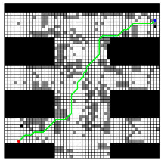
Figure 10. Planning_path under penalty factor $\gamma =1.2$.

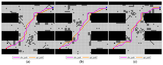
Figure 11. Obs_paths of different possible maps and the opt_paths for each deterministic grid map ($\gamma =1.2$) (a) grid map 1; (b) grid map 2; (c) grid map 3.

It is clearly found from Figure 11 that the three submaps exhibit distinctly different behaviors when $\gamma =1.2$. In maps 1 and 2, the planning_path completely avoids random obstacles, resulting in significant local detours. In map 3, however, the planning_path still traverses some random obstacles, and the obs_path deviates only slightly from the opt_path. This is because the random obstacles in map 3 are primarily located at the edges of the optimal path, and local replacements do not cause significant deviations. Therefore, with $\gamma =1.2$, local replacements in map_3 incur a low cost, preserving good directional consistency. Overall, $\gamma =1.2$ makes the path more conservative, but still maintains some flexibility in certain map structures.

When the penalty factor is increased to 1.4, the planning_path is shown in Figure 12, the comparison between the obs_path and the opt_path in the three maps is shown in Figure 13. It can be observed that as the penalty factor increases beyond a certain threshold, the planning path almost entirely avoids random obstacles, resulting in the obstacle-avoiding path (obs_path) becoming identical across all maps. This not only increases the overall path cost but also causes the obstacle-avoiding path to diverge further from the optimal path (opt_path) of the current map. Therefore, setting the penalty factor too high increases the path’s conservatism, while reducing its flexibility.

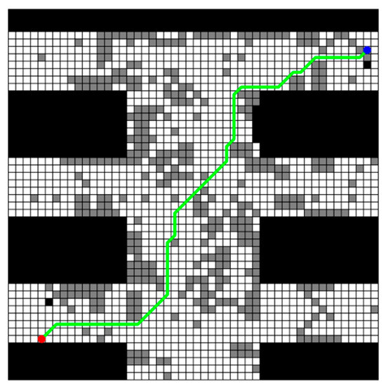
Figure 12. Planning_path under penalty factor $\gamma =1.4$.

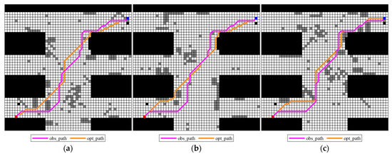
Figure 13. Obs_paths of different possible maps and the opt_paths for each deterministic grid map ($\gamma =1.4$): (a) grid map 1; (b) grid map 2; (c) grid map 3.

Table 4 shows that as the penalty factor $\gamma$ increases, the average closeness decreases continuously, from 96.41% with no penalty to 95.65% with $\gamma =1.2$ and further to 94.20% with $\gamma =1.4$. This indicates that stronger penalty factors cause planned paths to deviate from the oracle optimality overall, resulting in decreased path efficiency. Furthermore, the standard deviation increases from 0.75% to 1.70% and 2.95%, indicating increasing performance imbalance across maps. While paths are more conservative when $\gamma =1.2$, they still maintain good consistency across maps. However, when $\gamma$ increases to 1.4, the average closeness decreases significantly, and the standard deviation nearly doubles, indicating that excessively strong penalties can exacerbate cross-scene disparity. This is due to the uneven distribution of random obstacles across maps. Strong penalties trigger large detours in some maps while having limited impact in others, magnifying the performance gap.

Table 4. Aggregate comparison of penalty factors on the closeness of three candidate maps.

$\mathit{\gamma }$	Map 1	Map 2	Map 3	Mean	Stdv
1.0	97.31%	95.48%	96.43%	96.41%	0.75%
1.2	94.90%	94.05%	98.01%	95.65%	1.70%
1.4	92.54%	91.71%	98.34%	94.20%	2.95%

Overall, the penalty factor can improve conservatism and safety in single-map scenarios, but excessively large values can weaken balance and overall efficiency in multi-map scenarios. Therefore, in missions with multiple candidate maps, a penalty factor of 1.0 should be prioritized.

4.4. Algorithm Performance Comparison

In multi-map robot rescue scenarios, each map may actually occur in the future. Traditionally, the conventional A* algorithm is used to generate a planning path based on a specific scene map, then proceed along that path, adjusting as needed when encountering random obstacles. In this subsection, the path cost results obtained by the proposed improved A* algorithm and the traditional scheme are all reported. Here taking the obtained planning_path by traditional scheme according to grid map 1 as map1_planning_path, and its adjusted path when some certain scenario map happens is denoted as map1_obs_path. So, the planning_path by traditional scheme according to grid map 2 and grid map 3 are named as map2_planning_path and map3_planning_path, and their corresponding adjusted paths are denoted as map2_obs_path and map3_obs_path, respectively. The planning path and the obstacle-avoiding path generated by the proposed improved algorithm are denoted as planning_path and obs_path. The comparisons among the obtained obs_paths by the proposed improved A* algorithm and the traditional one according to grid map 1, grid map 2 and grid map 3 are shown in Figure 14, Figure 15 and Figure 16, and the corresponding path lengths and turning data are listed in Table 5 and Table 6 (for grid map 1), Table 7 and Table 8 (for grid map 2), and Table 9 and Table 10 (for grid map 3), respectively.

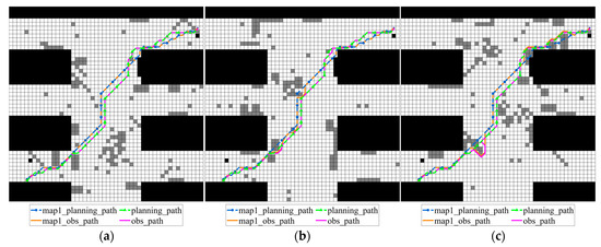
Figure 14. Obs_paths on various possible grid maps obtained by traditional A* algorithm according to grid map 1 and improved A* algorithm: (a) grid map 1; (b) grid map 2; (c) grid map 3.

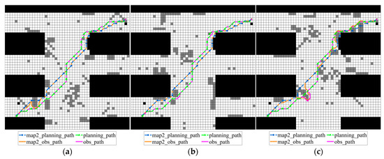
Figure 15. Obs_paths on various possible grid maps obtained by traditional A* algorithm according to map 2 and improved A* algorithm: (a) grid map 1; (b) grid map 2; (c) grid map 3.

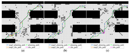
Figure 16. Obs_paths on various possible grid maps obtained by traditional A* algorithm according to map 3 and improved A* algorithm: (a) grid map 1; (b) grid map 2; (c) grid map 3.

Table 5. Length comparisons of the obtained obs_path with map1_obs_path.

Maps	Map Weight	obs_path/m	map1_obs_path/m
map 1	0.4	67.1838	65.4264
map 2	0.3	67.7696	67.5914
map 3	0.3	72.0122	72.4198

Table 6. Comparison of turning performance of various obstacle avoidance paths (obs_path and map1_obs_path) in different map scenarios.

Map	Path	$\mathit{T}$	$\mathit{Z}$	$\mathit{M}$	$\mathit{S}$	$\mathit{C}\mathit{E}\mathit{V}$
map 1	obs_path	18	0	0.0	6	0.0214
	map1_obs_path	18	0	0.0	10	0.1071
map 2	obs_path	19	0	10.3	5	0.1532
	map1_obs_path	28	0	10.7	10	0.6376
map 3	obs_path	23	0	15.5	9	0.3857
	map1_obs_path	23	0	14.6	10	0.3953

Table 7. Length comparisons of the obtained obs_path with map2_obs_path.

Maps	Map Weight	obs_path/m	map2_obs_path/m
map_1	0.4	67.1838	69.8985
map_2	0.3	67.7696	64.8406
map_3	0.3	72.0122	74.4843

Table 8. Comparison of turning performance of various obstacle avoidance paths (obs_path and map2_obs_path) in different map scenarios.

Map	Path	$\mathit{T}$	$\mathit{Z}$	$\mathit{M}$	$\mathit{S}$	$\mathit{C}\mathit{E}\mathit{V}$
map 1	obs_path	18	0	0.0	6	0.0158
	map2_obs_path	29	1	21.5	21	0.8993
map 2	obs_path	19	0	10.3	5	0.1095
	map2_obs_path	22	0	0.0	14	0.1954
map 3	obs_path	23	0	15.5	9	0.2741
	map2_obs_path	33	0	13.3	24	0.6239

Table 9. Length comparisons of the obtained obs_path with map3_obs_path.

Maps	Map Weight	obs_path/m	map3_obs_path/m
map 1	0.4	67.1838	73.2996
map 2	0.3	67.7696	69.5914
map 3	0.3	72.0122	69.5269

Table 10. Comparison of turning performance of various obstacle avoidance paths (obs_path and map3_obs_path) in different map scenarios.

Map	Path	$\mathit{T}$	$\mathit{Z}$	$\mathit{M}$	$\mathit{S}$	$\mathit{C}\mathit{E}\mathit{V}$
map 1	obs_path	18	0	0.0	6	0.0732
	map3_obs_path	31	1	21.7	22	1.0000
map 2	obs_path	19	0	10.3	5	0.1616
	map3_obs_path	17	0	6.1	8	0.1537
map 3	obs_path	23	0	15.5	9	0.3242
	map3_obs_path	13	0	0.0	5	0.0000

In Figure 14, the traditional A* algorithm path map1_planning_path and the improved algorithm generated path planning_path perform obstacle avoidance operations under three different map samples, generating corresponding obstacle avoidance paths map1_obs_path and obs_path. Among them, map1_planning_path is the path generated by the traditional A* algorithm on map_1 and planning_path is the planning_path generated by the improved algorithm proposed in this paper under the consideration of map uncertainty.

From the performance of the obstacle avoidance path, the obs_path generated by the improved algorithm maintains a high degree of consistency under different maps, the path is stable, and the number of turns is small. However, the map1_obs_path formed by the traditional A* path after obstacle avoidance shows obvious deviation and irregular turns, especially when random obstacles appear, it is more likely to have sharp turns or detours. In particular, in Figure 14b, the traditional algorithm path encounters an obstacle in the upper right section and produces a large detour with obvious turns, while the improved algorithm can adjust the path more flexibly and complete obstacle avoidance with only a small change in direction. It can be seen that the improved algorithm is more robust and predictive in dealing with uncertain environments and has higher practical value.

The results in Table 5 show that traditional A* occasionally produces shorter obstacle avoidance paths on certain maps. For example, when the obstacle distributions of map1_planning_path and map_2 perfectly match, the path length is optimal. However, on other maps, significant detours and increased costs often occur. For example, in map 3, the obstacle avoidance path length of the traditional algorithm increases to 72.4198 m, exceeding the 72.0122 m of the improved algorithm, resulting in significant overall fluctuations. In contrast, the improved A* proposed in this paper performs more evenly across the three candidate maps. This demonstrates that by incorporating map uncertainty, the improved algorithm achieves overall robustness and balance across multiple candidate maps, avoiding the significant performance fluctuations often seen with traditional methods across different scenarios.

To further quantify the overall performance of the obstacle avoidance path, a multi-index weighted scoring method was used to quantitatively analyze the path’s turning characteristics. A key step was to address the inconsistency in units among different indicators through normalization. Since indicators such as the number of turns, the number of sharp turns, the standard deviation of angles, and the number of consecutive turns have different dimensions and numerical ranges, direct weighted summation could lead to certain indicators dominating the evaluation value. Normalization employed a min-max scaling method, mapping each indicator to the [0, 1] interval, eliminating the influence of dimensions, and ensuring that all features contribute to the overall evaluation on a fair scale. The evaluation value calculation formula is as follows.

$$CEV={\omega }_1\cdot T^{\prime }+{\omega }_2\cdot Z^{\prime }+{\omega }_3\cdot M^{\prime }+{\omega }_4\cdot S^{\prime }$$

(8)

where $CEV$ denotes the comprehensive evaluation value of the obstacle avoidance path’s turning performance; $T$ represents the number of turns, and its normalized value is denoted as $T^{\prime }$, which reflects the frequency of changes in path direction; $Z$ represents the number of sharp turns (i.e., turning angles greater than 90°), and its normalized value is denoted as $Z^{\prime }$, which measures the severity of sharp turns; $M$ represents the standard deviation of turning angles, and its normalized value is denoted as $M^{\prime }$, which reflects the volatility and consistency of turning angles; $S$ represents the number of consecutive turns, and its normalized value is denoted as $S^{\prime }$, which assesses the density of consecutive direction changes in the path. The weighting coefficients ${\omega }_i$ are set to ${\omega }_1$ = 0.2, ${\omega }_2$ = 0.3, ${\omega }_3$ = 0.2, ${\omega }_4$ = 0.3 to strengthen the penalty for unstable turning behavior. First, the overall path performance of obs_path and map1_obs_path is calculated using Formula (8), and the comparison results are shown in Table 6.

In summary, the quantitative analysis of path length and turning performance shows that the traditional A* algorithm exhibits significant scene dependence and large performance fluctuations in obstacle avoidance path length. The improved A* algorithm, however, not only achieves more balanced path length performance across multiple candidate maps but also demonstrates superior performance compared to the traditional algorithm in dimensions such as the number of turns, the number of sharp turns, the standard deviation of turning angles, the number of consecutive turns, and the overall evaluation value, effectively reducing the instability of path turning. By considering map uncertainty, the improved A* algorithm demonstrates superior overall performance in both obstacle avoidance path length optimization and turning feature stability, exhibiting stronger robustness and practicality.

In Figure 15, the traditional path is generated by the A* algorithm on map_2, denoted as map2_planning_path, and is used as a reference path to perform obstacle avoidance processing under different map samples to generate its corresponding obstacle avoidance path map2_obs_path. Compared with the map1_planning_path path generated based on map_1 in Figure 14, the initial map for generating the traditional path is changed in Figure 15 to verify the impact of different basic paths on the obstacle avoidance results. The path planning_path generated by the improved algorithm and its obstacle avoidance result obs_path remain unchanged as a comparison benchmark.

Comparing map2_obs_path and obs_path, it is found that obs_path has a high proportion of straight segments and fewer turns, which is closer to the shortest path model. As shown in the lower left of Figure 15a, since planning_path takes into account the obstacle distribution of each map when it is generated, obs_path does not need large-angle obstacle avoidance processing, which effectively reduces path redundancy; in the same area, since the generation of map2_planning_path is only related to map_2, and does not take into account the obstacle distribution in map_1, its obstacle avoidance path map2_obs_path has redundant loops and increases the number of turns in the path. As shown in Figure 15c, obs_path only needs to make obstacle avoidance adjustments at a random obstacle in the lower left, and the rest of the time it remains closely aligned with planning_path, reflecting the improved algorithm’s maintenance of the global path direction when avoiding obstacles; while map2_planning_path is significantly separated from map2_obs_path, and map2_obs_path performs multiple obstacle avoidances, resulting in a winding path, reflecting that traditional algorithms find it difficult to maintain the stability of global paths in multiple maps.

In addition, by comparing the path length changes on different maps in Table 7, it can be found that there are obvious differences in path stability. The obstacle avoidance path lengths generated by map2_planning_path range from 64.8406 m to 74.4843 m, with a variation of nearly 10 m. In contrast, the path lengths generated by obs_path of the improved algorithm range from 67.1838 m to 72.0122 m, with a variation in significantly less than 5 m. At the same time, using Formula (9), the sum of the weighted lengths of the obstacle avoidance paths of the improved A* algorithm on the three maps is calculated to be 67.1838 m, while the sum of the weighted lengths of map2_obs_path generated by the traditional A* algorithm is 69.8985 m. This shows that the improved algorithm not only achieves a shorter average weighted path length, but also shows better robustness and consistency in different environments. Therefore, although map2_planning_path performs well in some scenarios, its overall stability is not as good as the improved method.

$$L^w={\displaystyle \sum _{i=1}^n{w}_i}\times L_i\left(x\right)$$

(9)

where $L^w$ is the weighted path length, n is the number of maps, $w_i$ represents the subjective weight of the i-th map, and $L_i\left(x\right)$ represents the obstacle avoidance path length of path x in the i-th grid map.

The path turning performance of obs_path and map2_obs_path was calculated using Formula (8), and the comparison results are shown in Table 8.

By comparing the turning performance evaluation values of different obstacle avoidance paths in Table 8, it can be found that the improved algorithm’s obs_path exhibits better turning behavior stability in all maps, comprehensively outperforming map2_obs_path. In summary, the improved algorithm demonstrates significant advantages in terms of path length scene stability, weighted length optimization effect, and the balance of turning performance, exhibiting stronger robustness and application consistency, and enhancing the reliability of obstacle avoidance path planning in uncertain map environments.

In Figure 16, the traditional path is generated by the A* algorithm on map_3, denoted as map3_planning_path, and obstacle avoidance simulation is performed in multiple different maps to obtain the corresponding map3_obs_path path. The improved path planning_path and its obstacle avoidance result obs_path remain unchanged as a comparison benchmark. As shown in Figure 16a, due to the limitations of the traditional algorithm for multiple maps, the obstacle avoidance path of map3_obs_path deviates significantly from map3_planning_path, forming redundant turns. However, obs_path is close to planning_path and strictly maintains the dominant direction of planning_path, reflecting the improved algorithm’s strong ability to maintain the original planning direction, verifying the improved algorithm’s collaborative optimization of the initial path and obstacle avoidance, reducing invalid turns, and improving path efficiency.

According to the data provided in Table 9, the total weighted obstacle avoidance path length derived from map3_planning_path, calculated using Formula (9), is 71.0553 m, whereas the corresponding value produced by the planning_path of the improved algorithm is 68.8081 m. This indicates that the improved algorithm outperforms the single-map-based map3_planning_path in terms of overall path efficiency. Notably, the longer weighted path length of map3_planning_path is primarily due to suboptimal path performance in map_1 and map_2, where significant detours are observed.

Specifically, in map_1, the obstacle avoidance path length of map3_planning_path reaches 73.2996 m, which is markedly higher than the 67.1838 m generated by the improved algorithm. Similarly, in map_2, a longer path of 69.5914 m is observed, compared to 67.7696 m from the improved method. These results suggest that the path derived from map3_planning_path undergoes multiple obstacle avoidance maneuvers in unfamiliar environments, leading to a more tortuous route. In contrast, the improved algorithm demonstrates stronger adaptability across multiple maps, yielding more consistent and efficient obstacle avoidance paths. Therefore, map3_planning_path shows limited generalization ability and reduced stability in multi-map scenarios.

The path turning performance of obs_path and map3_obs_path was calculated using Formula (8), and the comparison results are shown in Table 10.

As can be seen from Table 10, based on the comprehensive evaluation value of path turning performance, the obs path generated by the improved algorithm exhibits better turning behavior stability in map 1, map 2, and map 3, with the CEV value generally within a reasonable range; while the CEV value of map3_obs_path fluctuates drastically across different maps, indicating limited generalization ability. The improved algorithm demonstrates stronger balance and robustness in turning performance across multiple map scenarios.

The difference between the weighted length of various obstacle avoidance paths and their corresponding planning_path length divided by the planning_path length is recorded as the path redundancy rate shown in Formula (10), which is used to indicate the adaptability of the planning_path to different environmental maps. The smaller the value, the stronger the adaptability to the environment.

$$R={\displaystyle \frac{L^w-L^p}{L^p}}\times 100\%$$

(10)

where R represents the calculated path redundancy rate, which is expressed in percentage; $L^w$ is the sum of weighted obstacle avoidance path lengths; $L^p$ is the corresponding original planning_path length. The path redundancy rate R of planning path (planning_path) by the improved A* algorithm and various planning_paths (map1_planning_path, map2_planning_path and map3_planning_path) by traditional A* algorithm according to different maps are compared and the comparative results are shown in Table 11.

Table 11. Comparison of path redundancy ratio R in multiple schemes.

Baseline Path	Reference Path Length/m	Weighted Sum Length of obs_path/m	Path Redundancy Rate/%
planning_path	67.1838	68.8081	2.4177
map1_planning _path	65.4264	68.1739	4.1994
map2_planning _path	64.8406	69.7569	7.5821
map3_planning _path	69.5269	71.0553	2.1983

As shown in Table 11, the path redundancy rate of the improved algorithm’s planning_path is 2.4177%, significantly lower than the 4.1994% of the map1_planning_path and the 7.5821% of the map2_planning_path. This demonstrates that the paths generated by the improved A* algorithm are more adaptable and consistent across multiple maps. By comprehensively considering information from multiple candidate maps, the improved algorithm effectively avoids generating unnecessary long detours, resulting in lower path redundancy. In contrast, the traditional A* algorithm’s map1_planning_path and map2_planning_path have higher redundancy rates of 4.1994% and 7.5821%, respectively, indicating poor adaptability across different maps. In particular, the high redundancy rate in map_2 reflects the traditional algorithm’s inability to effectively adapt its paths across different maps, resulting in longer detours in new environments. Although the redundancy rate of map3_planning_path is 2.1983%, lower than that of planning_path, its path length is significantly longer, reaching 71.0553 m, compared to 68.8081 m for planning_path. This is clearly demonstrated by comparing the path diagrams in Figure 16. While the redundancy rate of map3_planning_path in map_3 is lower, its generation process based on a single map results in unnecessary detours, increasing the total path length. Therefore, despite the lower redundancy rate of map3_planning_path, its overall path efficiency is significantly lower than that of planning_path. Overall, the planning_path generated by the improved algorithm demonstrates better adaptability, robustness, and path efficiency in a multi-map environment, making it a more preferred choice for obstacle avoidance tasks with multiple candidate maps.

4.5. Large-Scale and Multi-Map Quantity Extended Verification

In order to test the stability of the proposed multi-map rescuing path planning approach, a larger rescuing scenario of 100 × 100 grid map with each grid size of 1 m × 1 m is employed. The scenario is still assumed to have three possible maps with subjective probabilities as 0.4, 0.3 and 0.3. The coordinates of the starting point for this rescuing are (93, 7), and the coordinates of the end point are (12, 98). The planned path generated by the proposed improved A* algorithm, denoted as planning_path, where fixed obstacles are represented in black and uncertain obstacles in gray, is shown in Figure 17. The planning_path and its corresponding obstacle avoidance path for each possible scenario map, denoted as obs_path, and the optimal path under the current map, denoted as opt_path, are shown in Figure 18.

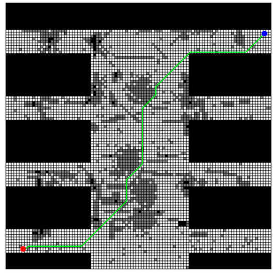
Figure 17. Planning_path generated by improved A* algorithm in multi-map rescuing scenario for 100 × 100 map.

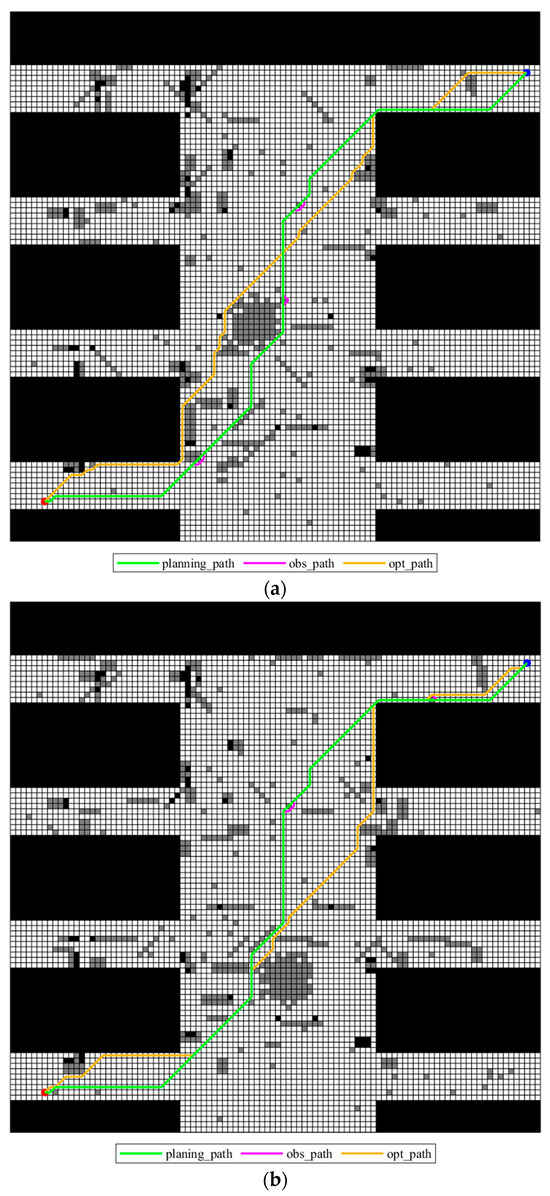
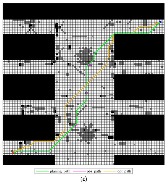
Figure 18. Obs_paths of different possible maps and the opt_paths for each deterministic grid map for 100 × 100 map: (a) grid map 1; (b) grid map 2; (c) grid map 3.

As shown in Figure 18, the planning_path generated by the improved A* algorithm demonstrates strong feasibility and stability across multiple maps. Despite variations in obstacle distribution among the maps, the corresponding obs_path remains largely consistent, with only minor local detours occurring to facilitate obstacle avoidance. In each map, the opt_path is generated by the traditional A* algorithm as the optimal reference path. A careful comparison of the obs_path and opt_path’s closeness across all test maps reveals a similar number of turning points, high synergy in direction, and a near-perfect parallelism between the two paths. This demonstrates that the improved A* algorithm maintains the best possible alignment with the optimal path’s planning logic while meeting obstacle avoidance requirements.

To further verify the stability of the proposed multi-map path planning method in uncertain environments, six map samples were introduced onto the initial 50 × 50 grid map, with weights w = [0.3, 0.25, 0.2, 0.1, 0.1, 0.05]. The starting coordinates were (45.5) and the ending coordinates were (6, 49). Each map contained a different distribution of uncertain obstacles, reflecting the ambiguity and diversity of map perception in typical post-disaster scenarios.

In this experiment, firstly, under multiple maps, a unified planned path, denoted as planning_path, was generated using the improved A* algorithm. Then, obstacle avoidance paths, denoted as obs_paths, were generated on each map separately. Simultaneously, the traditional A* algorithm was used to generate the corresponding optimal path, denoted as opt_path, on each possible map, as a reference. The experimental results are shown in Figure 19 and Figure 20, and the path length and proximity index statistics are shown in Table 12.

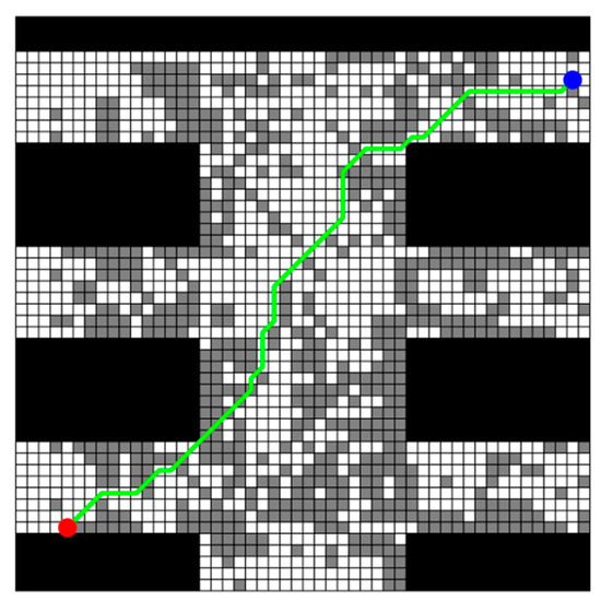
Figure 19. Improved A* algorithm for planning_path generation of six maps in multi-map rescue scenarios.

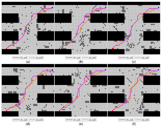
Figure 20. Obstacle avoidance paths for six maps and the best oracle path for each deterministic grid map: (a) Grid Map 1; (b) Grid Map 2; (c) Grid Map 3; (d) Grid Map 4; (e) Grid Map 5; (f) Grid Map 6.

Table 12. The degree of closeness between the obstacle avoidance paths obtained in the six maps and the optimal predicted path.

Grid Maps	${\mathit{L}}_{\mathit{i}}({\mathit{P}}_{\mathit{i}}^{\mathit{o}\mathit{b}\mathit{s}})$/m	${\mathit{L}}_{\mathit{i}}({\mathit{P}}_{\mathit{i}}^{\mathit{p}\mathit{r}\mathit{o}\mathit{p}\mathit{h}\mathit{e}\mathit{t}})$/m	${\mathit{C}}_{\mathit{i}}$/m	Closeness Percent
map 1	66.5980	64.8406	1.7574	97.36%
map 2	67.1838	65.4264	1.7574	97.38%
map 3	68.0122	65.4264	2.5858	96.20%
map 4	70.5980	66.5980	4.0000	94.33%
map 5	67.1838	65.4264	1.7574	97.38%
map 6	68.5980	66.0122	2.5858	96.23%

As can be seen from Table 12, except for map 4, the Closeness Percent of the obstacle avoidance path and the optimal path of the remaining maps is higher than 96%, among which maps 1, 2, and 5 perform particularly well, with a difference in only 1.7574 m. This shows that the global path generated by the improved algorithm has good compatibility in most scenarios and can complete obstacle avoidance with relatively small adjustments, reflecting strong robustness.

5. Conclusions

The improved A* algorithm proposed in this study shows significant advantages in the path planning of rescue robots in multi-environment maps by integrating multi-map weighted mechanism and random obstacle replacement strategy. Experiments show that the improved algorithm is superior to traditional methods in weighted obstacle avoidance path length, path redundancy rate and cross-map stability, providing a more efficient and stable solution for complex rescue scenarios.

(1) By weighted fusion of path costs and heuristic functions of multiple maps, the improved algorithm integrates obstacle distribution and weight information of different maps, effectively reducing the path redundancy rate. Experimental data show that in a 50 × 50 scale map, the path redundancy rate of the baseline path planning_path generated by the improved algorithm is only 2.4177%, which is much lower than 4.1994% of map1_planning_path and 7.5821% of map2_planning_path generated by a single map. It shows that the mechanism can balance path efficiency and obstacle avoidance requirements in a multi-map environment and reduce redundant adjustments.

(2) A local replacement strategy designed for random obstacles ensures path continuity by rapidly selecting adjacent open space nodes to replace obstructed paths. Comparative experiments show that the obstacle avoidance paths generated based on planning_path require only local fine-tuning within each map, resulting in obstacle avoidance costs of only 1.7574, 2.9290, and 2.4853 m, respectively. The weighted total lengths of the obstacle avoidance paths generated based on the single maps map2_planning_path, and map3_planning_path are 69.7569, and 71.0553 m, respectively, all exceeding the 68.8081 m of the improved algorithm. This demonstrates its high tolerance to random obstacles.

(3) In terms of stability verification, in three large-scale 100 × 100 maps with weights of 0.4, 0.3, and 0.3, the obstacle avoidance path of the improved algorithm is highly consistent with the optimal path, and only local fine-tuning is required to complete obstacle avoidance and ensure path continuity. Expanding to six 50 × 50 maps with weights of 0.3, 0.25, 0.2, 0.1, 0.1, and 0.05, except for map 4, where the obstacle avoidance path is 94.33% close to the optimal path, the closeness of the remaining maps exceeds 96%, and the difference in closeness between maps 1, 2, and 5 is only 1.7574 m. It can be seen that the improved algorithm has high stability and strong robustness in complex multi-map scenarios.

The improved A* algorithm achieves the coordinated optimization of path planning efficiency and stability through multi-map information fusion and random obstacle processing mechanism. Its low redundancy rate, low obstacle avoidance cost and consistent performance across scenarios in complex and uncertain environments provide reliable technical support for practical applications such as unmanned driving and post-disaster rescue. In the future, we can further explore dynamic weight adjustment and large-scale map parallel computing to enhance the real-time and scalability of the algorithm.

References

- Bu, X.; Su, H.; Zou, W.; Wang, P.; Zhou, H. Ant colony path planning based on non-uniform modeling of complex environments. Robotics 2016, 38, 276–284. [Google Scholar] [CrossRef]
- Liu, J.; Chen, X.; Xiao, J.; Lin, S.; Zheng, Z.; Lu, H. Hybrid Map-Based Path Planning for Robot Navigation in Unstructured Environments. In Proceedings of the 2023 IEEE/RSJ International Conference on Intelligent Robots and Systems (IROS), Detroit, MI, USA, 13 December 2023; pp. 2216–2223. [Google Scholar] [CrossRef]
- Xie, W.; Fang, X.; Wu, S. 2.5D Navigation Graph and Improved A-Star Algorithm for Path Planning in Ship inside Virtual Environment. In Proceedings of the 2020 Prognostics and Health Management Conference (PHM-Besançon), Besancon, France, 4–7 May 2020; pp. 295–299. [Google Scholar] [CrossRef]
- Li, F.; Kim, Y.-C.; Xu, B. Non-Standard Map Robot Path Planning Approach Based on Ant Colony Algorithms. Sensors 2023, 23, 7502. [Google Scholar] [CrossRef]
- Lee, D.; Nahrendra, I.M.A.; Oh, M.; Yu, B.; Myung, H. TRG-Planner: Traversal Risk Graph-Based Path Planning in Unstructured Environments for Safe and Efficient Navigation. IEEE Robot. Autom. Lett. 2025, 10, 1736–1743. [Google Scholar] [CrossRef]
- Zhao, S.; Hwang, S.-H. Complete coverage path planning scheme for autonomous navigation ROS-based robots. ICT Express 2024, 10, 83–89. [Google Scholar] [CrossRef]
- Lu, J.; Zeng, B.; Tang, J.; Lam, T.L.; Wen, J. TMSTC*: A Path Planning Algorithm for Minimizing Turns in Multi-Robot Coverage. IEEE Robot. Autom. Lett. 2023, 8, 5275–5282. [Google Scholar] [CrossRef]
- Sun, J.; Sun, Z.; Wei, P.; Liu, B.; Wang, Y.; Zhang, T.; Yan, C. Path Planning Algorithm for a Wheel-Legged Robot Based on the Theta* and Timed Elastic Band Algorithms. Symmetry 2023, 15, 1091. [Google Scholar] [CrossRef]
- Mısır, O. Dynamic local path planning method based on neutrosophic set theory for a mobile robot. J. Braz. Soc. Mech. Sci. Eng. 2023, 45, 127. [Google Scholar] [CrossRef]
- Gan, X.; Huo, Z.; Li, W. DP-A*: For Path Planing of UGV and Contactless Delivery. IEEE Trans. Intell. Transp. Syst. 2024, 25, 907–919. [Google Scholar] [CrossRef]
- Luo, M.; Hou, X.; Yang, J. Surface Optimal Path Planning Using an Extended Dijkstra Algorithm. IEEE Access 2020, 8, 147827–147838. [Google Scholar] [CrossRef]
- Lan, W.; Jin, X.; Wang, T.; Zhou, H. Improved RRT Algorithms to Solve Path Planning of Multi-Glider in Time-Varying Ocean Currents. IEEE Access 2021, 9, 158098–158115. [Google Scholar] [CrossRef]
- Wu, Q.; Chen, H.; Liu, B. Path Planning of Agricultural Information Collection Robot Integrating Ant Colony Algorithm and Particle Swarm Algorithm. IEEE Access 2024, 12, 50821–50833. [Google Scholar] [CrossRef]
- Zhang, J.; Xu, Z.; Liu, H.; Zhu, X.; Lan, B. An Improved Hybrid Ant Colony Optimization and Genetic Algorithm for Multi-Map Path Planning of Rescuing Robots in Mine Disaster Scenario. Machines 2025, 13, 474. [Google Scholar] [CrossRef]
- Li, D.; Wang, L.; Cai, J.; Ma, K.; Tan, T. Research on Terminal Distance Index-Based Multi-Step Ant Colony Optimization for Mobile Robot Path Planning. IEEE Trans. Autom. Sci. Eng. 2022, 20, 2321–2337. [Google Scholar] [CrossRef]
- Yu, J.; Su, Y.; Liao, Y. The Path Planning of Mobile Robot by Neural Networks and Hierarchical Reinforcement Learning. Front. Neurorobotics 2020, 14, 63. [Google Scholar] [CrossRef]
- Chen, L.; Wang, Q.; Deng, C.; Xie, B.; Tuo, X.; Jiang, G. Improved Double Deep Q-Network Algorithm Applied to Multi-Dimensional Environment Path Planning of Hexapod Robots. Sensors 2024, 24, 2061. [Google Scholar] [CrossRef]
- Guo, B.; Kuang, Z.; Guan, J.; Hu, M.; Rao, L.; Sun, X. An Improved A-Star Algorithm for Complete Coverage Path Planning of Unmanned Ships. Int. J. Pattern Recognit. Artif. Intell. 2022, 36, 2259009. [Google Scholar] [CrossRef]
- Wang, X.; Ma, X.; Li, Z. Research on SLAM and Path Planning Method of Inspection Robot in Complex Scenarios. Electronics 2023, 12, 2178. [Google Scholar] [CrossRef]
- Huang, S.; Wu, X.; Huang, G. Depth-inspired improved 3D A* algorithm based on dynamic field of view. Robotics 2024, 46, 513–523. [Google Scholar] [CrossRef]
- Huang, C.; Zhao, Y.; Zhang, M.; Yang, H. APSO: An A*-PSO Hybrid Algorithm for Mobile Robot Path Planning. IEEE Access 2023, 11, 43238–43256. [Google Scholar] [CrossRef]
- Zhang, B.; Cai, X.; Li, G.; Li, X.; Peng, M.; Yang, M. A modified A* algorithm for path planning in the radioactive environment of nuclear facilities. Ann. Nucl. Energy 2025, 214, 111233. [Google Scholar] [CrossRef]
- Hu, L.; Wei, C.; Yin, L. Fuzzy A∗ quantum multi-stage Q-learning artificial potential field for path planning of mobile robots. Eng. Appl. Artif. Intell. 2025, 141, 109866. [Google Scholar] [CrossRef]
- Zhen, R.; Gu, Q.; Shi, Z.; Suo, Y. An Improved A-Star Ship Path-Planning Algorithm Considering Current, Water Depth, and Traffic Separation Rules. J. Mar. Sci. Eng. 2023, 11, 1439. [Google Scholar] [CrossRef]
- Qin, H.; Shao, S.; Wang, T.; Yu, X.; Jiang, Y.; Cao, Z. Review of Autonomous Path Planning Algorithms for Mobile Robots. Drones 2023, 7, 211. [Google Scholar] [CrossRef]
- Sun, Y.; Yuan, Q.; Gao, Q.; Xu, L. A Multiple Environment Available Path Planning Based on an Improved A* Algorithm. Int. J. Comput. Intell. Syst. 2024, 17, 172. [Google Scholar] [CrossRef]
- Liu, L.; Wang, B.; Xu, H. Research on Path-Planning Algorithm Integrating Optimization A-Star Algorithm and Artificial Potential Field Method. Electronics 2022, 11, 3660. [Google Scholar] [CrossRef]
- Wang, P.; Mutahira, H.; Kim, J.; Muhammad, M.S. ABA*–Adaptive Bidirectional A* Algorithm for Aerial Robot Path Planning. IEEE Access 2023, 11, 103521–103529. [Google Scholar] [CrossRef]
- Lai, R.; Wu, Z.; Liu, X.; Zeng, N. Fusion Algorithm of the Improved A* Algorithm and Segmented Bézier Curves for the Path Planning of Mobile Robots. Sustainability 2023, 15, 2483. [Google Scholar] [CrossRef]
- Huang, J.; Chen, C.; Shen, J.; Liu, G.; Xu, F. A self-adaptive neighborhood search A-star algorithm for mobile robots global path planning. Comput. Electr. Eng. 2025, 123(Part A), 110018. [Google Scholar] [CrossRef]
Disclaimer/Publisher’s Note: The statements, opinions and data contained in all publications are solely those of the individual author(s) and contributor(s) and not of MDPI and/or the editor(s). MDPI and/or the editor(s) disclaim responsibility for any injury to people or property resulting from any ideas, methods, instructions or products referred to in the content. |
© 2025 by the authors. Licensee MDPI, Basel, Switzerland. This article is an open access article distributed under the terms and conditions of the Creative Commons Attribution (CC BY) license (https://creativecommons.org/licenses/by/4.0/).