Parameter Identification in FEM of Mechanical Structure Within NPP Based on Seismic Response

Abstract

Reliable finite element models (FEMs) are required in seismic qualification of mechanical structures within a nuclear power plant (NPP). The relative displacement response of such mechanical structures is difficult to measure, and it is costly to extract enough modes. Therefore, the modification of the initial FEM by the common FEM updating method could not always be carried out smoothly. In this paper, a vibration control equation error-based two-stage FEM updating method is proposed to identify uncertain parameters in the FEMs, which is capable of employing seismic response in the form of acceleration. Optimal values of updating parameters are searched by using the Marquardt method, which is effective in avoiding the ill-conditioned iterative equation. Numerical simulation is performed for the steam pipeline to validate the actual feasibility and robustness of the proposed method. The fact that the distribution of damping is independent of the identification of parameters related to the mass and stiffness matrices is also demonstrated. Finally, experimental validation of the method is carried out on a load-bearing pipeline. The damping coefficients of the pipeline are modified independently by back propagation neural network.

1. Introduction

Seismic response prediction provides the essential data foundation for the equipment qualification, seismic margin assessment [1,2]. The seismic response prediction by the shaking table testing generally has some limitations, which are due to the possibility for the size and load capacity of the table to restrict testing of large structures or the difficulty for boundary conditions to reflect in the test. Moreover, the configuration, mass, and stiffness of the structural are possible to change over time due to either addition or removal of some components, which makes the experiments unable to be performed again after installation in general. Therefore, the FE method is regarded as the most commonly used approach to the seismic response prediction of mechanical structures within NPP [3]. In spite of this, the existing FE method remains incapable of providing sufficiently accurate FEMs, especially in the field of dynamics. Model updating as an effective way of reducing the inaccuracies present in FEMs using experimental data is widely applied [4]. To improve the predictive accuracy for seismic response, Sinha et al. [5,6] employed an eigensensitivity-based iterative method to update the FEM of nuclear-grade piping. However, mechanical structures within NPPs often face the challenge of having an insufficient number of experimentally identified modes. This precludes the establishment of a mathematical model with a unique solution. As a solution, Kim et al. [7], Park et al. [8] manually updated the initial FEMs of concrete containments to make the theoretical modes consistent with the measured modes.

In conclusion, the eigensensitivity-based model updating method can improve the reliability of static or dynamic analysis results. Yet, the accuracy of modal extraction determines how reliable the updated model is. In general, especially for mechanical structures, modes are unlikely to be identified accurately and in sufficient numbers. The eigensensitivity-based iterative method is also weak in identifying the damping matrix. In order to make up for the defect of eigensensitivity-based methods and provide a simple way to identify damping matrix, Chen et al. [9] raised a frequency response function (FRF) error-based model updating method. However, the inherent complexity associated with FRF limits its practical application. To remove the potential need of modal tests or FRF measurements, Zhao and Yu [10] suggested the model updating method that is capable of incorporating base excitation test data directly. For the mechanical structures within NPPs, the readily available vibration test data are the seismic responses in the form of acceleration detected during service or simulated operation tests, which are typical responses under basic excitation. However, it is impractical to attempt to update the FEMs of such structures using the method proposed by Lin and Zhu [11], because the derivation process of the method assumed that both the input and output of the basic excitation are displacements and that only the fixed nodes are loaded.

In the field of bridge engineering, there are plenty of examples of using the acceleration response monitored from the ambient vibration test to complete the identification of uncertain parameters of the bridge FEM [12,13,14,15]. Unfortunately, the actual test data used in the identification process are still the modes extracted from these acceleration responses. The long span of the bridge ensures that a sufficient number of modes can be extracted from the ambient vibration data, whereas the seismic response of nuclear power equipment usually contains only a small number of modes, or even only the fundamental frequency. Fu and Wang [16] directly defined the error between the measured response and the simulated response in the time domain and searched for the optimal solution of uncertain parameters through the adaptive algorithm. Nevertheless, due to the complexity of the calculation process, it was not widely used in practice. In summary, the wide array of existing model updating methods are largely unsuitable for NPP applications. Consequently, a model updating method that leverages readily obtainable vibration data is urgently required to improve the reliability of FE predictions for both dynamic and static responses of NPP mechanical structures.

In this paper, a vibration control equation error (VCEE)-based two-stage FEM updating is suggested, which has the capability to identify uncertain parameters by utilizing seismic response straightaway. The damping coefficients are modified independently by back propagation neural network (BPNN) in stage II. The effectiveness and robustness are validated with several computational cases on a steam pipeline. The treatment of damping and imaginary parts and the principle of frequency selection in the uncertain parameter identification process are studied and discussed. Subsequently, a shaking table test was performed on a pipeline. The method is used to identify the uncertain parameters in the FEM of the pipeline.

2. Model Updating Theory Derivation

For the structure subjected to earthquake excitation, the vibration control equation of the system in frequency domain can be expressed as:

$$(\mathbf{M}+\mathrm{i}{\omega }^{-1}\mathbf{C}-{\omega }^{-2}\mathbf{K})\ddot{\mathbf{u}}=\mathbf{-}\mathbf{M}{\ddot{\mathbf{u}}}_{\mathrm{g}}$$

(1)

where M, C, K, denote the mass matrix, the viscous damping matrix, and the stiffness matrix, respectively. $\ddot{\mathbf{u}}$ and ${\ddot{\mathbf{u}}}_{\mathbf{g}}$ represent the relative acceleration response vector and the seismic excitation vector in frequency domain, respectively. Equation (1) can be abbreviated as:

$$\mathbf{B}\ddot{\mathbf{u}}=-\mathbf{M}{\ddot{\mathbf{u}}}_{\mathrm{g}}$$

(2)

B indicates dynamic stiffness matrix. Equation (2) can be understood as the balance of forces for the structure at the time of earthquake. The VCEE is written as:

$$\mathbf{\epsilon }=-\mathbf{M}{\ddot{\mathbf{u}}}_{\mathrm{g}}-\mathbf{B}\ddot{\mathbf{u}}$$

(3)

Considering that B representing the initial FEM deviates from the practical structure, the ε on the left side of Equation (3) is generally not equal to zero. Suppose θ = {θ₁, θ₂, θ₃…θ_p}^T is the vector of updating parameters in association with FEM physical variables. M and B are represented by the Taylor series expansion of updating parameters with nonlinear terms discarded. Then, Equation (3) has the following form:

$$\mathbf{\epsilon }=-{\mathbf{M}}_0{\ddot{\mathbf{u}}}_{\mathrm{g}}-{\mathbf{B}}_0\ddot{\mathbf{u}}-{\displaystyle \frac{\partial (\mathbf{M}{\ddot{\mathbf{u}}}_{\mathrm{g}}+\mathbf{B}\ddot{\mathbf{u}})}{\partial \mathbf{\theta }}}\mathrm{d}\mathbf{\theta }$$

(4)

Equation (4) can be abbreviated as:

$$\mathbf{\epsilon }=\mathbf{b}-\mathbf{A}\mathrm{d}\mathbf{\theta }$$

(5)

A is the sensitivity matrix of updating parameters to VCEE. ω = {ω₁, ω₂, ω₃…ω_q }^T is the frequency vector participating in the updating process. b, dθ, and A show the following forms:

$$\mathbf{b}={\left\{\begin{array}{c}-{\mathbf{M}}_0{\ddot{\mathbf{u}}}_{\mathrm{g}}({\omega }_1)-{\mathbf{B}}_0\ddot{\mathbf{u}}({\omega }_1)\\ -{\mathbf{M}}_0{\ddot{\mathbf{u}}}_{\mathrm{g}}({\omega }_2)-{\mathbf{B}}_0\ddot{\mathbf{u}}({\omega }_2)\\ ⋮\\ -{\mathbf{M}}_0{\ddot{\mathbf{u}}}_{\mathrm{g}}({\omega }_{\mathrm{q}})-{\mathbf{B}}_0\ddot{\mathbf{u}}({\omega }_{\mathrm{q}})\end{array}\right\}}_{(\mathrm{q}\times \mathrm{n})\times 1}$$

(6)

$$\left\{\mathrm{d}\theta \right\}={\left\{\begin{array}{c}\mathrm{d}{\theta }_1\\ \mathrm{d}{\theta }_2\\ ⋮\\ \mathrm{d}{\theta }_{\mathrm{p}}\end{array}\right\}}_{\mathrm{p}\times 1}$$

(7)

$$\mathrm{A}={\left[\begin{array}{cccc}{\displaystyle \frac{\partial \mathbf{M}}{\partial {\theta }_1}}{\ddot{\mathbf{u}}}_{\mathrm{g}}({\omega }_1)+{\displaystyle \frac{\partial \mathbf{B}}{\partial {\theta }_1}}\ddot{\mathbf{u}}({\omega }_1)& {\displaystyle \frac{\partial \mathbf{M}}{\partial {\theta }_2}}{\ddot{\mathbf{u}}}_{\mathrm{g}}({\omega }_1)+{\displaystyle \frac{\partial \mathbf{B}}{\partial {\theta }_2}}\ddot{\mathbf{u}}({\omega }_1)& \dots & {\displaystyle \frac{\partial \mathbf{M}}{\partial {\theta }_p}}{\ddot{\mathbf{u}}}_{\mathrm{g}}({\omega }_1)+{\displaystyle \frac{\partial \mathbf{B}}{\partial {\theta }_{\mathrm{p}}}}\ddot{\mathbf{u}}({\omega }_1)\\ {\displaystyle \frac{\partial \mathbf{M}}{\partial {\theta }_1}}{\ddot{\mathbf{u}}}_{\mathrm{g}}({\omega }_2)+{\displaystyle \frac{\partial \mathbf{B}}{\partial {\theta }_1}}\ddot{\mathbf{u}}({\omega }_2)& {\displaystyle \frac{\partial \mathbf{M}}{\partial {\theta }_2}}{\ddot{\mathbf{u}}}_{\mathrm{g}}({\omega }_2)+{\displaystyle \frac{\partial \mathbf{B}}{\partial {\theta }_2}}\ddot{\mathbf{u}}({\omega }_2)& \dots & {\displaystyle \frac{\partial \mathbf{M}}{\partial {\theta }_{\mathrm{p}}}}{\ddot{\mathbf{u}}}_{\mathrm{g}}({\omega }_2)+{\displaystyle \frac{\partial \mathrm{B}}{\partial {\theta }_{\mathrm{p}}}}\ddot{\mathbf{u}}({\omega }_2)\\ ⋮& ⋮& \dots & ⋮\\ {\displaystyle \frac{\partial \mathbf{M}}{\partial {\theta }_1}}{\ddot{\mathbf{u}}}_{\mathrm{g}}({\omega }_{\mathrm{q}})+{\displaystyle \frac{\partial \mathbf{B}}{\partial {\theta }_1}}\ddot{\mathbf{u}}({\omega }_{\mathrm{q}})& {\displaystyle \frac{\partial \mathbf{M}}{\partial {\theta }_2}}{\ddot{\mathbf{u}}}_{\mathrm{g}}({\omega }_{\mathrm{q}})+{\displaystyle \frac{\partial \mathbf{B}}{\partial {\theta }_2}}\ddot{\mathbf{u}}({\omega }_{\mathrm{q}})& \dots & {\displaystyle \frac{\partial \mathbf{M}}{\partial {\theta }_{\mathrm{p}}}}{\ddot{\mathbf{u}}}_{\mathrm{g}}({\omega }_{\mathrm{q}})+{\displaystyle \frac{\partial \mathbf{B}}{\partial {\theta }_{\mathrm{p}}}}\ddot{\mathbf{u}}({\omega }_{\mathrm{q}})\end{array}\right]}_{(\mathrm{q}\times \mathrm{n})\times \mathrm{p}}$$

(8)

The subscripts p, q, and n represent the number of updating parameters, the selected frequency points, and the degree of freedoms, respectively. If the acceleration measurement data of sufficient frequency is used (q > p), Equation (5), which indicates the basic equation of the approach proposed in this paper to updating FEM, can be converted into a set of over-determined algebraic equations.

A higher quality FEM is constructed by searching a parameter vector θ that minimizes ε. Constructing the penalty function for ε. To prevent unreasonable changes in the updating parameters, a weighted matrix and the initial estimation information on the updating parameters are introduced in the penalty function:

$$\mathrm{J}(\mathrm{d}\mathbf{\theta })={\Vert \mathbf{\epsilon }\Vert }^2={(\mathbf{b}-\mathbf{A}\mathrm{d}\mathbf{\theta })}^{\mathrm{T}}(\mathbf{b}-\mathbf{A}\mathrm{d}\mathbf{\theta })+{(\mathbf{\theta }-{\mathbf{\theta }}_0)}^{\mathrm{T}}\mathbf{W}(\mathbf{\theta }\mathbf{-}{\mathbf{\theta }}_0)$$

(9)

W and θ₀ denote weighted matrix and initial estimation of the parameter, respectively. Due to only linear terms being retained, the optimal updating parameter value needs to be calculated in iteration. The partial differential of J(dθ) assigned to dθ equals zero; meanwhile, making dθ = θ_i+1 − θ_i, an iterative mathematical formula for FEM updating can be expressed as:

$${\mathbf{\theta }}_{\mathrm{i}+1}={\mathbf{\theta }}_{\mathrm{i}}+{\left[{\mathbf{A}}^{\mathrm{T}}\mathbf{A}+\mathbf{W}\right]}^{-1}({\mathbf{A}}^{\mathrm{T}}\mathbf{b}-\mathbf{W}({\mathbf{\theta }}_{\mathrm{i}}-{\mathbf{\theta }}_0))$$

(10)

where θ_i, and the subscript i represent current estimate of the parameter and iteration step, respectively. During the execution of the strategy, it is desirable to assign smaller weights to more uncertain parameters to mitigate its magnitude of change, hence the inverse of the covariance matrix of the updated parameter matrix is selected as the weighting matrix. W is shown in Equation (11). θ_pi represents the value of the p-th parameter in the i-th iteration.

$$\mathbf{W}={\left\{\mathrm{COV}\left(\left[\begin{array}{cccc}\begin{array}{c}{\theta }_{11}\\ {\theta }_{12}\\ ⋮\\ {\theta }_{1\mathrm{i}}\end{array}& \begin{array}{c}{\theta }_{21}\\ {\theta }_{22}\\ ⋮\\ {\theta }_{2\mathrm{i}}\end{array}& \begin{array}{c}\dots \\ \dots \\ \dots \\ \dots \end{array}& \begin{array}{c}{\theta }_{\mathrm{p}1}\\ {\theta }_{\mathrm{p}2}\\ ⋮\\ {\theta }_{\mathrm{p}\mathrm{i}}\end{array}\end{array}\right]\right)\right\}}^{-1}$$

(11)

If [A^TA] is singular or close to singular, solving Equation (10) by least squares method may result in a set of parameters that violate objective practice and have the potential to reduce the input residual. In order to change the eigenvalue structure of the original matrix, an effective method is to add a positive definite diagonal matrix to [A^TA] for the sake of making it a positive definite matrix with better condition numbers. This is known as the Marquardt algorithm. Equation (10) can be expressed as:

$${\mathbf{\theta }}_{\mathrm{i}+1}={\mathbf{\theta }}_{\mathrm{i}}+{\left[{\mathbf{A}}^{\mathrm{T}}\mathbf{A}+\mathbf{W}+\lambda \mathbf{I}\right]}^{-1}({\mathbf{A}}^{\mathrm{T}}\mathbf{b}-\mathbf{W}({\mathbf{\theta }}_{\mathrm{i}}-{\mathbf{\theta }}_0))$$

(12)

In this case, I represents p-order unit matrix. λ indicates a positive real number. Determining the value of λ is regarded as a key issue. If λ is overly large, the convergence rate will be slow; if it is too small, it is ineffective in improving the numerical conditions of the iteration equation. The initial value of λ, in general, has the same order of magnitude as [A^TA]⁻¹.

Normalization creates a positive effect on the successful completion of the updating when the nature of the updating parameters is different from each other. If provision κ_i+1 = dθ_i/θ_i, Equation (10) becomes:

$${\mathbf{\kappa }}_{\mathrm{i}+1}={\left[{(\mathbf{A}{\mathbf{\theta }}_{\mathrm{i}})}^{\mathrm{T}}(\mathbf{A}{\mathbf{\theta }}_{\mathrm{i}})+\mathbf{W}+\lambda \mathbf{I}\right]}^{-1}({(\mathbf{A}{\mathbf{\theta }}_{\mathrm{i}})}^{\mathrm{T}}\mathbf{b}-\mathbf{W}({\mathbf{\kappa }}_{\mathrm{i}}-{\mathbf{\kappa }}_0))$$

(13)

θ_i+1 can be obtained by:

$${\mathbf{\theta }}_{\mathrm{i}+1}=(1+{\mathbf{\kappa }}_{\mathrm{i}+1}){\mathbf{\theta }}_{\mathrm{i}}$$

(14)

The following sketch summarizes the Marquardt algorithm:

Step 1: Set i = 1, θ₁ = θ₀, λ₁ = λ₀, and growth factor τ = 10;

Step 2: Set λ_i = λ_i−1/τ;

Step 3: Solving Equation (12) or Equation (14) yields θ_i+1, and reference Equation (3) calculates ε(θ_i) and ε(θ_i+1);

Step 4: If ‖ε (θ_i)‖² < ‖ε (θ_i+1)‖² or the updated parameters exceed the allowable range go to step 6, otherwise proceed to step 5;

Step 5: Set i = i + 1, return to step 2;

Step 6: Set λ_i = λ_i−1 × τ, return to step 3;

3. Numerical Study

In this section, the effectiveness of the proposed method is investigated through a numerical example of a fixed-fixed steam pipeline structure. This study is aimed to explore and discuss the treatment of imaginary parts, the principle of frequency selection, the impact made by damping distribution on the parameters’ identification related to mass and stiffness matrices, and the robustness of this method.

3.1. Seismic Response Measurement

The length, outer diameter, and wall thickness of this pipeline are 10,000 × 880 × 40 mm with the modulus of elasticity and density taken as 1.85 × 10¹⁰ Pa and 7850 kg/m³, respectively. The steam pipeline is modeled by using ten 2D pipe elements and eleven nodes with two-DOFs (translation along Y axis and rotation around Z axis) allowed at each node. The lumped mass model of this steam pipeline is presented in Figure 1.

Varied simulation datasets were obtained by introducing predetermined discrepancies into the FEM depicted in Figure 1. The ten constituent elements were segregated into six distinct groups; the postulated true values and initial estimations for their respective modulus of elasticity, denoted as E, are delineated in

Table 1. Discrepancies of E between the true values and the initial estimations for pipeline.

Group No.	Element Numbers	True Values of E (Pa)	Initial Estimations of E (Pa)	% Deviation in E
1	1	1.850 × 1010	1.850 × 1010	0.0%
2	2, 3	1.480 × 1010	1.850 × 1010	20.0%
3	4, 5	1.110 × 1010	1.850 × 1010	40.0%
4	6, 7	1.295 × 1010	1.850 × 1010	30.0%
5	8, 9	1.480 × 1010	1.850 × 1010	20.0%
6	10	1.850 × 1010	1.850 × 1010	0.0%

.

In the lumped mass FEM, the mass matrix contains zero diagonal elements at rotational DOFs. The mass of each node, expressed by m, in relation to the postulated true values and initial estimations are indicated in

Table 2. Discrepancies of m between the initial FEM and the simulated ‘experimental’ model for pipeline.

Node Type	Node Numbers	True Values of m (kg)	Initial Estimations of m (kg)	% Deviation in m
Fixed node	1, 11	80	743	828.7%
Non-fixed node	2~10	890	743	16.5%

.

The initial stiffness matric K can be partitioned in terms of the translational and rotational DOFs (t and r, respectively) as:

$$\mathbf{K}=\left[\begin{array}{cc}{\mathbf{k}}_{\mathrm{t}\mathrm{t}}& {\mathbf{k}}_{\mathrm{t}\mathrm{r}}\\ {\mathbf{k}}_{\mathrm{r}\mathrm{t}}& {\mathbf{k}}_{\mathrm{r}\mathrm{r}}\end{array}\right]$$

(15)

The treatment of rotational DOFs is always a difficulty in the process of FEM updating. During seismic excitation, the force on the structure in the rotation direction can be ignored. Therefore, in the lumped mass FEM, the rotational DOFs which are difficult to measure in practice can be eliminated by static condensation. The condensation stiffness matrix K′ without rotational DOFs has the following form:

$${\mathbf{K}}^{\prime }={\mathbf{k}}_{\mathrm{tt}}-{\mathbf{k}}_{\mathrm{r}\mathrm{t}}^{\mathrm{T}}{\mathbf{k}}_{\mathrm{r}\mathrm{r}}^{-1}{\mathbf{k}}_{\mathrm{rt}}$$

(16)

The parameters related to the rotation DOFs are also associated with K′. The Rayleigh damping model is selected to perform simulation of the damping in the structure. In order to discuss the influence of damping distribution on parameter identification, four damping distributions are set up in the steam pipeline. According to the formula provided in Reference [17], the mass and stiffness damping coefficients, represented by α and β, for proportional damping and non-proportional damping are calculated as shown in

Table 3. Proportional damping coefficients at different damping levels in FEM for steam pipeline.

Levels of Damping	Damping Ratio (ξ)	α	β
Lightly damping	2%	1.41	2.15 × 10−4
Moderately damping	5%	3.53	5.88 × 10−4
Highly damping	10%	7.05	1.176 × 10−3

and

Table 4. Non-proportional damping coefficients in FEM for steam pipeline.

Group No.	Element Numbers	α	β
1	1	3.53	7.64 × 10−4
2	2, 3	3.53	7.05 × 10−4
3	4, 5	3.53	5.88 × 10−4
4	6, 7	3.53	5.88 × 10−4
5	8, 9	3.53	7.05 × 10−4
6	10	3.53	8.23 × 10−4

.

3.2. Details in Uncertain Parameter Identification

Select E_k and mf as the updating parameters; subscript k = {2, 3, 4, 5} represents the Group No. and mf represents the mass of the fixed node. Since the E_k and m_f properties are different, Equations (13) and (14) are applied to complete the updating process. In order to approach reality, assuming that the rotational DOFs are not measured, the stiffness matrix used in the updating process is K′.

3.2.1. Imaginary Parts Treatment and Frequency Selection

In this section, it is assumed that moderately damping exists in the steam pipeline. After Fourier transform, the simulated seismic response is made complex. Two complex-to-real conversion methods are proposed. One is to choose the real parts of the complex acceleration response data as the test data in the updating process. The other is the modulus of the complex acceleration response data that is used for updating. Another source of complexity in the updating mathematical model is damping. Two alternative approaches are to retain or discard the damping matrix in the mathematical model.

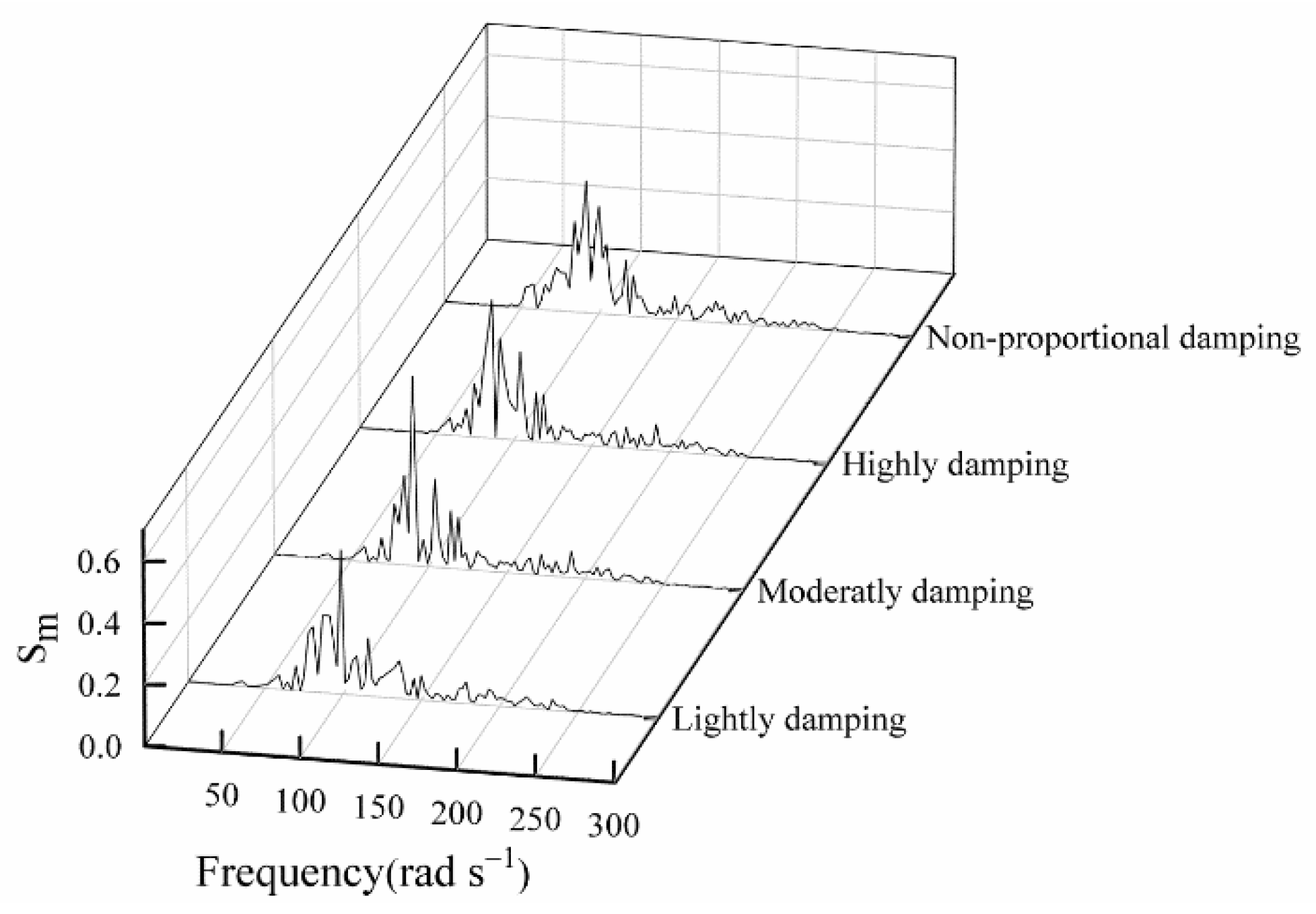
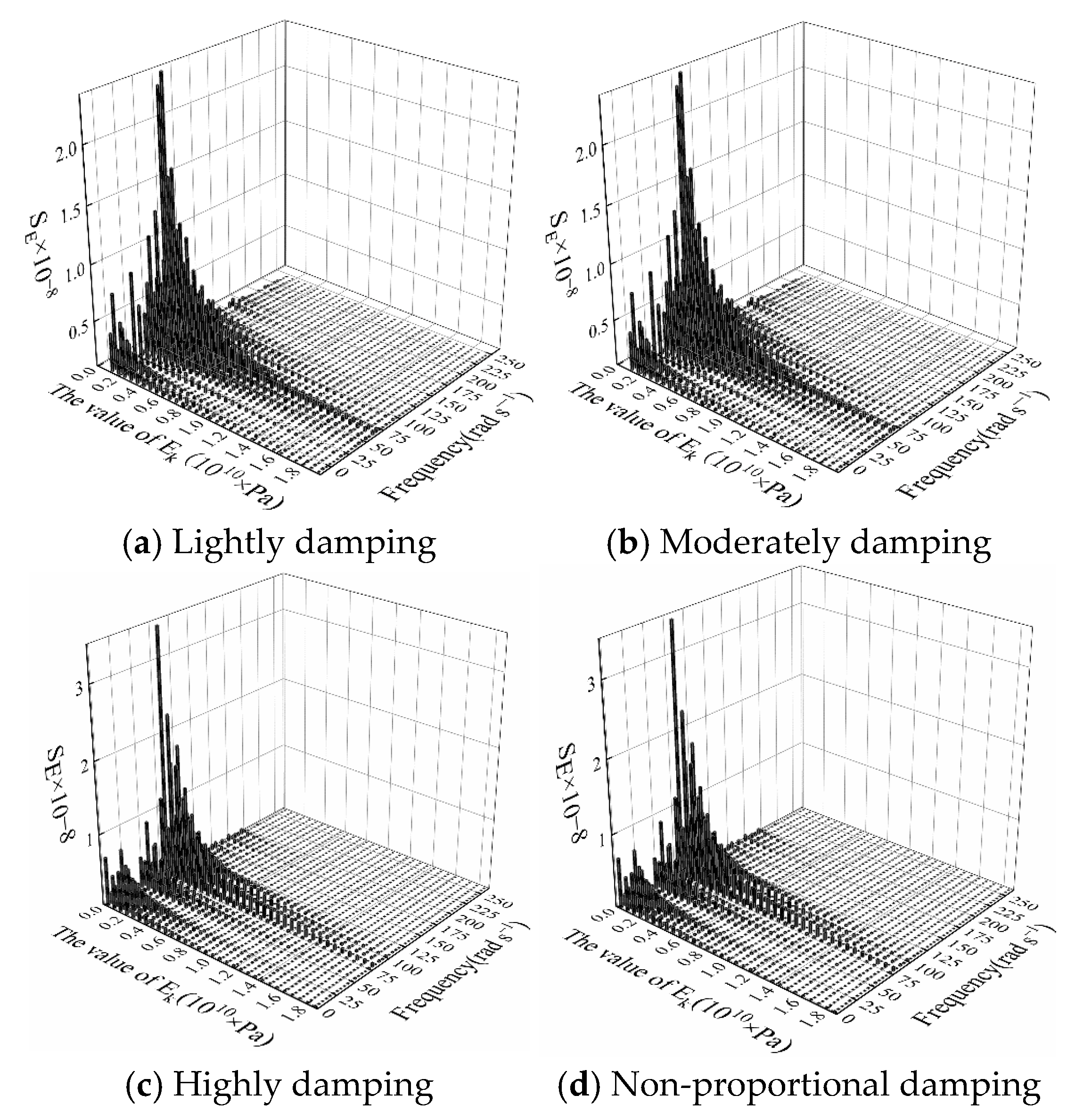
Sensitivity analysis conducted of updating parameters is needed before selecting the frequency points used for updating. The sensitivity of mf to VCEE, represented by S_m, at different damping distribution is shown in Figure 2. The sensitivity of Ek to VCEE, represented by S_E, that is a function of its own value and frequency is presented in Figure 3.

It can be observed that the magnitude of S_m is significantly larger than SE, which means that the VCEE is far more sensitive to m_f than to E_k. For m_f, the region with low sensitivity ranges between 0 and 50 rad/s. In addition, S_E approaches 0 as E_k is on the rise, i.e., now the change in E_k will not affect the VCEE. Meanwhile, m_f and E_k have highest sensitivity near the resonance frequency. Sensitivity is found to be slightly different at different damping levels. The question lies in whether frequency points in a highly sensitive region can be used in the updating process.

Firstly, the updated results corresponding to different treatment of the imaginary part are shown in

Table 5. Updated results in different imaginary parts solution methods (frequencies used for updating are in the region of 5~50 rad/s, step size is 5 rad/s).

Case No.	Solution		E2 (Pa)	E3 (Pa)	E4 (Pa)	E5 (Pa)	mf (kg)
1	Real part, discarding damping	updated results	1.488 × 1010	1.119 × 1010	1.305 × 1010	1.488 × 1010	79.55
		% deviation	0.54%	0.81%	0.77%	0.54%	0.56%
2	Modulus, discarding damping	updated results	1.522 × 1010	1.130 × 1010	1.321 × 1010	1.520 × 1010	1125.8
		% deviation	2.83%	1.80%	2.01%	2.70%	1306.25%
3	Real part, retaining damping	updated results	1.474 × 1010	1.133 × 1010	1.319 × 1010	1.477 × 1010	165.4
		% deviation	0.40%	2.07%	1.85%	0.20%	106.75%

. The frequency points applied for updating temporarily avoid the region with higher sensitivity. As shown in Table 5, only the results of case 1 are identified as acceptable, and the maximum deviation between the updated results and the simulated experimental values is shown to be 0.81%. In case 2, updated results will be subjected to severe distortion, especially in mf, suggesting that the phase spectrum will not be involved in the updating process. In case 3, only the real parts of the updated results are retained; the existence of damping matrix makes the results converge to local minimum.

In summary, the real parts of the complex acceleration response data ought to be taken as the test data and the damping matrix needs to be discarded in stage I of updating. On this basis, the principle of frequency selection is discussed by referencing the updated results under different frequency regions, as illustrated in

Table 6. Updated results in different frequency regions (frequency step size is 5 rad/s).

Case No.	Frequency Region		E2 (Pa)	E3 (Pa)	E4 (Pa)	E5 (Pa)	mf (kg)
1	5~50 rad/s	updated results	1.488 × 1010	1.119 × 1010	1.305 × 1010	1.488 × 1010	79.55
		% deviation	0.54%	0.81%	0.77%	0.54%	0.56%
2	50~120 rad/s	updated results	1.482 × 1010	1.114 × 1010	1.300 × 1010	1.482 × 1010	94.4
		% deviation	0.14%	0.36%	0.38%	0.14%	18%
3	5~120 rad/s	updated results	1.481 × 1010	1.112 × 1010	1.297 × 1010	1.481 × 1010	6.86
		% deviation	0.07%	0.18%	0.15%	0.07%	91.42%

.

For comparison purposes, the three sets of frequency regions presented in Table 6 are taken into consideration: case 1 avoids high sensitivity region; case 2 is selected from the high sensitivity region only; in case 3, all frequencies available from case 1 and case 2 are taken as reference data. It is observed that only case 1 is capable of accurately identifying the values of mf and E_k. However, it is worth noting that the value of Ek is more accurate as the frequency region is expanded. Regarding mf with a greater sensitivity than Ek, the frequency from the higher sensitivity region will give rise to a larger error. Allowing for the lack of a standard to specify whether the sensitivity is ‘high’ or ‘low’, and the satisfactory result of case 1, it is recommended to avoid the resonance frequency, that is the region with higher sensitivity. VCEE is essentially a force balance equation, and the elimination of damping affects the balance of the equation. Another advantage of the above frequency selection principle is that the effect of discarding the damping matrix on the updating process can be minimized, because the damping is the most sensitive to the resonance frequency. In addition, the results in Table 5 and Table 6 demonstrate that it is advisable to remove the degree of freedom of rotation through static condensation during the updating process.

3.2.2. The Impact of Damping Distribution

It has been proved that the damping matrix ought to be removed from Equation (1) during the identification of mass- and stiffness-related parameters. Nevertheless, it is apparent that the simulated experimental structures with different damping distribution will definitely lead to different magnitudes of seismic responses. The impact of this phenomenon on updated results will be studied in this section.

Table 7. Updated results at different damping distribution (frequencies used for updating are in the region of 5~50 rad/s, step size is 5 rad/s).

Case No.	Damping Distribution		E2 (Pa)	E3 (Pa)	E4 (Pa)	E5 (Pa)	mf (kg)
1	Lightly damping	updated results	1.486 × 1010	1.080 × 1010	1.263 × 1010	1.486 × 1010	81.55
		% deviation	0.41%	2.70%	2.47%	0.41%	1.93%
2	Moderately damping	updated results	1.488 × 1010	1.119 × 1010	1.305 × 1010	1.488 × 1010	79.55
		% deviation	0.54%	0.81%	0.77%	0.54%	0.56%
3	Highly damping	updated results	1.490 × 1010	1.121 × 1010	1.307 × 1010	1.490 × 1010	83.79
		% deviation	0.67%	0.99%	0.92%	0.67%	4.73%
4	Non-proportional damping	updated results	1.487 × 1010	1.114 × 1010	1.302 × 1010	1.488 × 1010	77.8
		% deviation	0.47%	0.36%	0.54%	0.54%	2.75%

presents the updated results at different damping distribution: case 1, 2, and 3 are proportional damping, and case 4 is non-proportional damping. It should be noted that all the deviations between the updated results and the simulated experimental values are within 5%; therefore, the results of all cases are deemed satisfactory, despite the fact that the updated results are slightly different in different cases. There is yet to be evidence suggesting that there is an intrinsic link between the difference and the damping distribution. This conclusion is drawn—damping distribution and parameters identification are independent of each other.

3.2.3. A Study with Noisy Data

In practice, the measured acceleration responses are generally affected by measurement noise. In order to check the robustness of the method under such conditions, the acceleration responses are polluted with a 5% random noise to simulate acceleration responses with noise. Due to the frequencies farther away from the resonance frequency more polluted by noise or even overwhelmed by noise, the frequencies in 60~80 rad/s are used for the updating process. The updated results for acceleration responses with noise are presented in

Table 8. Updated results for acceleration responses with noise (frequency step size is 5 rad/s).

	E2 (Pa)	E3 (Pa)	E4 (Pa)	E5 (Pa)	mf (kg)
Updated results	1.492 × 1010	1.058 × 1010	1.232 × 1010	1.434 × 1010	143.73
% deviation	0.81%	4.68%	4.86%	3.11%	79.66%

.

As shown in Table 8, the identified stiffness matrix under noise conditions remains acceptable, with a maximum deviation of 4.68% in E₃, but a 79.66% deviation in mass matrix identification due to the high sensitivity of mf. It can be seen from Table 2 that the deviation of the initial value of mf from the experimental value is as high as 828.7%. Under the same conditions, the initial value of mf is set as 100 kg and the updating process is carried out again. The updated result of mf is 75.8 kg, and the deviation from the experimental value is 5.25%. In conclusion, the proposed method has strong robustness. For parameters with high sensitivity to VCEE, the initial estimation should be as accurate as possible.

4. Shaking Table Test Study on a Load-Bearing Pipeline

Numerical simulation has shown that the damping matrix is independent of the identification of parameters related to stiffness and mass matrices. Therefore, the VCEE-based FEM updating method can be divided into two stages. The identification of mass and stiffness matrices parameters is carried out in stage I. The damping matrix is modified separately in stage II to achieve the agreement between the theoretical and measured resonance peaks. The proposed method is now evaluated for the case of a pipeline using test data.

4.1. Details of the Shaking Table Test

In order to take measurement of the seismic response, shaking table test is performed on the pipeline. Details of the experiment structure are shown in Figure 4.

It can be seen that the two pipes that make up the structure are connected by a pipe joint. The flange of the heavy 5 kg is welded to the right end of the longer pipe so that the valve can be installed in the middle of the pipeline following the pipeline system experiment.

Table 9. Performance and size of the experiment pipeline.

	Diameter	Wall Thickness	The Modulus of Elasticity	Weight
Galvanized welded pipe	48 mm	3.5 mm	2.35 × 1011 Pa	3.8 kg/m−3

shows the specifications of the test pipes.

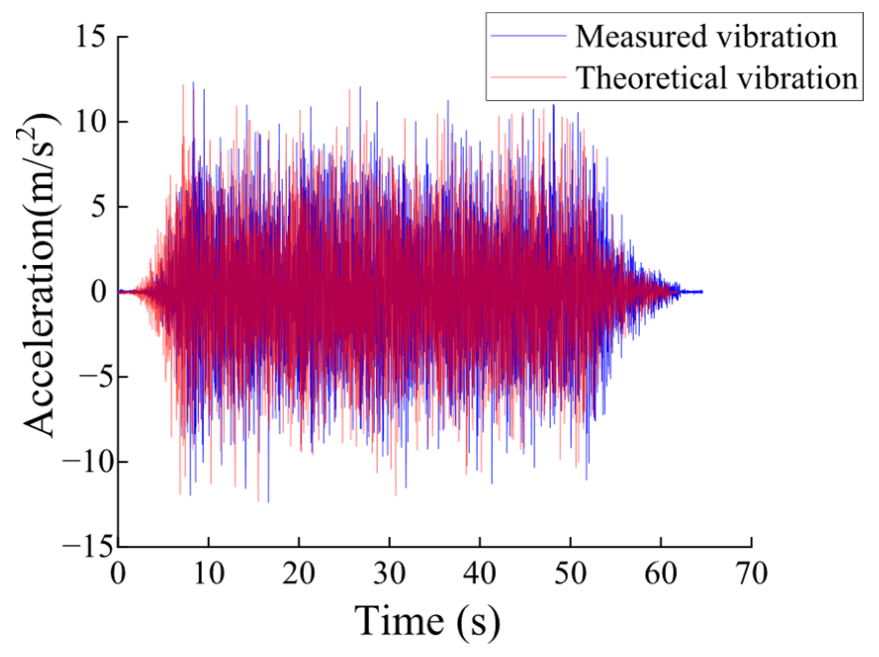
Both ends of the pipeline system are connected to the bracket by thread, and the bracket is connected to the platform of the shaking table by bolts. The brackets made of 30 mm thick steel plates welded together have sufficient stiffness to transfer the shaking table excitation to the test structure. A total of thirteen accelerometers were used to facilitate the experiment. Of them, twelve are adsorbed on the pipeline, whereas another accelerometer is adsorbed on the shaking table to monitor its acceleration time history. The acceleration seismic response measured from each point is denoted by Ai, and the subscript i represents the number of the measuring point, i = {1:13}. The accelerometers, which were used in the testing process and manufactured by Bruel and Kjaer, have a measurement range of ±100 m/s² and a factory calibration accuracy of ±2% at a 99.9% confidence level. The theoretical acceleration signals of the shaking table were compared with the measured vibration data from point A₁₃ (located at the geometric center of the shaking table surface), as shown in Figure 5.

It can be observed that the two sets of data are in close agreement, indicating that the performance of the shaking table and the accuracy of the accelerometers used in this experiment generally meet the research requirements. The horizontal artificial seismic wave was applied to the pipeline by shaking table, and the response of each measuring point was collected by the corresponding accelerometer. Detailed descriptions of the shaking table tests for this pipeline system are provided in Reference [18].

Only horizontal excitation is taken into consideration in this experiment. The pipeline structure is modeled using eleven 2D pipe elements and twelve nodes with two DOFs (translation along Y-axis and rotation around Z-axis) at each node. The lumped mass FEM corresponding to the pipeline is illustrated in Figure 6. The constraints imposed by the bracket for the pipeline were modeled as the linear elastic springs. The translation and rotation stiffness of the spring at the left and right ends are K_t1, K_r1 and K_t2, K_r2, respectively. Element 8 corresponds to the connecting portion of the two pipes in the structure.

4.2. Dynamic Stiffness Matrix Identification

4.2.1. Measurement Data Preprocessing

A₁₃ is subtracted from A₁~A₁₂ to obtain the relative acceleration response. Afterwards, the relative acceleration time history is transformed by Fourier transform to obtain the test data required for the updating process. Since the response was not measured, the rotational DOFs in the initial FEM were eliminated by Equation (16); the parameters related to the rotational DOFs were still retained.

4.2.2. Parameter Selection and Updating

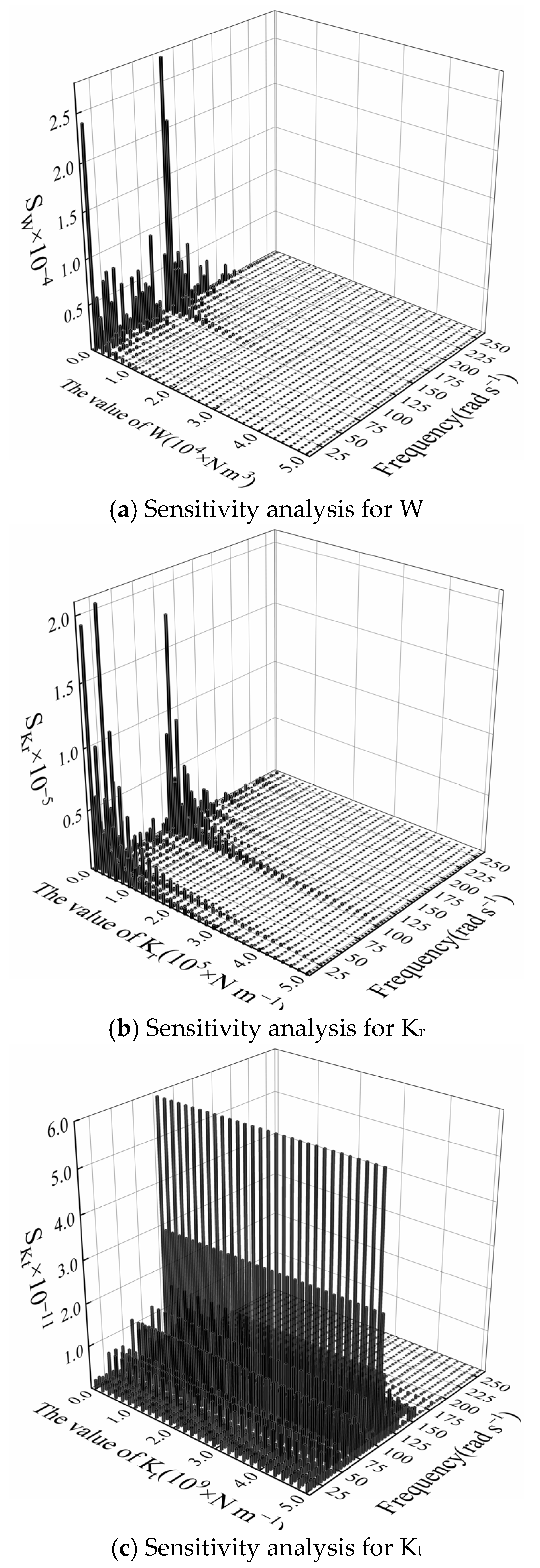
Judging the possible error source of the model combined with engineering practice experience is the first step in the selection of updating parameters. In this case, the inaccurate estimation of the stiffness of the linear spring and the bending stiffness of element 8 is the leading cause of modeling inaccuracy in FEM. The bending stiffness of element 8 is the product of its modulus of elasticity and moment of inertia, expressed in W. Due to the small weight of the pipeline, the weight assigned to each node varies only within a small range, and the weight and position of the flange are also clear, for which the mass matrix is considered to be ascertained. In order for more effective selection of the updating parameters and the frequency points to participate in updating, the sensitivity analysis of each parameter is also required to be conducted in advance of the updating. Figure 7 presents the sensitivity of W, K_t, and K_r to VCEE, respectively.

As revealed in Figure 7, the S_W and S_Kr have similar trends: there is a maximum value near 110 rad/s, which approaches 0 as the parameter value is on the rise. S_W and S_Kr also show large value within 25 rad/s, indicating that the measured data in this region were greatly affected by noise. S_Kt is noticeably less than S_W and S_Kr and is independent of the value of K_t. Thus, K_t should be removed from the updating parameters. Meanwhile, for W, which is most sensitive to VCEE, the region with low sensitivity ranges from 60 rad/s to 70 rad/s and 80 rad/s to 100 rad/s. The frequency points used for updating can be selected from this region.

Let the K_t be sufficiently large; W, K_r1, and K_r2 are identified based on Equations (13) and (14). After trial and error, the identified results for each parameter are indicated in

Table 10. Initial and final values for each parameter.

Updating Parameters	Frequency Points Used for Updating	Initial Value	Updated Value
W	60 rad/s, 65 rad/s, 68 rad/s	1 × 105 N m2	2.14 × 104 N m2
Kr1		2 × 105 N m/rad	7.787 × 105 N m/rad
Kr2		2 × 105 N m/rad	1.397 × 105 N m/rad

. It can be seen from Table 10 that the bending stiffness of element 8 is 2.14 × 10⁴ N m², while that of other pipe elements is 2.85 × 10⁴ N m², indicating a certain degree of damage at the connection part of the pipeline. The initial cognition assumed that the brackets would provide the same strength of constraint to the structure, but this was not the case. The value of K_r1 is higher than that of K_r2, which is due to the following two reasons: (1) the bracket and nut at the fixed end are hand-made and hand-tightened, as a result of which the same level of constraint cannot be guaranteed for the pipeline; (2) the length of the pipeline extending out of the bracket at the left and right ends of the system is inconsistent.

4.2.3. Damping Coefficient Identification

The energy consumption mechanism of the system is simulated by Rayleigh damping. There is always a deviation between the seismic response corresponding to the theoretical damping coefficients and the test. If the deviation is within the acceptable range, the theoretical and measured seismic response can be matched by updating the damping coefficients; otherwise, the uncertain parameters need to be identified again. In this paper, BPNN is used to update the damping coefficient. Setting element 8 has different damping coefficients.

The measured maximum responses from A₂ to A₁₁ were selected as inputs, with the damping coefficients α and β of FEM shown in Figure 5 serving as outputs. To train the BPNN model for updating the damping coefficients, the value ranges of α and β were determined by comparing the deviations between the theoretical and measured maximum responses at each measurement point. Within these ranges, 300 different combinations of damping coefficients were randomly generated, and the corresponding maximum acceleration responses at each node were calculated to form a database for training the BPNN. The network structure of the trained BPNN and the identification results of the system damping coefficients are presented in

Table 11. Parameters of the BPNN.

Input Layer	Hidden Layer	Transfer Function	Output Layer
10	28	tansig, logsig	4

and

Table 12. Updated result of damping matrix.

Element Numbers	Damping Coefficients	Value Range	Updated Result
1, 2, 3, 4, 5, 6, 7, 9, 10, 11	α	0.8~1.2	1.018
	β	6 × 10−5~9 × 10−5	8.08 × 10−5
8	α	0.8~1.2	1.018
	β	1 × 10−4~3 × 10−4	1.428 × 10−4

, respectively.

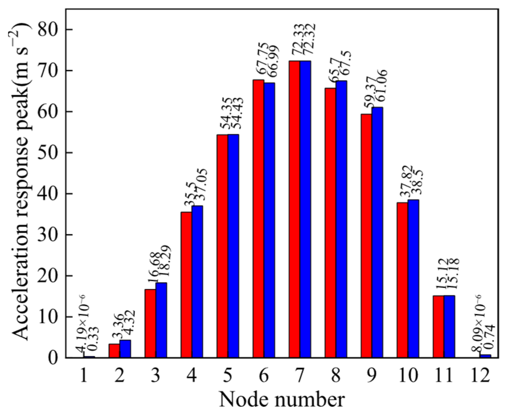
Element 8 has a larger β that conforms to the actual judgment. The comparison performed between the peak response of each node predicted by the updated model and the experimental results is shown in Figure 8.

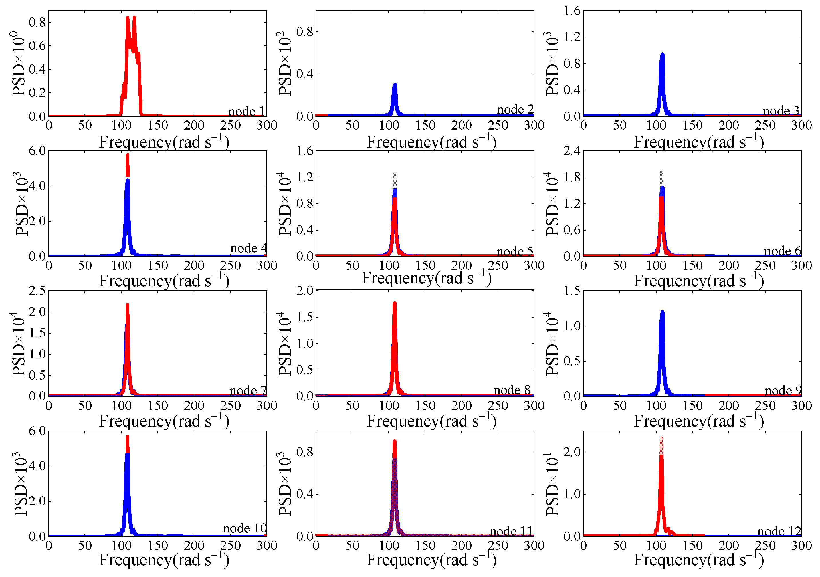
As can be seen from the figure, with the exception of A₁, A₂, and A₁₂ near the supports where significant measurement noise exists, the deviations between the theoretical and measured maximum responses at all other measurement points fall within the range of 0.33% to 5%. Moreover, the location of the system’s maximum response corresponds exactly with the experimental results. Certainly, the nature of seismic response is random vibration, as a result of which the performance of the updated model needs to be validated from other aspects. Figure 8 shows the overlay of the power spectral density (PSD) curves about the relative acceleration response of each node in the experimental and updated model.

As shown in Figure 9, the theoretical PSD curves of A₁, A₂, and A₁₂ are significantly different from the measurement results, because A₁ and A₁₂ are geometrically different from nodes 1 and 12 in FEM, and the measurement data of A₂ are greatly affected by noise. For other nodes, although the peak of the experimental PSD curve is slightly larger than the theoretical result because the initial state of the experiment structure is not ‘zero’, the PSD curves obtained by the experimental and updated models are completely consistent in shape. The phenomenon indicates that the FEM established by the VCEE-based FEM updated method perfectly replicates the test data.

5. Conclusions

In order to improve the reliability of static or dynamic analysis results by using the FE method, it is necessary to popularize the application of the FEM updating in the modeling process of mechanical structures within NPP. A VCEE-based two-stage FEM updating method is proposed in this paper. In the method, seismic response is directly used to identify uncertain parameters in the FEMs, and the measurements of FRF or modes can be avoided. A convenient way to apply FEM updating in the mechanics analysis of NPP is provided. In stage I, the optimal values of the parameters related to the mass and stiffness matrices are searched by the Marquardt method, the damping matrix is modified separately in the stage II.

Numerical simulations of the steam pipeline demonstrate the robustness and feasibility of the proposed method. The results indicate that to achieve the highest accuracy in the updated results, all imaginary components should be discarded during the parameter updating process, and the frequency points involved in the correction must avoid the resonance region. It has been confirmed by the study of shaking table test data related to pipeline that the FEM established by this method can accurately predict the dynamic characteristics of the practical structure. The deviation between the theoretical and measured peak responses at the nodes is less than 5%.

References

1. Fan, Q.Q.; Lu, Z.; Zhao, B.; Qian, J.; Jiang, D. Seismic safety evaluation and resilient analysis of nuclear containment based on failure probability. Eng. Struct. 2024, 317, 118609. [Google Scholar] [CrossRef]
2. Tang, Y.C.; Tombaş, E.; Li, C.Z. Effect of nonlinear structural response on seismic fragility and risk of emergency power supply and distribution system in a nuclear power plant. Nucl. Eng. Technol. 2025, 57, 103486. [Google Scholar] [CrossRef]
3. Shi, J.F.; Ge, Z.T.; Cao, Y.H.; Gao, J.Y.; Yu, F.; Yao, R.W. Experimental and numerical investigation on the seismic behavior of above ground high density polyethylene pipe in nuclear power plant. Structures 2024, 59, 105781. [Google Scholar] [CrossRef]
4. Sen, M. Determining Vibration Characteristics and FE Model Updating of Friction-Welded Beams. Machines 2025, 13, 653. [Google Scholar] [CrossRef]
5. Sinha, J.K.; Rao, A.R.; Sinha, R.K. Advantage of the updated model of structure: A case study. Nucl. Eng. Des. 2004, 232, 1–6. [Google Scholar] [CrossRef]
6. Sinha, J.K.; Rao, A.R.; Sinha, R.K. Realistic seismic qualification using the updated finite element model for in-core components of reactors. Nucl. Eng. Des. 2006, 236, 232–237. [Google Scholar] [CrossRef]
7. Kim, C.H.; Cha, E.J.; Shin, M. Seismic performance assessment of NPP concrete containments considering recent ground motions in South Korea. KSCE Nucl. Eng. Technol. 2022, 54, 386–400. [Google Scholar] [CrossRef]
8. ParkJ, B.; Park, N.C.; Lee, S.J.; Park, Y.P.; Choi, Y. Seismic analysis of the APR1400 nuclear reactor system using a verified beam element model. Nucl. Eng. Des. 2017, 313, 108–117. [Google Scholar] [CrossRef]
9. Chen, H.T.; Zhang, L.; Zhang, T. FRF-based model updating of liquid-filled pipeline system considering tolerance intervals of test errors in the antiresonant frequencies. Eng. Struct. 2024, 307, 117817. [Google Scholar] [CrossRef]
10. Zhao, X.Y.; Yu, K.P. Finite element model updating of damped structures using vibration test data under base excitation. J. Sound Vib. 2015, 31, 303–316. [Google Scholar] [CrossRef]
11. Lin, R.M.; Zhu, J. Finite element model updating using vibration test data under base excitation. J. Sound Vib. 2007, 303, 596–613. [Google Scholar] [CrossRef]
12. Ji, W.; Shao, T. Finite Element Model Updating for Improved Box Girder Bridges with Corrugated Steel Webs Using the Response Surface Method and Fmincon Algorithm. KSCE J. Civ. Eng. 2021, 25, 586–602. [Google Scholar] [CrossRef]
13. Abedin, M.; Basalo, F. Kian, Nafiseh. Bridge load testing and damage evaluation using model updating method. Eng. Struct. 2022, 252, 113648. [Google Scholar] [CrossRef]
14. Guan, Z.; Yang, D.; Yi, T.; Li, W.; Li, C. Bridge finite element model updating using stochastic vehicle-induced static response monitoring data. Eng. Struct. 2024, 301, 117280. [Google Scholar] [CrossRef]
15. Saidin, S.; Sakhiah, A.; Adiza, J.; Muhamad, A. Operational modal analysis and finite element model updating of ultra-high-performance concrete bridge based on ambient vibration test. Case Stud. Constr. Mater. 2022, 16, e01117. [Google Scholar] [CrossRef]
16. Fu, Y.H.; Wang, Y. Updating numerical models towards time domain alignment of structural dynamic responses with a limited number of sensors. Mech. Syst. Signal Process. 2023, 204, 110759. [Google Scholar] [CrossRef]
17. Vella, C.; Prudhomme, S. Proper generalized decomposition surrogate modeling with application to the identification of Rayleigh damping parameters. Comput. Struct. 2025, 315, 107826. [Google Scholar] [CrossRef]
18. Xue, R.Y.; Yu, S.R.; Zhang, X.H. Theoretical analysis and experimental study on the dynamic behavior of a valve pipeline system during an earthquake. Earthq. Eng. Eng. Vib. 2021, 20, 969–979. [Google Scholar] [CrossRef]
Figure 1. Details of steam pipeline (mm).
Machines 13 00987 g001
Figure 2. Sensitivity analysis for mf.
Machines 13 00987 g002
Figure 3. Sensitivity analysis for Ek.
Machines 13 00987 g003
Figure 4. Photograph of the experimental model setup on the shaking table.
Machines 13 00987 g004
Figure 5. Shaking table vibration signals, theoretical and measured.
Machines 13 00987 g005
Figure 6. The lumped mass FEM corresponding to the pipeline structure (mm).
Machines 13 00987 g006
Figure 7. Sensitivity analysis.
Machines 13 00987 g007
Figure 8. The peak of the acceleration response by analysis (represented by blue) and experiment (represented by red).
Machines 13 00987 g008
Figure 9. Overlay of PSD curves: updated FEM (represented by blue line) and experimental (represented by red line).
Machines 13 00987 g009