Chain-Based Outlier Detection: Interpretable Theories and Methods for Complex Data Scenarios ^†

Abstract

Outlier detection is a critical task in the intelligent operation and maintenance (O&M) of transportation equipment, as it helps ensure the safety and reliability of systems like high-speed trains, aircraft, and intelligent vehicles. Nearest neighbor-based detectors generally offer good interpretability, but often struggle with complex data scenarios involving diverse data distributions and various types of outliers, including local, global, and cluster-based outliers. Moreover, these methods typically rely on predefined contamination, which is a critical parameter that directly determines detection accuracy and can significantly impact system reliability in O&M environments. In this paper, we propose a novel chain-based theory for outlier detection with the aim to provide an interpretable and transparent solution for fault detection. We introduce two methods based on this theory: Cascaded Chain Outlier Detection (CCOD) and Parallel Chain Outlier Detection (PCOD). Both methods identify outliers through sudden increases in chaining distances, with CCOD being more sensitive to local data distributions, while PCOD offers higher computational efficiency. Experimental results on synthetic and real-world datasets demonstrate the superior performance of our methods compared to existing state-of-the-art techniques, with average improvements of 11.3% for CCOD and 14.5% for PCOD.

1. Introduction

Outlier detection (OD) aims to identify data points that deviate from the general data distribution. It has been proven particularly valuable in the intelligent operation and maintenance (O&M) of transportation equipment, where identifying abnormal patterns in sensor data, operational parameters, and system behaviors is essential for ensuring safety and reliability [1,2,3].

In transportation equipment monitoring, outlier detection enables early identification of mechanical anomalies such as bearing degradation, gear wear, and structural fatigue through vibration analysis and multi-sensor data fusion [4,5]. The detection of such outliers in operational parameters—including temperature fluctuations, pressure variations, and rotational speed irregularities—indicates potential mechanical failures that require immediate attention to prevent catastrophic system breakdowns [6]. Beyond traditional condition monitoring, outlier detection has been successfully applied to assess component health in rotating machinery, where abnormal vibration signatures can reveal incipient faults in bearings, shafts, and gearboxes [7,8]. In transportation-specific applications, outlier detection serves to isolate anomalous operational patterns that indicate equipment degradation or performance deviation [9,10]. This capability has proven critical in railway systems for detecting wheel-rail interaction anomalies [11,12], in aviation for identifying engine performance deviations, and in automotive systems for monitoring drivetrain irregularities [13,14].

Despite widespread applications, existing outlier detection methods face significant challenges when applied to complex data scenarios commonly encountered in transportation O&M. First, such datasets typically contain multiple outlier types simultaneously—local outliers that deviate from their neighborhoods, global outliers that are distant from the entire dataset, and cluster outliers where small clusters comprise a few outliers [15,16,17,18]. Detection strategies optimized for different outlier types may conflict with each other, leading to suboptimal performance. Second, normal operational data often exhibits non-uniform distributions, where spatially close clusters may be distant in the underlying manifold space. Existing distance-based detectors that search for neighbors in ambient space fail to capture manifold similarity, causing points in sparse operational modes to include neighbors from nearby dense clusters, thereby disrupting the underlying data structure [19]. Third, most detectors require prior specification of contamination—the expected proportion of outliers—which directly determines detection accuracy and can significantly impact system reliability in O&M environments [20,21]. Estimating contamination in dynamic transportation systems is particularly challenging due to varying operational conditions and evolving fault patterns.

This paper extends our preliminary work with substantial improvements and comprehensive evaluations [22]. We present a chain-based theory with interpretable distance analysis and manifold-aware connectivity principles for complex data scenarios. Based on this theory, we propose two chaining methods: Cascaded Chain Outlier Detection (CCOD) and Parallel Chain Outlier Detection (PCOD). CCOD employs sequential chaining where each point has one predecessor and successor, providing higher sensitivity to local distributions and better manifold structure preservation, while PCOD allows multiple successors for parallel expansion, offering superior computational efficiency and scalability for large-scale transportation monitoring applications. Both methods identify outliers through sudden increases in chaining distances without requiring contamination parameters, making them particularly suitable for dynamic O&M environments.

The remainder of this paper is organized as follows: Section 2 reviews the related work on outlier detection and the evolution of the local outlier detectors. Section 3 presents the chain-based theory of outlier detection, as well as the proposed cascaded and parallel chaining methods. Section 4 demonstrates the superiority of the proposed model using synthetic and real-life data sets. In the end, concluding remarks are given in Section 5.

2. Related Work

Over the years, various outlier detection approaches have been proposed. In this section, we give an overview of the major outlier detection methods with particular emphasis on their interpretability characteristics. We choose seven state-of-the-art algorithms as the benchmarks for our experiments in Section 4.

2.1. Nearest Neighbor-Based Methods

Among various outlier detection paradigms, nearest neighbor-based methods demonstrate the strongest interpretability due to their intuitive underlying principles: they detect outliers by evaluating local density deviations between a point and its neighbors, providing clear explanations based on neighborhood relationships that are readily understandable by domain experts [23].

The concept of Local Outlier Factor (LOF) was first proposed by Breunig [24], and it has since become a widely adopted method for local outlier detection due to its interpretable scoring mechanism. The LOF assigns outlier scores based on the ratio of a point’s k-distance to its neighbors’ average k-distance, allowing practitioners to directly understand why a point is considered anomalous by examining its local density context. However, different types of outliers may conflict with each other, where larger k-neighborhoods can detect global outliers and cluster outliers, but reduce sensitivity to local outliers. Moreover, LOF fails to capture intrinsic manifold structure, causing misclassification for linearly distributed data.

The Connectivity-based Outlier Factor (COF) [25] attempts to improve manifold sensitivity by weighting neighborhoods based on shortest connective paths rather than Euclidean distances, providing interpretable explanations through connectivity patterns that reflect data topology. However, this approach incurs high computational costs in establishing connection paths. Some methods have explored more flexible neighborhood selections while maintaining interpretability. Huang et al. [26] restrict neighborhoods to mutual k-nearest neighbors, effectively handling non-uniform densities but failing to capture manifold curvature, though the mutual neighbor concept remains intuitive for practitioners. Jin et al. [27] expand neighborhoods via Influenced Outlierness (INFLO) to k-influence spaces containing both k-nearest neighbors and reverse k-nearest neighbors, providing bidirectional neighborhood insights, but this weakens local sensitivity.

Despite their interpretability advantages, the selection of appropriate local neighborhoods in nearest neighbor methods remains challenging. Insufficient neighborhoods fail to capture complex local distributions, while excessive neighborhoods result in reduced local sensitivity.

2.2. Clustering-Based Methods

Clustering-based methods use clustering as the local neighborhood rather than the k-nearest neighbors, but typically provide less intuitive explanations compared to nearest neighbor approaches since cluster formations may not directly correspond to abnormal patterns.

The Cluster-Based Local Outlier Factor (CBLOF) [28] categorizes clusters by size and calculates outlier scores based on distance to cluster centers or nearest large clusters. While this approach offers some interpretability through cluster membership, it provides less direct explanations than neighbor-based methods. However, CBLOF’s cluster size weighting overestimates scores for points in large clusters. The Local Density Cluster-Based Outlier Factor (LDCOF) [29] addresses this by using local density instead of cluster size. Using clusters as neighborhoods can enhance similarity among neighbors, but these methods still require contamination parameters and provide less transparent decision rationales.

Density-Based Spatial Clustering of Applications with Noise (DBSCAN) identifies outliers as points that do not belong to any cluster [30,31], offering binary interpretability (cluster member vs. noise). It avoids predefined contamination, but introduces complex parameter dependencies between the neighborhood radius and minimum points, making interpretations less straightforward compared to distance-based neighbor methods.

The effectiveness of clustering-based methods is limited by their reliance on clustering information [32], which is unavailable in outlier detection tasks, and their reduced interpretability compared to direct neighbor-based approaches.

2.3. Statistics-Based Methods

Statistics-based methods assume that the given data set follows a specific distribution and identify data points that deviate from it as outliers. However, these methods often provide the least interpretable results, as their explanations rely on complex statistical concepts that may not be intuitive to domain practitioners.

Gaussian mixture models [33] detect outliers through component deviations, while Local Outlier Probabilities (LoOP) [34] assumes half-Gaussian distributions for k-nearest neighbor distances. These methods are highly sensitive to contamination and provide probabilistic explanations that may be difficult to interpret in practical maintenance scenarios. Paladimitriou et al. [35] introduce the Multi-granularity DEviation Factor (MDEF) for measuring Local Correlation Integral (LOCI). LOCI avoids contamination by statistical significance testing and addresses k-dependency by dual neighborhoods, but incurs $O\left(n^3\right)$ computational complexity while providing complex statistical explanations.

The Relative Density-based Outlier Score (RDOS) [36] uses kernel density estimation with three neighbor types to assess local density variations. The Kernel Density Estimation Based Outlier Detection (RKOF) [37] applies kernel functions for more refined local density assessment. The Copula-based Outlier Detection (COPOD) [38] utilizes empirical copulas to compute tail probabilities, leveraging negative log probabilities to effectively handle high-dimensional challenges. Similarly, the Empirical Cumulative Distribution-based Outlier Detection (ECOD) [39] ensembles empirical cumulative distributions per dimension. However, these advanced statistical methods, while mathematically sophisticated, provide explanations based on complex probability distributions that are challenging for maintenance personnel to interpret and act upon.

The effectiveness of statistics-based methods is constrained by their sensitivity to underlying manifold distributions and their limited interpretability in practical applications, which results in degraded usability when applied to complex data scenarios where clear explanations are crucial for decision-making.

3. The Proposed Methods

Empirical observations reveal that normal data points are typically concentrated in larger numbers and have sufficient neighbors within the cluster, whereas outlier data points do not conform to this pattern. To formalize this observation, we propose a chain-based theory that respects the intrinsic manifold structure of data by computing similarity via geodesic paths that approximate manifold distances. The chain distance method decomposes long distances into consecutive short paths, better adapting to the intrinsic geometric structure of the manifold. The following theorem establishes the theoretical advantage of chain distance.

Theorem 1.

Chain distance has a tighter error bound relative to k-distance. Suppose the dataset $\mathcal{X}=\left\{x_i,i=1,2,\cdots ,n\right\}$ is distributed on an m-dimensional smooth manifold $\mathcal{M}\subset {\mathbb{R}}^d$, with bounded sectional curvature, i.e., there exists a constant $\kappa >0$ such that the absolute value of sectional curvature in any direction at any point does not exceed κ. When both methods find the same k-th nearest neighbor, the error bound of the chain method is smaller than that of the k-nearest neighbor method:

$$E_c={\displaystyle \frac{d_c(x_i,x_j)-d_{\mathcal{M}}(x_i,x_j)}{d_{\mathcal{M}}(x_i,x_j)}}\le E_k={\displaystyle \frac{d_k(x_i,x_j)-d_{\mathcal{M}}(x_i,x_j)}{d_{\mathcal{M}}(x_i,x_j)}}$$

(1)

where $x_i,x_j\in \mathcal{X}$, and $x_i$ is the k-th nearest neighbor of $x_j$. $d_k(x_i,x_j)=\parallel x_i-x_j\parallel$ represents the distance estimation of k-nearest neighbor, i.e., the Euclidean distance from $x_i$ to its k-th nearest neighbor $x_j$; $d_c(x_i,x_j)={\sum }_{t=1}^{k-1}\parallel x^t-x^{t+1}\parallel$ represents the chain distance from $x_i$ to $x_j$, i.e., the cumulative distance of piecewise paths for the set $\{x^1=x_i,x^2,\dots ,x^k=x_j\}$ constructed by stepwise nearest neighbor linking; $d_{\mathcal{M}}(x_i,x_j)$ represents the geodesic distance between $x_i$ and $x_j$.

Proof. 

We will analyze the local error bounds for k-nearest neighbor distance and chain distance separately, and then compare them.

• Step 1. Local error bound for k-distance: For data point pairs p and q within the neighborhood, by the arc-chord estimation inequality in Riemannian geometry:

  $$\parallel p-q\parallel \le d_{\mathcal{M}}(p,q)\le \parallel p-q\parallel \left(1+{\displaystyle \frac{{\kappa \parallel p-q\parallel }^2}{6}}\right)$$

  (2)

  Taking $p=x_i$, $q=x_j$, and denoting $s=\parallel x_i-x_j\parallel$, we have:

  $$0\le d_{\mathcal{M}}(x_i,x_j)-d_k(x_i,x_j)\le {\displaystyle \frac{\kappa }{6}}{s}^3$$

  (3)

  Therefore, the relative error $E_k$ of the k-distance satisfies:

  $${\displaystyle \frac{d_k(x_i,x_j)-d_{\mathcal{M}}(x_i,x_j)}{d_{\mathcal{M}}(x_i,x_j)}}\le {\displaystyle \frac{\kappa s^2}{6}}\left(1+O\left(\kappa s^2\right)\right)$$

  (4)
• Step 2. Local error bound for chain distance: The chain distance $d_c(x_i,x_j)$ decomposes long distances into multiple short segments, reaching the same $x_j$ through stepwise nearest neighbor linking. The distance between adjacent point pairs $x^t$ and $x^{t+1}$ in the chain is sufficiently small. Taking $p=x^t$, $q=x^{t+1}$, the error for local link sets in the chain path is:

  $$d_{\mathcal{M}}(x^t,x^{t+1})-\parallel x^t-x^{t+1}\parallel \le {\displaystyle \frac{\kappa {\epsilon }_t^3}{6}}$$

  (5)

  where ${\epsilon }_t=\parallel x^t-x^{t+1}\parallel$. The total error of chain distance is:

  $$d_c(x_i,x_j)-d_{\mathcal{M}}(x_i,x_j)\le \sum _{t=1}^{k-1}{\displaystyle \frac{\kappa {\epsilon }_t^3}{6}}\le {\displaystyle \frac{\kappa {\overline{\epsilon }}_t^2}{6}}$$

  (6)

  where ${\overline{\epsilon }}_t={\displaystyle \frac{1}{k-1}}{\sum }_{t=1}^{k-1}{\epsilon }_t$. Therefore, the relative error $E_c$ of chain distance is:

  $${\displaystyle \frac{d_c(x_i,x_j)-d_{\mathcal{M}}(x_i,x_j)}{d_{\mathcal{M}}(x_i,x_j)}}\le {\displaystyle \frac{\kappa {\overline{\epsilon }}_t^2}{6}}$$

  (7)
• Step 3. Comparison of the two methods: When there exists at least one segment ${\epsilon }_t\le s$, the relative error upper bound of the chain method is strictly smaller than that of the k-nearest neighbor method:

  $$E_c={\displaystyle \frac{\kappa {\overline{\epsilon }}_t^2}{6}}\le E_k={\displaystyle \frac{\kappa s^2}{6}}$$

  (8)

□

The chain-based theory enables us to distinguish normal points from outliers based on their chaining behavior. It is assumed that for a normal data point, there should exist a sufficient number of points in its neighborhood such that a series of chaining distances starting from this point does not increase excessively. Conversely, for an outlier data point, the number of points in its neighborhood is insufficient to prevent excessive increases in chaining distances.

As shown in Figure 1, the chain-based theory aims to chain normal points (green dots) following the manifold structure, while leaving outliers unchained as they cause excessive increases in chaining distances. However, traditional density-based methods search for neighbors in ambient space, and outliers can be selected as neighbors due to their proximity in ambient distance.

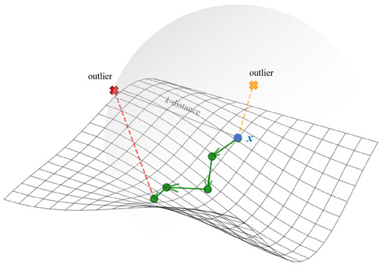
Figure 1. An illustration of chain-based theory.

Therefore, we utilize the chaining distance as an estimator of data distribution, searching neighbors via consecutive short paths that approximate manifold distances. Points whose chaining distances exhibit excessive increases are identified as outliers, indicating significant separation from neighbors in manifold geometry. Conversely, chained data points with stable chaining distance are identified as the potential normal data. Based on this chain-based theory, two methods are proposed for outlier detection.

3.1. Cascaded Chain Outlier Detection

Suppose $\mathcal{X}=\left\{x_i,i=1,2,\cdots ,n\right\}$ is the given data set, ${\mathcal{X}}_N=\left\{\right\}$ is the data set of normal points, and ${\mathcal{X}}_O=\left\{\right\}$ is the data set of outlier points. Use the Euclidean distance as the distance measure between any two points, i.e., $d\left(x_i,x_{\overline{i}}\right)=\sqrt{{x_i}^2+{x_{\overline{i}}}^2}$, where $x_i,x_{\overline{i}}\in \mathcal{X}$, and $i\ne \overline{i}$, and calculate this distance only once. At the beginning of a chaining process in the search for outliers, select a random data point $x_i$ from ${\mathcal{X}}_S$ as the start point and initialize the current chain as, i.e., ${\mathcal{X}}_C=\left\{x_i^j\right\}$ with $x_i^1=x_i$. It is the first point in the current chain, and any point can serve as a start point, provided it has not already been identified as normal or used as a start point. Thus, we define a data set of the remaining start points as ${\mathcal{X}}_S=\mathcal{X}-{\mathcal{X}}_N-\left\{x_i^j\right\}$. Then, the second data point $x_i^2$ to be included in the current chain is chosen from $\left(\mathcal{X}-\left\{x_i^j\right\}\right)$, which has the smallest distance to the start point $x_i^1$. If there are multiple points with the minimum distance from the start point, only one is selected. The smallest distance between $x_i^1$ and $x_i^2$ is defined as a chaining distance $d_1^2$, i.e., $d_1^2=d\left(x_i^1,x_i^2\right)$. It is the second point in the current chain, i.e., ${\mathcal{X}}_C={\mathcal{X}}_C\cup \left\{x_i^2\right\}$. For $j\ge 2$, select the $j+1$-th data point from $\left(\mathcal{X}-\left\{x_i^j\right\}\right)$ which has the smallest Euclidean distance to the j-th data point $x_i^j$. The ratio of the chaining distance $d_j^{j+1}$ over the average chaining distance in the current chain is calculated as

$$r_i^{j+1}={\displaystyle \frac{d_j^{j+1}}{\left({\displaystyle \sum _{j=1}^j}{d}_{j-1}^j\right)/\left(j-1\right)}}.$$

(9)

For $j<k$, if the $x_i^{j+1}$ satisfies

$${\displaystyle \frac{1}{\gamma }}\le r_i^{j+1}\le \gamma ,$$

(10)

means that including $x_i^{j+1}$ in the series of chaining distances does not cause excessive increases, and $x_i^{j+1}$ is a potential normal data point that can be added to the current chain, i.e., ${\mathcal{X}}_C={\mathcal{X}}_C\cup \left\{x_i^{j+1}\right\}$, and let $j=j+1$ to chain the next point.

If ${\displaystyle \frac{1}{\gamma }}>r_i^{j+1}$ and $r_i^{j+1}\le \gamma$ in the case of $j<k$, consider the possible merging of two chains. Set the pre-chain data set ${\tilde{\mathcal{X}}}_C={\mathcal{X}}_C$, $x_i^{\tilde{j}+1}=x_i^{j+1}$, and start a new chain from $x_i^{j+1}$, ${\mathcal{X}}_C=\left\{\right\}$, $j=1$, $x_i^1=x_i^{\tilde{j}+1}$. Once $|{\mathcal{X}}_C|+|{\tilde{\mathcal{X}}}_C|\ge k$ and satisfies the condition as follows:

$${\displaystyle \frac{1}{\gamma }}\le {\displaystyle \frac{\left({\displaystyle \sum _{\tilde{j}=1}^{\tilde{j}}}{d}_{\tilde{j}-1}^{\tilde{j}}\right)/\left(\tilde{j}-1\right)}{\left({\displaystyle \sum _{j=1}^j}{d}_{j-1}^j\right)/\left(j-1\right)}}\le \gamma ,$$

(11)

these two chains have similar densities that can be combined as ${\mathcal{X}}_C={\mathcal{X}}_C\cup {\tilde{\mathcal{X}}}_C$, $j=|{\tilde{\mathcal{X}}}_C|+j$, and let $j=j+1$ to chain the next point; If $|{\mathcal{X}}_C|+|{\tilde{\mathcal{X}}}_C|\ge k$ and Equation (11) is not satisfied, it means that the two chains have different densities and cannot be combined, thus the pre-chain is reset as ${\tilde{\mathcal{X}}}_C=\left\{\right\}$ and let $j=j+1$ to chain the next point.

If $r_i^{j+1}>\gamma$, it means that the chaining distances of $x_i^{j+1}$ increase excessively, and the current chain process ends at $x_i^j$. In the case of $j<k$, ${\mathcal{X}}_C$ is not considered a normal cluster and is discarded. A new chaining process begins with ${\mathcal{X}}_C=\left\{\right\}$ from a random point in ${\mathcal{X}}_S$.

Note that the proposed method imposes stricter constraints in the case of $j<k$, in which the upper constraint $\gamma$ aims to prevent the chain from cascading to outliers or other clusters, while the lower constraint ${\displaystyle \frac{1}{\gamma }}$ is to prevent the start point from being an outlier. If the start point is an outlier, the chaining distance of $x_i^j\left(j>2\right)$ would increase excessively compared to that of $x_i^2$. However, if $j\ge k$, the start point must not be an outlier, because the proposed method considers chains containing more than K elements to be normal, making the lower bound constraint unnecessary.

For $j\ge k$, if $x_i^{j+1}$ satisfies $r_i^{j+1}\le \gamma$, it means that including $x_i^{j+1}$ in the series of chaining distances does not cause excessive increases, and $x_i^{j+1}$ is a potential normal data point that can be added to the current chain, i.e., ${\mathcal{X}}_C={\mathcal{X}}_C\cup \left\{x_i^{j+1}\right\}$, and let $j=j+1$ to chain the next point; If $r_i^{j+1}>\gamma$, it means that the chaining distances of $x_i^{j+1}$ increase excessively, and the current chain process ends at $x_i^j$. ${\mathcal{X}}_N={\mathcal{X}}_N\cup {\mathcal{X}}_C$, and the data set of start points is updated as ${\mathcal{X}}_S={\mathcal{X}}_S-{\mathcal{X}}_N$. A new chaining process begins with ${\mathcal{X}}_C=\left\{\right\}$ from a random point in ${\mathcal{X}}_S$.

The search stops when no new clusters can be formed, i.e., $|{\mathcal{X}}_S| =0$. Finally, a point is considered normal if it belongs to ${\mathcal{X}}_N$ and considered an outlier if it does not belong to ${\mathcal{X}}_N$, i.e., ${\mathcal{X}}_O=\mathcal{X}-{\mathcal{X}}_N$. In the proposed method, every chained point has only one predecessor and one successor, excluding the first and last. Hence, we refer to the method as outlier detection by cascaded chaining. The process of detecting the outliers by CCOD is summarized in Algorithm 1.

Algorithm 1: Outlier detection by cascaded chaining

Input:  The given data set $\mathcal{X}=\left\{x_i,i=1,2,\cdots ,n\right\}$, and a integer parameter $k\left(2<k\ll n\right)$, a real parameter $\gamma (\gamma \ge 1)$, and a real parameter $\alpha \left(0<\alpha <1\right)$;   1:  Initialize: chain data set ${\mathcal{X}}_C=\left\{\right\}$, pre-chain data set ${\tilde{\mathcal{X}}}_C=\left\{\right\}$, start point data set ${\mathcal{X}}_S=\mathcal{X}$, normal data set ${\mathcal{X}}_N=\left\{\right\}$, and outlier data set ${\mathcal{X}}_O=\left\{\right\}$;   2:  while  $|{\mathcal{X}}_S| >0$  do   3:     Take $x_i$ from ${\mathcal{X}}_S$ randomly as a start point, $j=1$, $x_i^j=x_i$, ${\mathcal{X}}_C=\left\{x_i^j\right\}$, ${\mathcal{X}}_S={\mathcal{X}}_S-{\mathcal{X}}_N-\left\{x_i^j\right\}$   4:     $x_i^{j+1}=arg{min}_{x_i\in (\mathcal{X}-\left\{x_i^j\right\})}d(x_i^j,x_i)$   5:      if $j<2$ then   6:         ${\mathcal{X}}_C={\mathcal{X}}_C\cup \left\{x_i^{j+1}\right\}$, $j=j+1$, go to 4   7:     else   8:        if $|{\mathcal{X}}_C|\ge k$ and $r_i^{j+1}\le \gamma$ then   9:            ${\mathcal{X}}_C={\mathcal{X}}_C\cup \left\{x_i^{j+1}\right\}$, $j=j+1$,  10:            ${\mathcal{X}}_N={\mathcal{X}}_N\cup {\mathcal{X}}_C$, go to 4  11:       else if $|{\mathcal{X}}_C| <k$ and ${\displaystyle \frac{1}{\gamma }}\le r_i^{j+1}\le \gamma$ then  12:          ${\mathcal{X}}_C={\mathcal{X}}_C\cup \left\{x_i^{j+1}\right\}$, $j=j+1$, go to 4  13:       else if $|{\mathcal{X}}_C| <k$ and $r_i^{j+1}\le \gamma$ then  14:          ${\tilde{\mathcal{X}}}_C={\mathcal{X}}_C$, $x_i^{\tilde{j}+1}=x_i^{j+1}$,  15:          ${\mathcal{X}}_C=\left\{\right\}$, $j=1$, $x_i^1=x_i^{\tilde{j}+1}$, go to 4  16:       else if ${\tilde{\mathcal{X}}}_C\ne \left\{\right\}$ and $|{\mathcal{X}}_C|+|{\tilde{\mathcal{X}}}_C |\ge \lceil \alpha \times k^2\rceil$ then  17:          if satisfy Equation (11) then  18:            ${\mathcal{X}}_C={\mathcal{X}}_C\cup {\tilde{\mathcal{X}}}_C$, $j=|{\tilde{\mathcal{X}}}_C|+j$, $j=j+1$,  19:            ${\mathcal{X}}_N={\mathcal{X}}_N\cup {\mathcal{X}}_C$, go to 4  20:          else  21:            ${\tilde{\mathcal{X}}}_C=\left\{\right\}$, $j=j+1$, go to 4  22:          end if  23:       else  24:          ${\mathcal{X}}_C=\left\{\right\}$  25:       end if  26:     end if  27:   end while Output:  ${\mathcal{X}}_O=\mathcal{X}-{\mathcal{X}}_N$

To illustrate the process of how CCOD forms chains, we present an example of a two-dimensional data set in Figure 2. The parameters ARE $k=5$ and $\gamma =1.5$. Starting at the point $x_1$, the second point in the chain is identified as $x_3$, as it has the smallest distance from $x_1$, i.e., $x_3^2=x_3$. Next, the point $x_7$ is cascaded as the successor of $x_3^2$, i.e., $x_7^3=x_7$, because there are sufficient points in its neighborhood and the chaining distance condition ${\displaystyle \frac{1}{\gamma }}\le r_7^3\le \gamma$ is satisfied. Similarly, $x_9^4$ is cascaded as the successor of $x_7^3$. The current chain ${\mathcal{X}}_C$ is $\{x_1^1,x_3^2,x_7^3,x_9^4\}$. Then, we focus on the nearest point to $x_9^4$, which is $x_{15}$ and has a much shorter chain distance than before, i.e., ${\displaystyle \frac{1}{\gamma }}>r_{15}^5$ and $r_{15}^5\le \gamma$. At this point, we consider merging two chains. We copy the current chain into a pre-chain denoted as ${\tilde{\mathcal{X}}}_C=\{x_1^1,x_3^2,x_7^3,x_9^4\}$ and a new current chain starts from $x_{15}$. The search stops once $|{\mathcal{X}}_C|+|{\tilde{\mathcal{X}}}_C|\ge k$, and the ${\mathcal{X}}_C=\{x_{15}^1,x_{18}^2,x_{19}^3\}$. The current chain and pre-chain can be combined because they have similar densities according to Equation (11), i.e., ${\mathcal{X}}_C={\mathcal{X}}_C\cup {\tilde{\mathcal{X}}}_C$, and the order of the data points in ${\mathcal{X}}_C$ is updated as $\{x_1^1,x_3^2,x_7^3,x_9^4,x_{15}^5,x_{18}^6,x_{19}^7\}$. For $|{\mathcal{X}}_C|>k$, the $x_{20}^8$ is cascaded as the successor of $x_{19}^7$, but $x_{21}$ as the nearest point of $x_{20}^8$ cannot be cascaded, because it would increase the chaining distance excessively, i.e., $r_{21}^9>\gamma$. At this point, the current chain is formed, as it cannot be extended any further. The current chain is considered a normal data set, as it contains more than k data points. However, $x_{21}$ fails to be chained as a successor and cannot form a normal data set as a start point, and thus would be considered an outlier.

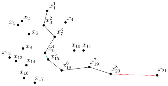
Figure 2. CCOD in a 2D example.

It should be noted that in Figure 2, a substantial number of normal data points persist unchained even after undergoing a chaining process. These data points possess adequate neighbors but are restricted by the expansion direction of the current chain. Hence, we propose a variant approach that allows each point to have multiple successors. The CCOD approach is a special case of the deformation method, where the number of successor points is restricted to 1. While the two methods differ in detail, they share the same underlying concept of identifying outliers with excessive increases in chain distances and collecting the chained data points into a cluster of potential normal data when the chaining process exhibits no excessive distance change. Next, the potential normal data cluster would be defined as a normal data set if it contains more than $\lceil \alpha \times k^2\rceil \left(0<\alpha <1\right)$ data points.

3.2. Parallel Chain Outlier Detection

Suppose $\mathcal{X}=\left\{x_i,i=1,2,\cdots ,n\right\}$ is the given data set, ${\mathcal{X}}_N=\left\{\right\}$ is the data set of normal points, and ${\mathcal{X}}_O=\left\{\right\}$ is the data set of outlier points. We still use the Euclidean distance as the distance measure between any two points. At the beginning of a chaining process, select a random data point $x_i$ from ${\mathcal{X}}_S$ as the start point and initialize the current chain as ${\mathcal{X}}_C=\left\{x_i^j\right\}$ with $x_i^1=x_i$. It is the first point in the current chain, and any point can serve as a start point, provided it has not already been identified as normal or used as a start point. Thus, we define a data set of the remaining start points as ${\mathcal{X}}_S=\mathcal{X}-{\mathcal{X}}_N-\left\{x_i^j\right\}$. Then, the next batch of points is chosen from $\left(\mathcal{X}-\left\{x_i^j\right\}\right)$ such that they have the first K smallest distances to the start point $x_i^1$. If there are more than k following points for one data point, only the first k points are included. The distance between $x_i^1$ and $x_i^j$ is defined as a chaining distance $d_1^j$, i.e., $d_1^j=d\left(x_i^1,x_i^j\right)$. Let ${\mathcal{X}}_B^z$ represent the z-th batch. The first batch contains only a start point, i.e., ${\mathcal{X}}_B^1=\left\{x_i^1\right\}$, and the second batch is recorded as ${\mathcal{X}}_B^2$, i.e., ${\mathcal{X}}_B^2=\{x_i^2,\cdots ,x_i^{k+1}\}$ where $x_i^j\in \mathcal{X}-\left\{x_i^1\right\}$ and $d(x_i^1,x_i^j)\le d(x_i^1,x_i^{j+1})$. These two batches are included in the current chain, i.e., ${\mathcal{X}}_C={\mathcal{X}}_B^1\cup {\mathcal{X}}_B^2$. For $z\ge 3$, the current points are selected from ${\mathcal{X}}_B^z$ in ascending order of superscript, and the k nearest points to be included in the $z+1$-th batch are selected from $\mathcal{X}-{\mathcal{X}}_C$ based on their k smallest Euclidean distances to the current point. The t-th nearest point to the current point $x_i^j$ is $x_i^{j+t}$, where $t=1,\dots ,k$. The ratio of the chaining distance $d_j^{j+t}$ over the average chaining distance in the current chain is calculated as

$$r_i^{j+t}={\displaystyle \frac{d_j^{j+t}}{\left({\displaystyle \sum _{j=1}^j}{d}_j^{j-1}\right)/\left(j-1\right)}},$$

(12)

Note that points with smaller distances to their predecessors have higher priority in selecting successors, since each successor can only be selected once within the same batch or cluster.

For $t=1,\dots ,k$, if any $x_i^{j+t}$ satisfies

$${\displaystyle \frac{1}{\gamma }}\le r_i^{j+t}\le \gamma ,$$

(13)

it means that a series of chaining distances containing the $x_i^{j+t}$ does not increase excessively, and the $x_i^{j+t}$ is a potential normal data point that can be taken into the $z+1$-th batch as one of the successor points of $x_i^j$, i.e., $x_i^{j+1}=x_i^{j+t}$, ${\mathcal{X}}_B^{z+1}={\mathcal{X}}_B^{z+1}\cup \left\{x_i^{j+1}\right\}$ and let $j=j+1$ to chain the next point. Then, ${\mathcal{X}}_C={\mathcal{X}}_C\cup {\mathcal{X}}_B^{z+1}$, and let $z=z+1$ to chain the next batch. The current chain process stops when there are no new points to be chained, i.e., ${\mathcal{X}}_C\cup {\mathcal{X}}_B^{z+1}=\left\{\right\}$. Then, the ${\mathcal{X}}_C$ is a normal cluster if $j\ge \lceil \alpha \times k^2\rceil \left(0<\alpha <1\right)$, such that ${\mathcal{X}}_N={\mathcal{X}}_N\cup {\mathcal{X}}_C$, and the data set of start points is updated as ${\mathcal{X}}_S={\mathcal{X}}_S-{\mathcal{X}}_N$. A new chaining process begins with ${\mathcal{X}}_C=\left\{\right\}$ from a random point in ${\mathcal{X}}_S$.

The search stops when no new clusters can be formed, i.e., $|{\mathcal{X}}_S| =0$. Finally, a point is considered normal if it belongs to ${\mathcal{X}}_N$; Otherwise, it is considered an outlier, i.e., ${\mathcal{X}}_O=\mathcal{X}-{\mathcal{X}}_N$. In the proposed variant approach, except for the start point, each chain point has only one predecessor, but can have more than one successor. Hence, we refer to the method as outlier detection by parallel chaining. The process of detecting the outliers by PCOD is summarized in Algorithm 2.

To illustrate the process of how PCOD forms chains, we present an example of a two-dimensional data set in Figure 3. The parameters $k=5$ and $\gamma =1.5$. Starting at the point $x_1$ as the first batch ${\mathcal{X}}_B^1=x_1^1$, the second batch points in the chain are identified as $x_3,x_4,x_2,x_6$ and $x_5$, as they have the k smallest distance from $x_1$ and $d_1^3<d_1^4<d_1^2<d_1^6<d_1^5$, i.e., ${\mathcal{X}}_B^2=\{x_3^2,x_4^3,x_2^4,x_6^5,x_5^6\}$. The current chain is ${\mathcal{X}}_C={\mathcal{X}}_B^1\cup {\mathcal{X}}_B^2$. Next, $x_7$ is chained as the successor of $x_3^2$ from $\mathcal{X}-{\mathcal{X}}_C$, i.e., $x_7^7=x_7$, and $x_8$ is chained as the successor of $x_6^5$ from $\mathcal{X}-{\mathcal{X}}_C$, i.e., $x_8^8=x_8$, as ${\displaystyle \frac{1}{\gamma }}\le r_7^7\le \gamma$ and ${\displaystyle \frac{1}{\gamma }}\le r_8^8\le \gamma$. However, the other points in ${\mathcal{X}}_B^2$ have no new successors, so the 3-rd batch has two elements, i.e., ${\mathcal{X}}_B^3=\{x_7^7,x_8^8\}$. The current chain is ${\mathcal{X}}_C={\mathcal{X}}_C\cup {\mathcal{X}}_B^3$. Similarly, $x_9^9,x_{10}^{10}$, and $x_{11}^{11}$ are chained as successors of $x_7^7$ from $\mathcal{X}-{\mathcal{X}}_C$, and $x_{12}^{12},x_{13}^{13}$ and $x_{14}^{14}$ are chained as successors of $x_8^8$ from $\mathcal{X}-{\mathcal{X}}_C$. The 4-th batch ${\mathcal{X}}_B^4$ is $\{x_9^9,x_{10}^{10},x_{11}^{11},x_{12}^{12},x_{13}^{13},x_{14}^{14}\}$, and the current chain is ${\mathcal{X}}_C={\mathcal{X}}_C\cup {\mathcal{X}}_B^4$. Continuing in the same way, $x_{15}^{15}$ is chained as the successors of $x_9^9$, $x_{18}^{16}$ are chained as successors of $x_{10}^{10}$, $x_{19}^{17}$ are chained as successors of $x_{11}^{11}$, and $x_{16}^{18},x_{17}^{19}$ are chained as successors of $x_{14}^{14}$. The 5-th batch ${\mathcal{X}}_B^5$ is $\{x_{15}^{15},x_{18}^{16},x_{19}^{17},x_{16}^{18},x_{17}^{19}\}$, and the current chain is ${\mathcal{X}}_C={\mathcal{X}}_C\cup {\mathcal{X}}_B^5$. The 6-th batch ${\mathcal{X}}_B^6$ is $\left\{x_{20}^{20}\right\}$, which only has one element as the successors of $x_{19}^{17}$. However, $x_{21}$ fails to be chained as a successor and cannot form a normal data set as a start point, and thus would be considered an outlier.

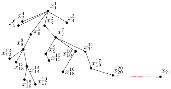
Figure 3. PCOD in a 2-D example [22].

Both CCOD and PCOD have a theoretical time complexity of $\mathrm{O}\left(n^2\right)$, but their practical performance differs due to chain formation strategies. CCOD requires a large number of small chains, providing higher sensitivity to local distributions but making it unsuitable for large data sets. PCOD divides observations into fewer chains with more points in each chain, offering superior computational efficiency by greatly reducing the time required to form new chains, though more time is spent processing each individual chain. Therefore, CCOD is more suitable for small data sets requiring precise local analysis, while PCOD is ideal for large data sets prioritizing computational efficiency.

Algorithm 2: Outlier detection by parallel chaining

Input:   The given data set $\mathcal{X}=\left\{x_i,i=1,2,\cdots ,n\right\}$, and a integer parameter $k\left(2<k\ll n\right)$, a real parameter $\gamma (\gamma \ge 1)$, and a real parameter $\alpha \left(0<\alpha <1\right)$.   1:  Initialize: chain data set ${\mathcal{X}}_C=\left\{\right\}$, start point data set ${\mathcal{X}}_S=\mathcal{X}$, normal data set ${\mathcal{X}}_N=\left\{\right\}$, outlier data set ${\mathcal{X}}_O=\left\{\right\}$;   2:  while  $|{\mathcal{X}}_S|>0$  do   3:     Take $x_i$ from ${\mathcal{X}}_S$ randomly as a start point, $j=1$, $x_i^j=x_i$, $z=1$, ${\mathcal{X}}_B^z=\left\{x_i^j\right\}$, ${\mathcal{X}}_C={\mathcal{X}}_B^z$, ${\mathcal{X}}_S={\mathcal{X}}_S-{\mathcal{X}}_N-{\mathcal{X}}_B^z$   4:     while $|{\mathcal{X}}_B^z|>0$ do   5:        for $\widehat{t}=1:\left|{\mathcal{X}}_B^z\right|$ do   6:           for $t=1:k$ do   7:             $x_i^{j+t}=arg{min}_{x_i^{j+t}\in (\mathcal{X}-{\mathcal{X}}_C),x_i^{\widehat{t}}\in {\mathcal{X}}_B^z}d(x_i^{\widehat{t}},x_i^{j+t})$   8:             if $|{\mathcal{X}}_C|==1$ or $x_i^{j+t}$ satisfies Equation (13) then   9:                ${\mathcal{X}}_B^{z+1}={\mathcal{X}}_B^{z+1}\cup \left\{x_i^{j+1}\right\}$, $j=j+1$  10:             end if  11:           end for  12:        end for  13:        ${\mathcal{X}}_C={\mathcal{X}}_C\cup {\mathcal{X}}_B^{z+1}$, $z=z+1$, ${\mathcal{X}}_B^{z+1}=\left\{\right\}$  14:      end while  15:      if $|{\mathcal{X}}_C|\ge \lceil \alpha \times k^2\rceil$ then  16:        ${\mathcal{X}}_N={\mathcal{X}}_N\cup {\mathcal{X}}_C$  17:      else  18:        ${\mathcal{X}}_C=\left\{\right\}$  19:      end if  20:  end while Output:  ${\mathcal{X}}_O=\mathcal{X}-{\mathcal{X}}_N$

4. Results

In this section, we compare the proposed models with seven state-of-the-art algorithms. To ensure a comprehensive comparison, we chose LOF [24] and its most-cited variants COF [25], LoOP [34], LOCI [35], NOF [26], RDOS [36], and ECOD [39] as representative local outlier detectors. Unlike existing methods requiring predefined contamination parameters, our approaches automatically identify outliers by detecting abrupt increases in chaining distances.

The performance metric employed in our study is the Area Under the Receiver Operating Characteristic Curve (AUC) and Precision (PRN). The AUC evaluates the trade-off between correctly identifying true outliers and minimizing false detections on normal points, where AUC = 1.00 indicates perfect detection performance to identify normal data and outliers. Unlike conventional detectors that produce continuous outlier scores and require a predefined contamination, the proposed methods output binary scores, assigning 1 to predicted normal points and 0 to predicted outliers. The PRN measures the proportion of correctly identified outliers among all predicted outliers, where PRN = 1.00 indicates that all predicted outliers are true outliers. All methods in our study achieved the highest AUC based on their respective parameters. All reported results are averaged over 5 independent runs.

Experiments are conducted on a 2.40 GHz Core i5-1135G7 CPU with 16 GB of RAM. The experiments are programmed in Python, and the software version is Python 3.8.

4.1. Detection Performance on Synthetic Data Sets

To illustrate the intuition behind the proposed methods, experiments are conducted on a variety of synthetic data sets. As shown in Figure 4a–c, Example_l, Example_c and Example_n are designed for different complex data scenarios. Example_l is constructed to evaluate the effectiveness of outlier detection algorithms in identifying both local and global outliers. The Example_c aims to evaluate the performance of detecting outlier clusters. Example_n investigates the ability of detectors to identify local and global outliers when two normal clusters with different densities are located near each other. As shown in Figure 4d–l, the Groups, Regressions, and Moons data sets are designed for various random distributions. For Groups data sets in Figure 4d–f, we generate Groups_e, Groups_u, and Groups_g subject to equidistant (_e), uniform (_u), and Gaussian (_g) as subtype distributions, respectively. The Regressions data sets in Figure 4g–i and Moons data sets in Figure 4j–l are generated in the same way. Each subtype includes three different random variations, and the experimental results are averaged across these variations. In addition, we add 3%, 5%, and 7% outliers to these distributions, respectively, in which outliers are subject to a uniform distribution. A list of characteristics of synthetic data sets can be found in Table 1.

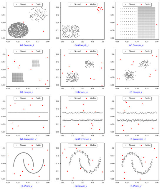
Figure 4. Synthetic data sets for performance evaluation of outlier detection methods.

Table 1. The characteristics of synthetic data sets.

Data Set	Contamination	Number of Instances	Number of Attributes	Number of Outliers
Example_l	0.18%	1100	2	2
Example_c	4.00%	200	2	8
Example_n	0.18%	1100	2	2
Groups, Regressions, and Moons	3.00%	206	2	6
	5.00%	210	2	10
	7.00%	214	2	14

The performance of each detector on the Example_l, Example_c, and Example_n data sets in terms of AUC and PRN is presented in Table 2 and Table 3, respectively. For the Example_l data set, the proposed methods and most algorithms achieve perfect AUC and PRN values of 1.000. whereas ECOD exhibits significant limitations in identifying outliers in this small-scale data set. For the Example_c data set, COF, LoOP, and ECOD achieve the AUC and PRN values consistently lower than average, indicating that these methods fail to accurately detect clustered outliers due to high similarity with normal clusters. For the Example_n data set, LOCI, NOF, and ECOD all fail in this case due to the low local density of the sparse cluster members located near the dense clusters, resulting in normal data being considered outliers. The experiments demonstrate that only the proposed methods and RDOS achieve perfect performance across various scenarios.

Table 2. AUC of various outlier detection methods in Example_l, Example_c, and Example_n data sets.

Data Set	LOF	COF	LoOP	LOCI	NOF	RDOS	ECOD	CCOD	PCOD
Example_l	1.000	1.000	1.000	1.000	1.000	1.000	0.810	1.000	1.000
Example_c	1.000	0.998	0.992	1.000	1.000	1.000	0.998	1.000	1.000
Example_n	1.000	1.000	1.000	0.994	0.988	1.000	0.606	1.000	1.000

Note: Bold values indicate the best performance in each row.

Table 3. PNR of various outlier detection methods in Example_l, Example_c, and Example_n data sets.

Data Set	LOF	COF	LoOP	LOCI	NOF	RDOS	ECOD	CCOD	PCOD
Example_l	1.000	1.000	1.000	1.000	1.000	1.000	0.000	1.000	1.000
Example_c	0.998	0.875	0.625	1.000	1.000	1.000	0.875	1.000	1.000
Example_n	1.000	1.000	1.000	0.500	0.000	1.000	0.500	1.000	1.000

Note: Bold values indicate the best performance in each row.

The performance of each detector on the Groups, Regressions, and Moons data sets in terms of AUC and PRN is presented in Table 4 and Table 5.

Table 4. AUC of various outlier detection methods in Groups, Regressions and Moons data sets.

Data Set		LOF	COF	LoOP	LOCI	NOF	RDOS	ECOD	CCOD	PCOD
Groups_e	$3\%$	1.000	1.000	1.000	1.000	1.000	1.000	0.722	1.000	1.000
	$5\%$	1.000	1.000	1.000	1.000	1.000	1.000	0.762	1.000	1.000
	$7\%$	0.978	0.929	0.948	0.974	0.956	0.986	0.781	0.964	0.994
Groups_u	$3\%$	1.000	1.000	1.000	1.000	0.994	1.000	0.782	1.000	1.000
	$5\%$	1.000	1.000	1.000	1.000	0.999	1.000	0.827	1.000	1.000
	$7\%$	1.000	1.000	1.000	1.000	0.994	1.000	0.840	1.000	1.000
Groups_g	$3\%$	1.000	1.000	1.000	1.000	1.000	1.000	0.830	1.000	1.000
	$5\%$	0.980	1.000	0.998	1.000	0.997	1.000	0.871	0.982	0.987
	$7\%$	0.929	0.996	0.995	0.998	0.989	1.000	0.806	0.918	0.897
Regressions_e	$3\%$	0.999	1.000	0.999	0.967	0.906	0.999	0.949	0.985	1.000
	$5\%$	1.000	1.000	1.000	1.000	1.000	1.000	0.964	1.000	1.000
	$7\%$	1.000	1.000	1.000	1.000	1.000	1.000	0.950	1.000	1.000
Regressions_u	$3\%$	0.998	1.000	0.998	0.944	0.827	0.998	0.951	1.000	1.000
	$5\%$	1.000	1.000	1.000	1.000	1.000	1.000	0.949	1.000	1.000
	$7\%$	0.992	1.000	0.999	0.977	0.934	0.999	0.917	0.985	1.000
Regressions_g	$3\%$	0.990	0.997	0.999	0.998	0.992	0.999	0.971	0.958	0.968
	$5\%$	0.989	0.998	0.999	0.999	0.995	1.000	0.960	0.989	0.981
	$7\%$	0.936	0.998	0.998	0.999	0.965	0.999	0.939	0.953	0.886
Moons_e	$3\%$	1.000	1.000	1.000	0.977	0.965	1.000	0.673	1.000	1.000
	$5\%$	1.000	0.990	1.000	0.988	0.975	1.000	0.768	1.000	1.000
	$7\%$	1.000	0.950	0.999	0.991	0.924	0.949	0.753	1.000	0.919
Moons_u	$3\%$	1.000	1.000	1.000	1.000	0.998	1.000	0.645	1.000	1.000
	$5\%$	0.999	0.999	1.000	0.996	0.984	1.000	0.737	1.000	1.000
	$7\%$	0.998	0.998	0.999	0.997	0.978	0.994	0.675	0.964	0.980
Moons_g	$3\%$	0.899	1.000	1.000	0.982	0.879	0.999	0.693	1.000	0.999
	$5\%$	0.895	0.999	0.999	0.989	0.899	0.999	0.805	0.999	0.740
	$7\%$	0.939	0.999	0.999	0.994	0.949	0.998	0.765	0.980	0.699

Note: Bold values indicate the best performance in each row.

Table 5. PNR of various outlier detection methods in synthetic data sets.

Data Set		LOF	COF	LoOP	LOCI	NOF	RDOS	ECOD	CCOD	PCOD
Groups_e	$3\%$	1.000	1.000	1.000	1.000	1.000	1.000	0.500	1.000	1.000
	$5\%$	1.000	1.000	1.000	1.000	1.000	1.000	0.600	1.000	1.000
	$7\%$	0.929	0.929	0.929	0.929	0.929	0.929	0.571	1.000	1.000
Groups_u	$3\%$	1.000	1.000	1.000	1.000	0.833	1.000	0.333	1.000	1.000
	$5\%$	1.000	1.000	1.000	1.000	0.900	1.000	0.500	1.000	1.000
	$7\%$	1.000	1.000	1.000	1.000	0.929	1.000	0.500	1.000	1.000
Groups_g	$3\%$	1.000	1.000	1.000	1.000	1.000	1.000	0.667	1.000	1.000
	$5\%$	0.955	0.989	0.900	1.000	0.967	1.000	0.500	0.893	0.980
	$7\%$	0.903	0.905	0.881	0.929	0.881	0.976	0.571	0.785	0.818
Regressions_e	$3\%$	0.800	1.000	0.900	0.900	0.800	0.900	0.667	0.973	1.000
	$5\%$	1.000	1.000	1.000	1.000	1.000	1.000	0.800	1.000	1.000
	$7\%$	1.000	1.000	1.000	1.000	1.000	1.000	0.643	1.000	1.000
Regressions_u	$3\%$	0.833	1.000	0.833	0.833	0.667	0.833	0.333	1.000	1.000
	$5\%$	1.000	1.000	1.000	1.000	1.000	1.000	0.300	1.000	1.000
	$7\%$	0.857	1.000	0.929	0.929	0.857	0.929	0.429	0.791	1.000
Regressions_g	$3\%$	0.889	0.889	0.889	0.944	0.889	0.944	0.333	0.894	0.792
	$5\%$	0.967	0.933	0.967	0.967	0.900	0.967	0.500	0.967	0.917
	$7\%$	0.926	0.929	0.929	0.953	0.857	0.905	0.500	0.944	0.864
Moons_e	$3\%$	1.000	1.000	1.000	0.833	0.667	1.000	0.333	1.000	1.000
	$5\%$	1.000	0.867	1.000	0.900	0.700	1.000	0.600	1.000	1.000
	$7\%$	1.000	0.929	0.929	0.929	0.714	0.929	0.500	1.000	0.750
Moons_u	$3\%$	1.000	1.000	1.000	1.000	0.833	1.000	0.167	1.000	1.000
	$5\%$	0.900	0.900	1.000	0.900	0.800	0.900	0.400	1.000	1.000
	$7\%$	0.929	0.857	0.857	0.929	0.714	0.857	0.286	1.000	0.636
Moons_g	$3\%$	0.744	0.944	0.944	0.944	0.722	0.889	0.333	1.000	0.944
	$5\%$	0.833	0.933	0.900	0.933	0.733	0.900	0.400	0.933	0.740
	$7\%$	0.640	0.953	0.929	0.929	0.786	0.929	0.500	0.833	0.729

Note: Bold values indicate the best performance in each row.

For the Groups data sets, most methods achieve perfect AUC and PRN values of $1.000$ on Group_e and Group_u when the contamination is $3\%$ and $5\%$, except for NOF and ECOD. However, as the contamination increases to $7\%$, only CCOD and PCOD maintain perfect AUC and PRN values of $1.000$ on Group_u, while on Group_e, PCOD achieves the highest AUC of $0.994$. Particularly, on Group_e with $7\%$ contamination, PCOD outperforms LOF, COF, LoOP, LOCI, NOF, RDOS, and ECOD by $0.016$, $0.065$, $0.046$, $0.020$, $0.038$, $0.008$, and $0.213$, respectively. For the more irregular Group_g data set with $7\%$ contamination, CCOD achieves an AUC of $0.918$ and PRN of $0.785$, while PCOD obtains an AUC of $0.897$ and PRN of $0.818$, demonstrating CCOD’s superior sensitivity to local distribution variations in terms of AUC.

On the Regressions data sets, LOF, LoOP, LOCI, and RDOS show relatively unstable AUC values and correspondingly lower PRN values on linearly distributed data, while COF consistently demonstrates strong performance through its shortest-path linkage mechanism. Specifically, under $3\%$ contamination in Regression_e, LOF and NOF achieve PRN values of only $0.800$, ECOD obtains $0.667$, whereas CCOD reaches $0.973$. When the contamination increases to $5\%$, CCOD and PCOD both achieve perfect scores with AUC and PRN of $1.000$ on Regression_e and Regression_u, indicating that the chaining theory effectively adapts to linear manifold structures. However, at $5\%$ contamination on the Gaussian-distributed Regression_g, the performance of both methods degrades to AUC values of $0.989$ and $0.981$, with corresponding PRN values of $0.967$ and $0.917$, respectively, suggesting room for improvement in scenarios with more complex density distributions.

For the Moons data sets, most methods show significant performance degradation due to difficulties in capturing the diverse data distribution structures. CCOD and PCOD maintain perfect AUC and PRN values of $1.000$ across all contamination levels on Moon_e, except that PCOD’s AUC drops to $0.919$ at $7\%$ contamination, and achieve the best AUC and PRN performance at $3\%$ and $5\%$ contaminations on Moon_u and Moon_g. Particularly, on Moon_g with $3\%$ contamination, CCOD outperforms LOF, LOCI, NOF, and ECOD by $0.101$, $0.018$, $0.121$, and $0.307$, respectively. Under $7\%$ contamination on Moon_g, CCOD achieves a PRN of $0.833$ while PCOD obtains $0.729$, demonstrating its superior precision within complex distribution scenarios. The experiments demonstrate the superior robustness of CCOD and PCOD across complex data scenarios with varying contamination levels.

Furthermore, we investigate the parameter tuning and sensitivity analysis for CCOD and PCOD. The minimum cluster size is determined by $\lceil \alpha \times k^2\rceil$, where the parameter $\alpha$ is set to a fixed value of 0.2 in both CCOD and PCOD, whereas $\gamma$ and k are tunable parameters. In the experiments on synthetic data sets, $\gamma$ ranges from 1 to 5 with an interval of 0.2, and k ranges from 5 to 50 with an interval of 5. Empirically, when CCOD and PCOD achieve optimal AUC, the value of $\gamma$ is approximately 3.6. Therefore, we recommend setting $\gamma =3.6$ when prior statistical information is unavailable. Similarly, the optimal value of k is approximately 10 for CCOD and 15 for PCOD. It is recommended that k be increased moderately with growing data set size. Additionally, we evaluate the sensitivity of parameter $\gamma$. As shown in Figure 5, the values of $\gamma$ that achieve optimal AUC in CCOD and PCOD are presented across varying values of k. It is observed that the correlation between $\gamma$ and k is weak, with the variation in $\gamma$ remaining insignificant as k increases from 5 to 50. In Figure 5d, the value of $\gamma$ for both CCOD and PCOD consistently remains at 3.6 across all values of k.

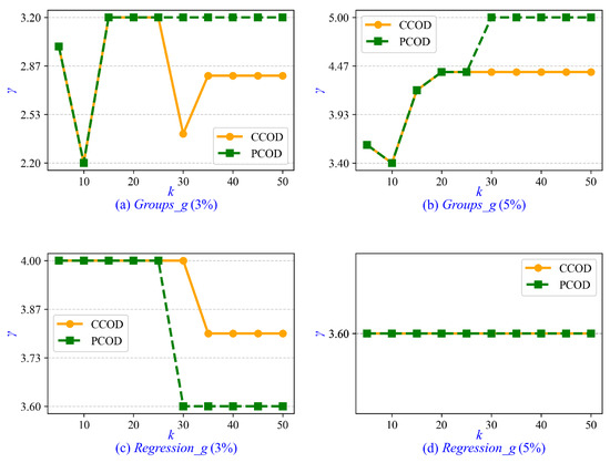
Figure 5. Sensitivity of parameter $\gamma$ to varying k in synthetic data sets.

4.2. Detection Performance on Real-Life Data Sets

To evaluate the predictive performance of different models in real-life scenarios, experiments are conducted on 20 real-life data sets with varying sample sizes, dimensionalities, and contamination. The data sets span diverse applications, including healthcare, sensor readings, handwriting, and tabular benchmarks [40,41]. In the medical domain, the breast cancer Wisconsin data set (abbr., BCancer) contains benign and malignant cases extracted from Fine Needle Aspirate (FNA) images of nuclei. By treating malignant cases as outliers, the performance of the detector is evaluated by identifying malignant cases. In pattern recognition, the pen-based recognition of the handwritten digits data set is a collection of data extracted from digitized handwritten images of different writers. Of these, the Pen-global treats digit 8 as normal and other digits as outliers, and Pen-local treats digit 4 forms an outlier cluster. In remote sensing, the Landsat satellite data set (abbr. Satellite) contains scenes extracted from satellite imagery, where semantic scenes corresponding to cotton crops and soil with vegetation stubble are selected as outliers. All numeric attributes are normalized before being used in our experiments. To mitigate the curse of dimensionality in high-dimensional data sets, we apply principal component analysis for dimensionality reduction while preserving at least 95% of the original variance to maintain detection capability and ensure fair comparison. Table 6 summarizes the comprehensive data set characteristics.

Table 6. The characteristics of real-life data sets.

Data Set	Contamination	Number of Instances	Number of Outliers	Original Dim.	Reduced Dim.
Annthyroid	7.42%	7200	534	6	3
BCancer	2.46%	366	9	30	3
Cardiot	29.73%	2126	632	22	5
Glass	4.21%	214	9	9	5
HeartDis	45.87%	303	139	14	3
Hepatitis	20.65%	155	32	20	3
Ionosphere	35.90%	351	126	33	24
Letter	6.25%	1599	100	32	19
Musk	3.17%	3062	97	166	27
Optdigits	2.88%	5216	150	64	29
Page_blocks	10.23%	5473	560	11	3
Pendigits	2.27%	6870	156	16	9
Pen-global	11.14%	808	90	16	9
Pen-local	0.15%	6723	10	16	9
Satellite	1.45%	5099	74	36	6
Shuttle	1.89%	46,463	878	9	3
Spambase	39.40%	4601	1813	58	3
Vowels	3.43%	1456	50	12	8
Waveform	2.90%	3443	100	22	19
Wine	7.75%	129	10	13	3

Table 7 and Table 8 present the AUC and PRN performance of each detector on 20 real-life data sets, with rankings shown in parentheses. Overall, PCOD achieves the highest average AUC of $0.71$, while CCOD attains the highest average PRN of $0.46$ and the second-best AUC of $0.69$.

Table 7. AUC of various outlier detection methods in real-life data sets.

Data Set	LOF	COF	LoOP	LOCI	NOF	RDOS	ECOD	CCOD	PCOD
Annthyroid	0.62(4)	0.63(3)	0.62(4)	0.61(7)	0.62(4)	0.60(8)	0.60(8)	0.64(2)	0.66(1)
BCancer	0.83(1)	0.77(5)	0.77(5)	0.77(5)	0.60(9)	0.79(3)	0.66(8)	0.79(3)	0.83(1)
Cardiot	0.60(3)	0.58(6)	0.61(1)	0.60(3)	0.50(8)	0.53(7)	0.50(8)	0.59(5)	0.61(1)
Glass	0.70(1)	0.68(3)	0.66(6)	0.68(3)	0.60(8)	0.63(7)	0.58(9)	0.67(5)	0.69(2)
HeartDis	0.62(5)	0.64(2)	0.62(5)	0.63(3)	0.51(9)	0.55(8)	0.56(7)	0.63(3)	0.65(1)
Hepatitis	0.61(4)	0.64(1)	0.60(6)	0.61(4)	0.52(8)	0.55(7)	0.50(9)	0.62(3)	0.64(1)
Ionosphere	0.68(4)	0.68(4)	0.68(4)	0.69(3)	0.60(9)	0.65(7)	0.61(8)	0.71(2)	0.72(1)
Letter	0.70(2)	0.70(2)	0.72(1)	0.65(6)	0.48(9)	0.57(8)	0.58(7)	0.70(2)	0.70(2)
Musk	0.60(6)	0.63(4)	0.65(3)	0.61(5)	0.55(7)	0.52(9)	0.53(8)	0.74(2)	0.76(1)
Optdigits	0.58(5)	0.60(3)	0.59(4)	0.58(5)	0.53(7)	0.50(8)	0.50(8)	0.67(2)	0.69(1)
Page_blocks	0.68(1)	0.65(5)	0.66(3)	0.64(6)	0.60(7)	0.59(8)	0.58(9)	0.66(3)	0.67(2)
Pen-global	0.76(4)	0.82(2)	0.71(6)	0.58(8)	0.57(9)	0.70(7)	0.76(4)	0.82(2)	0.84(1)
Pen-local	0.56(5)	0.65(3)	0.55(6)	0.51(8)	0.51(8)	0.58(4)	0.55(6)	0.73(1)	0.71(2)
Pendigits	0.60(5)	0.58(6)	0.62(4)	0.63(3)	0.55(8)	0.56(7)	0.50(9)	0.65(2)	0.67(1)
Satellite	0.78(3)	0.77(4)	0.72(6)	0.62(9)	0.75(5)	0.69(7)	0.68(8)	0.79(2)	0.84(1)
Shuttle	0.62(4)	0.62(4)	0.63(2)	0.61(6)	0.57(8)	0.55(9)	0.60(7)	0.63(2)	0.65(1)
Spambase	0.58(4)	0.58(4)	0.56(6)	0.55(7)	0.50(9)	0.52(8)	0.61(3)	0.65(2)	0.67(1)
Vowels	0.62(6)	0.68(1)	0.64(4)	0.63(5)	0.58(8)	0.59(7)	0.54(9)	0.66(3)	0.67(2)
Waveform	0.64(3)	0.65(2)	0.60(6)	0.61(5)	0.55(7)	0.55(7)	0.54(9)	0.64(3)	0.66(1)
Wine	0.80(6)	0.80(6)	0.82(3)	0.81(4)	0.78(8)	0.84(1)	0.60(9)	0.81(4)	0.84(1)
Avg.	0.66(4)	0.67(3)	0.65(5)	0.63(6)	0.57(9)	0.60(7)	0.58(8)	0.69(2)	0.71(1)

Note: Bold values indicate the best performance in each row.

Table 8. PNR of various outlier detection methods in real-life data sets.

Data Set	LOF	COF	LoOP	LOCI	NOF	RDOS	ECOD	CCOD	PCOD
Annthyroid	0.28(4)	0.30(3)	0.28(4)	0.25(7)	0.28(4)	0.24(8)	0.23(9)	0.35(1)	0.35(1)
BCancer	0.67(1)	0.56(4)	0.56(4)	0.56(4)	0.22(9)	0.44(7)	0.33(8)	0.67(1)	0.67(1)
Cardiot	0.41(3)	0.40(6)	0.42(1)	0.41(3)	0.36(8)	0.38(7)	0.36(8)	0.41(3)	0.42(1)
Glass	0.36(1)	0.35(3)	0.34(6)	0.35(3)	0.31(8)	0.33(7)	0.30(9)	0.35(3)	0.36(1)
HeartDis	0.46(3)	0.46(3)	0.44(5)	0.33(8)	0.26(9)	0.37(6)	0.36(7)	0.53(1)	0.50(2)
Hepatitis	0.46(3)	0.46(3)	0.43(5)	0.32(8)	0.27(9)	0.37(6)	0.33(7)	0.52(1)	0.49(2)
Ionosphere	0.50(3)	0.48(4)	0.47(5)	0.35(8)	0.29(9)	0.42(6)	0.38(7)	0.58(1)	0.54(2)
Letter	0.44(2)	0.44(2)	0.47(1)	0.34(6)	0.02(9)	0.27(7)	0.21(8)	0.44(2)	0.44(2)
Musk	0.31(6)	0.33(4)	0.34(3)	0.32(5)	0.29(7)	0.27(9)	0.28(8)	0.38(2)	0.39(1)
Optdigits	0.40(5)	0.41(3)	0.41(3)	0.40(5)	0.38(7)	0.36(8)	0.36(8)	0.45(2)	0.46(1)
Page_blocks	0.35(1)	0.34(3)	0.34(3)	0.33(6)	0.31(7)	0.31(7)	0.30(9)	0.34(3)	0.35(1)
Pen-global	0.57(5)	0.68(2)	0.49(6)	0.24(8)	0.23(9)	0.49(6)	0.58(4)	0.66(3)	0.70(1)
Pen-local	0.11(5)	0.22(4)	0.11(5)	0.00(8)	0.00(8)	0.29(3)	0.11(5)	0.60(1)	0.60(1)
Pendigits	0.31(5)	0.30(6)	0.32(4)	0.33(3)	0.29(7)	0.29(7)	0.26(9)	0.34(2)	0.35(1)
Satellite	0.57(1)	0.54(2)	0.45(5)	0.26(9)	0.51(3)	0.39(6)	0.32(7)	0.51(3)	0.30(8)
Shuttle	0.32(4)	0.32(4)	0.33(2)	0.32(4)	0.30(8)	0.29(9)	0.31(7)	0.33(2)	0.34(1)
Spambase	0.44(3)	0.42(4)	0.41(5)	0.30(9)	0.36(7)	0.36(7)	0.38(6)	0.55(1)	0.52(2)
Vowels	0.46(4)	0.48(3)	0.45(5)	0.33(8)	0.28(9)	0.39(6)	0.35(7)	0.50(2)	0.53(1)
Waveform	0.33(3)	0.34(1)	0.31(6)	0.32(5)	0.29(7)	0.29(7)	0.28(9)	0.33(3)	0.34(1)
Wine	0.42(4)	0.42(4)	0.43(3)	0.42(4)	0.41(8)	0.44(1)	0.31(9)	0.42(4)	0.44(1)
Avg.	0.41(3)	0.41(3)	0.39(5)	0.32(7)	0.28(9)	0.35(6)	0.32(7)	0.46(1)	0.45(2)

Note: Bold values indicate the best performance in each row.

For low contamination data sets (≤5%), we analyze 10 data sets with contamination ranging from $0.15\%$ to $4.21\%$. In this case, PCOD demonstrates exceptional performance, achieving first rank in 7 out of 10 data sets, while CCOD consistently delivers competitive results. For the BCancer data set, PCOD and LOF achieve the highest AUC of $0.83$ with a PRN of $0.67$, surpassing COF, LoOP, and LOCI by $0.06$, NOF by $0.23$, RDOS by $0.04$, and ECOD by $0.17$. For the Musk data set, PCOD achieves the best performance with an AUC of $0.76$ and PRN of $0.39$, significantly outperforming LOF by $0.16$. For the Pen-local data set, both CCOD and PCOD achieve a PRN of $0.60$, while CCOD achieves the highest AUC of $0.73$ compared to PCOD’s $0.71$, benefiting from its more refined cascaded local search mechanism that effectively identifies small outlier clusters. For the Shuttle and Optdigits data sets, PCOD achieves the highest AUC, and CCOD is the second highest performer. The superior performance is particularly notable on large-scale data sets, where PCOD achieves substantial improvements over other methods.

For medium contamination data sets (5–20%), we evaluate 5 data sets with contamination between $6.25\%$ and $11.14\%$. In this case, PCOD ranks first in 3 out of 5 data sets, while CCOD consistently ranks in the top-4 across these data sets. For the Annthyroid data set, PCOD achieves the best performance with an AUC of $0.66$ and PRN of $0.35$, its AUC outperforms LOF by $0.04$, and significantly surpasses NOF and ECOD by $0.06$. For the Pen-global data set, PCOD achieves the highest AUC of $0.84$, demonstrating superior effectiveness over LOCI by $0.26$ and NOF by $0.27$, showcasing excellent performance in pattern recognition tasks such as handwriting recognition. However, on the Letter data set, LoOP achieves the highest AUC of $0.72$, with PCOD and CCOD at $0.70$. This occurs because traditional methods can use exact contamination levels as prior knowledge, whereas CCOD and PCOD determine outliers based on chaining distances without prior contamination knowledge, which may reduce precision in some cases.

For high contamination data sets ($\ge 20\%$), we test 5 challenging data sets with contamination from $20.65\%$ to $45.87\%$. Despite the challenging conditions with dense outlier distributions, PCOD maintains first ranking in all 5 data sets, while CCOD maintains competitive performance. For the HeartDis data set with the highest contamination ($45.87\%$), PCOD achieves the best AUC of $0.65$ and CCOD achieves $0.63$, with PCOD obtaining a PRN of $0.50$ and CCOD achieving a PRN of $0.53$, demonstrating strong performance. For the Spambase data set, PCOD attains the highest AUC of $0.67$ with a PRN of $0.52$, with CCOD achieving the second-best AUC of $0.65$ and a PRN of $0.55$, substantially outperforming traditional methods like LOF and COF. In contrast, traditional methods show significant performance degradation in high contamination scenarios. For instance, ECOD achieves only $0.60$ AUC with a PRN of $0.31$ on the Wine data set, while NOF obtains AUC values below $0.55$ with PRN values generally below $0.40$ on multiple high contamination data sets. Although COF and LOF maintain competitiveness on some data sets, their overall performance remains unstable. The ensemble method ECOD demonstrates poor performance on multiple data sets, highlighting the limitations of feature independence assumptions. In this case, contamination parameters have a significant impact on outlier detection performance, and even minor contamination variations can cause significant changes in results. However, the proposed methods remain effective when dealing with highly contaminated data.

We present the running time analysis on real-life data sets. Detectors ranked by average execution time are: ECOD (1.73s), LOF (1.80s), PCOD (2.68s), NOF (2.82s), CCOD (3.95s), RDOS (7.27s), LOCI (23.97s), LoOP (39.27s), and COF (51.67s). ECOD achieves linear complexity $\mathrm{O}\left(n\right)$, while LOCI has cubic complexity $\mathrm{O}\left(n^3\right)$. Other methods, including LOF, NOF, RDOS, LoOP, COF, and the proposed CCOD and PCOD, have quadratic complexity $\mathrm{O}\left(n^2\right)$. Among the $\mathrm{O}\left(n^2\right)$ methods, LOF is computationally the most efficient, involving only distance calculations and simple density ratios. In contrast, NOF requires bidirectional verification of mutual k-nearest neighbors, RDOS and LoOP incur overhead from kernel density estimation and probabilistic computations, and COF suffers from expensive shortest path construction across connectivity patterns. Our CCOD and PCOD methods achieve practical efficiency comparable to LOF through streamlined contrastive computations, while delivering superior detection accuracy, effectively balancing cost and performance.

Experimental results demonstrate that our chain-based approaches consistently outperform state-of-the-art methods across both synthetic and real-life data sets, validating the effectiveness of chain-based theory in tackling complex outlier detection scenarios.

Furthermore, we investigate the parameter tuning and sensitivity analysis for CCOD and PCOD. The minimum cluster size is determined by $\lceil \alpha \times k^2\rceil$, where the parameter $\alpha$ is set to a fixed value of 0.2 in both CCOD and PCOD, whereas $\gamma$ and k are tunable parameters. In the experiments on real-life data sets, $\gamma$ ranges from 1 to 5 with an interval of 0.2, and k ranges from 5 to 50 with an interval of 5. Empirically, when CCOD and PCOD achieve optimal AUC, the value of $\gamma$ is approximately 3.6. Therefore, we recommend setting $\gamma =3.6$ when prior statistical information is unavailable. Similarly, the optimal value of k is approximately 15 for CCOD and 25 for PCOD. It is recommended that k be increased moderately with growing data set size. Additionally, we evaluate the sensitivity of parameter $\gamma$. As shown in Figure 6, the values of $\gamma$ that achieve optimal AUC in CCOD and PCOD are presented across varying values of k. It is observed that the correlation between $\gamma$ and k is weak, with the variation in $\gamma$ remaining insignificant as k increases from 5 to 50. In Figure 6b, the value of $\gamma$ for both CCOD and PCOD consistently remains at 3.6 across all values of k.

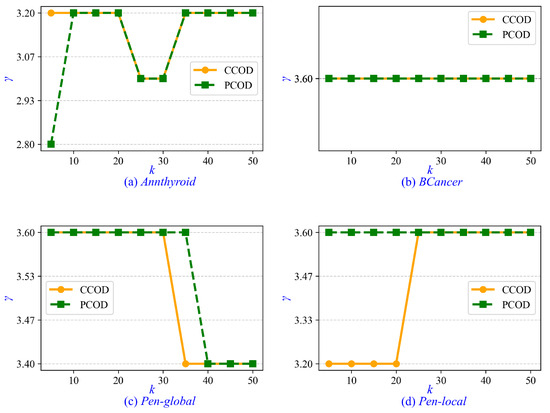
Figure 6. Sensitivity of parameter $\gamma$ to varying k in real-life data sets.

5. Conclusions

This paper proposes a novel chain-based theory for outlier detection that simultaneously addresses multiple challenges in complex data scenarios: handling different outlier types, adapting to varying cluster densities, and eliminating dependence on contamination parameters. We present CCOD and PCOD, two interpretable methods that utilize chaining distance as a manifold-aware data distribution estimator, identifying outliers through sudden distance increases in geodesic connectivity paths while providing intuitive explanations for detection decisions. Through extensive experiments with both synthetic data sets and real-life data sets, we demonstrate that performance is comparable or better to state-of-the-art methods, establishing chain-based theory as a promising solution for addressing complex data scenarios in outlier detection. The contamination-free design and computational efficiency make these methods particularly suitable for intelligent O&M applications where outlier proportions are unknown and large-scale monitoring is required. These results establish chain-based theory as a promising solution for addressing complex data scenarios in outlier detection.

Future work will extend our approach to real-time applications by developing online learning capabilities that can adapt to evolving operational conditions and integrate with existing maintenance decision support systems. We also aim to validate our methods across diverse transportation equipment types and develop comprehensive multi-modal sensor fusion frameworks that can provide holistic fault diagnosis for complex mechanical systems in dynamic operational environments.

References

- Yao, Y.; Zhang, X.; Cui, W. A LOF-IDW based data cleaning method for quality assessment in intelligent compaction of soils. Transp. Geotech. 2023, 42, 101101. [Google Scholar] [CrossRef]
- Bałdyga, M.; Barański, K.; Belter, J.; Origlia, R.; Rossi, B. Anomaly detection in railway sensor data environments: State-of-the-art methods and empirical performance evaluation. Sensors 2024, 24, 2633. [Google Scholar] [CrossRef] [PubMed]
- Bianchi, G.; Fanelli, C.; Freddi, F.; Giuliani, F.; La Placa, A. Systematic review railway infrastructure monitoring: From classic techniques to predictive maintenance. Adv. Mech. Eng. 2025, 17, 16878132241285631. [Google Scholar] [CrossRef]
- Xing, Z.; Liu, Y.; Wang, Q.; Li, J. Multi-sensor signals with parallel attention convolutional neural network for bearing fault diagnosis. AIP Adv. 2022, 12, 075020. [Google Scholar] [CrossRef]
- Wang, X.; Mao, D.; Li, X. Bearing fault diagnosis based on vibro-acoustic data fusion and 1D-CNN network. Measurement 2021, 173, 108518. [Google Scholar] [CrossRef]
- Li, X.; Wang, Y.; Yao, J.; Zhang, H. Multi-sensor fusion fault diagnosis method of wind turbine bearing based on adaptive convergent viewable neural networks. Reliab. Eng. Syst. Saf. 2024, 245, 109980. [Google Scholar] [CrossRef]
- Wan, H.; Gu, X.; Yang, S.; Liu, P. A sound and vibration fusion method for fault diagnosis of rolling bearings under speed-varying conditions. Sensors 2023, 23, 3130. [Google Scholar] [CrossRef]
- Pacheco-Chérrez, J.; Fortoul-Diaz, J.A.; Cortés-Santacruz, F.; Aloso-Valerdi, L.M.; Ibarra-Zarate, D.I. Bearing fault detection with vibration and acoustic signals: Comparison among different machine leaning classification methods. Eng. Fail. Anal. 2022, 139, 106515. [Google Scholar] [CrossRef]
- Chen, S.; Wang, W.; van Zuylen, H. A comparison of outlier detection algorithms for ITS data. Expert Syst. Appl. 2010, 37, 1169–1178. [Google Scholar] [CrossRef]
- Ribeiro, R.P.; Pereira, P.; Gama, J. Sequential anomalies: A study in the railway industry. Mach. Learn. 2016, 105, 127–153. [Google Scholar] [CrossRef]
- Ghiasi, R.; Khan, M.A.; Sorrentino, D.; Friswell, M.I. An unsupervised anomaly detection framework for onboard monitoring of railway track geometrical defects using one-class support vector machine. Eng. Appl. Artif. Intell. 2024, 133, 108167. [Google Scholar] [CrossRef]
- Wan, T.H.; Tsang, C.W.; Hui, K.; Ho, I.W.H. Anomaly detection of train wheels utilizing short-time Fourier transform and unsupervised learning algorithms. Eng. Appl. Artif. Intell. 2023, 122, 106037. [Google Scholar] [CrossRef]
- Phusakulkajorn, W.; Núñez, A.; Wang, H.; Dollevoet, R. Artificial intelligence in railway infrastructure: Current research, challenges, and future opportunities. Intell. Transp. Infrastruct. 2023, 2, liad016. [Google Scholar] [CrossRef]
- Shaikh, M.Z.; Jatoi, S.; Baro, E.N.; Ahmed, A.; Memon, T.D. FaultSeg: A Dataset for Train Wheel Defect Detection. Sci. Data 2025, 12, 309. [Google Scholar] [CrossRef]
- Liu, H.; Zhang, S.; Wu, Z. Outlier detection using local density and global structure. Pattern Recognit. 2025, 157, 110947. [Google Scholar] [CrossRef]
- Omar, M.; Sukthankar, G. Text-Defend: Detecting Adversarial Examples using Local Outlier Factor. In Proceedings of the IEEE International Conference on Semantic Computing, Laguna Hills, CA, USA, 27 February–1 March 2023; pp. 118–122. [Google Scholar]
- Ruff, L.; Kauffmann, J.R.; Vandermeulen, R.A.; Montavon, G.; Samek, W.; Kloft, M.; Dietterich, T.G.; Müller, K.R. A unifying review of deep and shallow anomaly detection. Proc. IEEE 2021, 109, 756–795. [Google Scholar] [CrossRef]
- Liu, B.; Tan, P.N.; Zhou, J. Unsupervised anomaly detection by robust density estimation. In Proceedings of the AAAI Conference on Artificial Intelligence, Virtually, 22 February–1 March 2022; Volume 36, pp. 4101–4108. [Google Scholar]
- Romano, M.; Faiella, G.; Bifulco, P.; Cesarelli, M. Outliers detection and processing in CTG monitoring. In XIV Mediterranean Conference on Medical and Biological Engineering and Computing 2016; Springer: Cham, Switzerland, 2014; pp. 651–654. [Google Scholar]
- Perini, L.; Bürkner, P.C.; Klami, A. Estimating the contamination factor’s distribution in unsupervised anomaly detection. In Proceedings of the 40th International Conference on Machine Learning, Honolulu, HI, USA, 23–29 July 2023; pp. 27668–27679. [Google Scholar]
- Pearson, R.K. Outliers in process modeling and identification. IEEE Trans. Control Syst. Technol. 2002, 10, 55–63. [Google Scholar] [CrossRef]
- Dong, H.; Wang, Q.G.; Ding, W. Chain-Based Outlier Detection for Complex Data Scenarios. In Proceedings of the 2023 IEEE International Conference on Big Data (BigData), Sorrento, Italy, 15–18 December 2023; pp. 504–509. [Google Scholar]
- Yang, J.; Zhou, K.; Li, Y.; Liu, Z. Generalized out-of-distribution detection: A survey. Int. J. Comput. Vis. 2024, 132, 5635–5662. [Google Scholar] [CrossRef]
- Breunig, M.M.; Kriegel, H.P.; Ng, R.T.; Sander, J. LOF: Identifying density-based local outliers. In Proceedings of the 2000 ACM SIGMOD International Conference on Management of Data, Dallas, TX, USA, 16–18 May 2000; pp. 93–104. [Google Scholar]
- Tang, J.; Chen, Z.; Fu, A.W.C.; Cheung, D.W. Enhancing effectiveness of outlier detections for low density patterns. In Advances in Knowledge Discovery and Data Mining; Chen, M.S., Yu, P.S., Liu, B., Eds.; Springer: Berlin/Heidelberg, Germany, 2002; pp. 535–548. [Google Scholar]
- Huang, J.; Zhu, Q.; Yang, L.; Feng, J. A non-parameter outlier detection algorithm based on natural neighbor. Knowl.-Based Syst. 2016, 92, 71–77. [Google Scholar] [CrossRef]
- Jin, W.; Tung, A.K.H.; Han, J.; Wang, W. Ranking outliers using symmetric neighborhood relationship. In Advances in Knowledge Discovery and Data Mining; Ng, W.K., Kitsuregawa, M., Li, J., Chang, K., Eds.; Springer: Berlin/Heidelberg, Germany, 2006; pp. 577–593. [Google Scholar]
- He, Z.; Xu, X.; Deng, S. Discovering cluster-based local outliers. Pattern Recognit. Lett. 2003, 24, 1641–1650. [Google Scholar] [CrossRef]
- Amer, M.; Goldstein, M. Nearest-neighbor and clustering based anomaly detection algorithms for RapidMiner. In Proceedings of the 3rd RapidMiner Community Meeting and Conference (RCOMM’12), Shenzhen, China, 9–11 May 2012; pp. 1–12. [Google Scholar]
- Ester, M.; Kriegel, H.P.; Sander, J.; Xu, X. A density-based algorithm for discovering clusters in large spatial databases with noise. In Proceedings of the Second International Conference on Knowledge Discovery and Data Mining, Portland, OR, USA, 2–4 August 1996; pp. 226–231. [Google Scholar]
- Campello, R.J.G.B.; Moulavi, D.; Zimek, A.; Sander, J. Hierarchical Density Estimates for Data Clustering, Visualization, and Outlier Detection. ACM Trans. Knowl. Discov. Data 2015, 10, 1–51. [Google Scholar] [CrossRef]
- Du, H.; Zhao, S.; Zhang, D.; Wu, J. Novel clustering-based approach for local outlier detection. In Proceedings of the 2016 IEEE Conference on Computer Communications Workshops (INFOCOM WKSHPS), San Francisco, CA, USA, 10–14 April 2016; pp. 802–811. [Google Scholar]
- Yamanishi, K.; Takeuchi, J.I.; Williams, G.; Milne, P. On-line unsupervised outlier detection using finite mixtures with discounting learning algorithms. In Proceedings of the Seventh ACM SIGKDD International Conference on Knowledge Discovery and Data Mining, San Francisco, CA, USA, 26–29 August 2001; pp. 320–324. [Google Scholar]
- Kriegel, H.P.; Kröger, P.; Schubert, E.; Zimek, A. LoOP: Local outlier probabilities. In Proceedings of the 18th ACM Conference on Information and Knowledge Management, Hong Kong, China, 2–6 November 2009; pp. 1649–1652. [Google Scholar]
- Papadimitriou, S.; Kitagawa, H.; Gibbons, P.B.; Faloutsos, C. LOCI: Fast outlier detection using the local correlation integral. In Proceedings of the 19th International Conference on Data Engineering, Bangalore, India, 5–8 March 2003; pp. 315–326. [Google Scholar]
- Tang, B.; He, H. A local density-based approach for outlier detection. Neurocomputing 2017, 241, 171–180. [Google Scholar] [CrossRef]
- Qin, X.; Cao, L.; Rundensteiner, E.A.; Madden, S. Scalable kernel density estimation-based local outlier detection over large data streams. In Proceedings of the 22nd International Conference on Extending Database Technology (EDBT), Lisbon, Portugal, 26–29 March 2019. [Google Scholar]
- Li, Z.; Zhao, Y.; Botta, N.; Ionescu, C.; Hu, X. COPOD: Copula-Based Outlier Detection. In Proceedings of the 2020 IEEE International Conference on Data Mining (ICDM), Sorrento, Italy, 17–20 November 2020; pp. 1118–1123. [Google Scholar]
- Li, Z.; Zhao, Y.; Hu, X.; Botta, N.; Ionescu, C.; Chen, H.G. ECOD: Unsupervised Outlier Detection Using Empirical Cumulative Distribution Functions. IEEE Trans. Knowl. Data Eng. 2022, 14, 71–77. [Google Scholar] [CrossRef]
- Papers with Code. ODDS (Outlier Detection Data Sets). Available online: https://paperswithcode.com/dataset/odds (accessed on 3 June 2025).
- Campos, G.O.; Zimek, A.; Sander, J.; Campello, R.J.; Micenková, B.; Schubert, E.; Assent, I.; Houle, M.E. On the evaluation of unsupervised outlier detection: Measures, data sets, and an empirical study. Data Min. Knowl. Discov. 2016, 30, 891–927. [Google Scholar] [CrossRef]
Disclaimer/Publisher’s Note: The statements, opinions and data contained in all publications are solely those of the individual author(s) and contributor(s) and not of MDPI and/or the editor(s). MDPI and/or the editor(s) disclaim responsibility for any injury to people or property resulting from any ideas, methods, instructions or products referred to in the content. |
© 2025 by the authors. Licensee MDPI, Basel, Switzerland. This article is an open access article distributed under the terms and conditions of the Creative Commons Attribution (CC BY) license (https://creativecommons.org/licenses/by/4.0/).