1. Introduction
Over the past few decades, economic globalization has reshaped industrial and value chains with unprecedented depth and breadth. While unlocking economies of scale and accelerating technological diffusion, it has also continuously exposed traditional manufacturing to uncertainties such as demand fluctuations and factor price shocks [
1]. As the cornerstone of industrial systems and the macroeconomy, the capacity of the manufacturing sector directly reflects a nation’s comprehensive strength and international competitiveness [
2]. With the advancement of intelligent manufacturing technologies, manufacturing paradigms are shifting from uniformity to diversification, imposing higher demands on enterprises’ production organization and management [
3].
The job shop scheduling problem (JSP) is one of the most fundamental and frequently deliberated decision-making issues in enterprise production management [
4]. Its essence lies in arranging task sequences and allocating resources under limited time and resource constraints, with the aim of minimizing production cycles, reducing costs, and maximizing efficiency [
5]. As a significant extension of JSP, the flexible job shop scheduling problem (FJSP) allows each operation to be processed on multiple alternative machines and enables flexible adjustment of process routes according to task requirements [
6]. This feature not only enhances the flexibility and resource utilization of production systems but also alleviates bottlenecks, enabling enterprises to maintain high production efficiency and delivery reliability even under complex scenarios such as fluctuating order structures and tight due dates [
7]. Consequently, FJSP has become an indispensable tool for modern production scheduling optimization and enterprise operation management, and it has been widely applied in high-demand industries such as semiconductor manufacturing, automotive production, and metallurgical processing [
8].
In real-world production, enterprises under fierce market competition and increasing customer demands are often required to simultaneously shorten production cycles and enhance profits [
9]. However, the production process is frequently accompanied by dynamic events such as job insertions, machine breakdowns, and due date changes, which transform the scheduling problem from a static FJSP into a dynamic FJSP (DFJSP), thereby significantly increasing decision-making complexity [
10]. Moreover, a single optimization objective can no longer meet the needs of modern manufacturing systems, and thus the DFJSP has further evolved into the multi-objective flexible job shop scheduling problem (MODFJSP) [
11].
For the MODFJSP, researchers have proposed various heuristic, metaheuristic, and machine learning approaches [
12,
13,
14]. Although metaheuristic algorithms can effectively cope with uncertainties, they often require re-tuning when applied to new production lines or disturbances, thus limiting their generalization ability [
9]. Deep reinforcement learning (DRL) offers advantages in adaptability and real-time responsiveness, and in particular, multi-agent DRL (MADRL) has demonstrated greater robustness and scalability in solving MODFJSP [
15]. However, existing MADRL-based studies mainly focus on minimizing production time and reducing costs, while placing insufficient emphasis on profit maximization. Especially under uncertain production orders, how to simultaneously ensure production efficiency and maximize net profit remains an urgent challenge. The main contributions of this research are as follows.
For the MODFJSP with dynamic new job arrivals, high-profit urgent jobs, and fluctuating due dates, an optimization model is constructed with two objectives: minimizing makespan and maximizing net profit.
A sequential multi-agent collaborative framework of “job selection → machine assignment” is constructed: the job agent first decides the job to be processed, and the machine agent then assigns the pending operation of the selected job to a feasible machine set, thereby enabling efficient solution of the proposed MODFJSP.
Customized reward functions are designed for the two agents with the objectives of maximizing profit and minimizing makespan, accompanied by adaptive state representations and variable action output mechanisms, which significantly enhance learning efficiency and enable multi-objective collaborative optimization.
The system conducts a comparative analysis of various mainstream DRL algorithms and classical dispatching rules in solving the proposed MODFJSP, thereby identifying the optimal DRL-based solution.
2. Literature Review
In this section, we first review JSP-related studies focusing on cost or profit, then summarize the research contributions on solving FJSP using DRL, and finally highlight the existing research gaps.
2.1. Research on Production Scheduling Problems Considering Cost or Profit
In recent years, an increasing number of researchers have focused on the JSP with energy cost considerations under time-of-use (TOU) electricity pricing, aiming to reduce operating expenses for manufacturing enterprises [
16]. For example, Shen et al. [
17] studied the TOU mechanism by optimizing operation start times, sequencing, and machine assignments, demonstrating that even with a slight increase in makespan, energy costs can be effectively reduced. The study provided a rigorous and practical basis for cost reduction and efficiency improvement in FJSP under TOU pricing. Similarly, Park and ham [
18] incorporated TOU pricing and planned machine downtime to minimize makespan and total energy cost, employing integer linear programming and constraint programming approaches to effectively lower energy consumption in manufacturing.
By contrast, fewer studies have approached scheduling from a profit-oriented perspective, considering the combined impact of scheduling decisions on enterprise revenue and cost. Zouadi et al. [
19] innovatively addressed profit orientation and order acceptance by applying a robust decomposition method to maximize production profit, particularly suitable for industries with volatile prices and fragmented customer demand. In the existing FJSP literature, profit-oriented research remains scarce. However, thanks to the dual flexibility of jobs and machines, FJSP still holds substantial potential for profit improvement. Moreover, the MODFJSP can further embed various dynamic events to achieve global adaptive optimization of production and profit. This study innovatively incorporates enterprise profit into the MODFJSP framework, thereby enhancing the effectiveness of scheduling decisions.
2.2. Research on Solving FJSPs with DRL
With the increasing complexity of scheduling problems and the presence of multiple dynamic disturbances (such as job insertions and price fluctuations), traditional heuristic algorithms can hardly provide efficient responses [
12]. DRL, leveraging its trial-and-error mechanism and adaptive policy learning, offers a new decision-making paradigm for such high-dimensional, dynamic, and non-stationary environments [
20]. In the field of FJSP, an increasing number of researchers have proposed various solutions for FJSP [
21]. For example, Luo [
22] designed a Deep Q-Network (DQN) algorithm to address DFJSP by incorporating new job insertions to reduce delays. Lu et al. [
23] applied a Double Deep Q-Network (DDQN) to solve DFJSP with dynamic job arrivals and urgent job insertions, aiming to minimize makespan (
Cmax) and average tardiness. Lei et al. [
12] proposed a proximal policy optimization (PPO) algorithm with a multi-pointer graph network (MPGN) structure to reduce makespan in FJSP. Existing studies have further verified that when solving FJSP with single-agent DRL methods, the state–action space often suffers from combinatorial explosion, whereas adopting a multi-agent approach can effectively alleviate this issue [
15].
Therefore, multi-agent deep reinforcement learning has been widely applied to solve DFJSP [
24]. For example, Liu et al. [
25] focused on DFJSP with dynamic job arrivals, aiming to minimize total tardiness. Yan et al. [
26] also considered DFJSP with dynamic job arrivals and employed a DQN-based multi-agent framework to address factory selection, job allocation, and operation sequencing, achieving the objective of minimizing total tardiness through agent collaboration. Ref. [
27] proposed a multi-agent deep reinforcement learning based scheduling framework to address the complex scheduling problem in flexible job shops with the integration of automated guided vehicles (AGVs), achieving collaborative optimization of production and transportation resources.
Table 1 summarizes the above studies on applying deep reinforcement learning methods to FJSP, along with our proposed approach.
2.3. Research Gaps
By summarizing the existing studies, three research gaps can be identified:
Most cost- or profit-oriented FJSP studies mainly focus on electricity costs under TOU pricing policies, while giving insufficient attention to the penalty costs incurred by tardiness.
Most studies focus solely on cost; however, in practice, some jobs differ in the remuneration offered by customers due to process complexity or specific requirements. How to incorporate such heterogeneous profits into DFJSP and maximize net profit remains to be further investigated.
Most DRL-based studies on DFJSP primarily consider dynamic events such as new job insertions, while neglecting profit and due date fluctuations. Moreover, when targeting profit maximization and makespan minimization, further technical challenges arise in the design of scheduling strategies and reward functions to improve agent learning efficiency.
3. Problem Description for MODFJSP
In this section, to illustrate the considered MODFJSP, we first provide a detailed description. Next, the notations and constraints are presented. Finally, the mathematical model is formulated.
3.1. Problem Description
The MODFJSP considered in this study can be defined as follows. A set of
n consecutively arriving jobs
J = {1, 2, …,
n} must be processed on
m machines
M = {1, 2, …,
m}. Each job
i consists of
ni operations
Oi = {1, …,
ni}, where
Oi,j denotes the
jth operation of job
i. Each operation
Oi,j can be processed on any machine selected from its predefined feasible machine set
Mi,j (
Mi,j⊆
M). The processing time of operation
Oi,j on machine
k is denoted as
ti,j,k. The arrival time and due date of job
i are denoted as
Ai and
Di, respectively.
Si,j,k and
Ci,j,k represent the actual start time and completion time of operation
Oi,j on machine
k, respectively. The system consists of initial orders and dynamically arriving
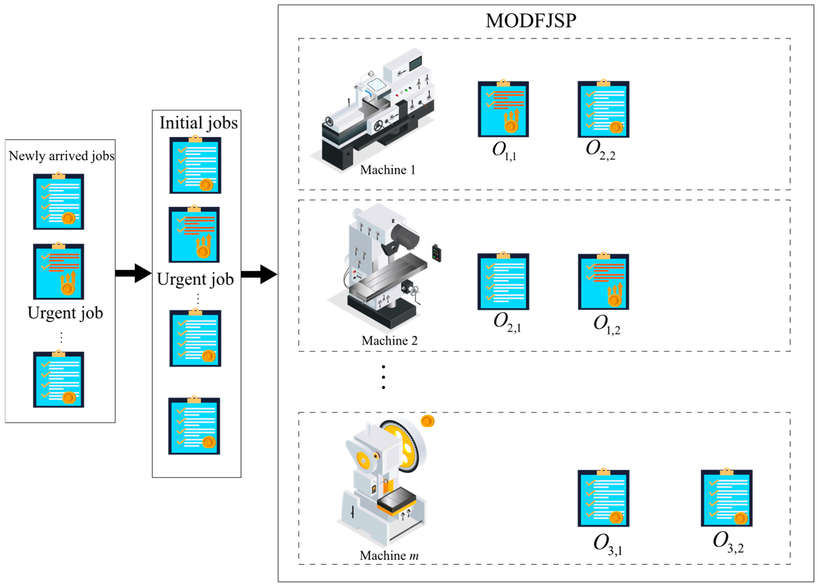
new jobs. Due dates are adjusted according to environmental changes, and some jobs are urgent, generating higher revenue but incurring stricter tardiness penalties. The energy consumption cost is calculated based on TOU electricity pricing. The objectives are to maximize net profit and minimize makespan under resource constraints. The decision process proceeds in two steps: first, selecting the job to be processed, and second, assigning its next operation to a machine. For ease of understanding,
Figure 1 illustrates the considered MODFJSP.
3.2. Mathematical Model
Before presenting the mathematical model of MODFJSP, we provide a detailed description of the notations used.
Table 2 summarizes these notations, including the variables related to jobs, machine resources, processing times, and scheduling decisions.
In real-world production, production efficiency is often reflected in the reduction in
Cmax. Job processing generates electricity consumption costs, while delivery delays incur penalties, which are even higher for urgent orders. Due to differences in process complexity, customer remuneration varies across jobs, and energy consumption also differs among machines. Based on these considerations, this study proposes a bi-objective model aiming to minimize
Cmax and maximize net profit. The objectives and constraints are summarized as follows.
Subject to:
Objective Equation (1) minimizes the
Cmax, while Objective Equation (2) maximizes net profit after accounting for energy costs under TOU pricing and tardiness penalties. Constraint Equation (3) ensures that each job can be processed on at most one machine at any given time. Constraint Equation (4) specifies that if a job is assigned to machine k at time t, then the machine must be in the “on” state at that time. Constraint Equation (5) requires that the completion time of each job be non-negative. Constraint Equation (6) ensures that the processing time of each operation is non-negative. Constraint Equation (7) guarantees that the operations of each job are executed in sequence. Constraint Equation (8) ensures that jobs can only be processed after their arrival time.
4. Multi-Agent Collaboration Framework for the Proposed MODFJSP
Table 3 provides the explanations of the variables and notations used in this section, serving as a reference for the subsequent content. This section first explains the symbols and notations used, then introduces the core algorithms adopted by the multi-agent collaboration framework. Subsequently, it elaborates on the design of each agent’s state inputs, reward functions, and action spaces. Finally, it presents the complete implementation process and technical details for solving the MODFJSP.
4.1. The DRL Algorithm for the Multi-Agent Cooperative Framework
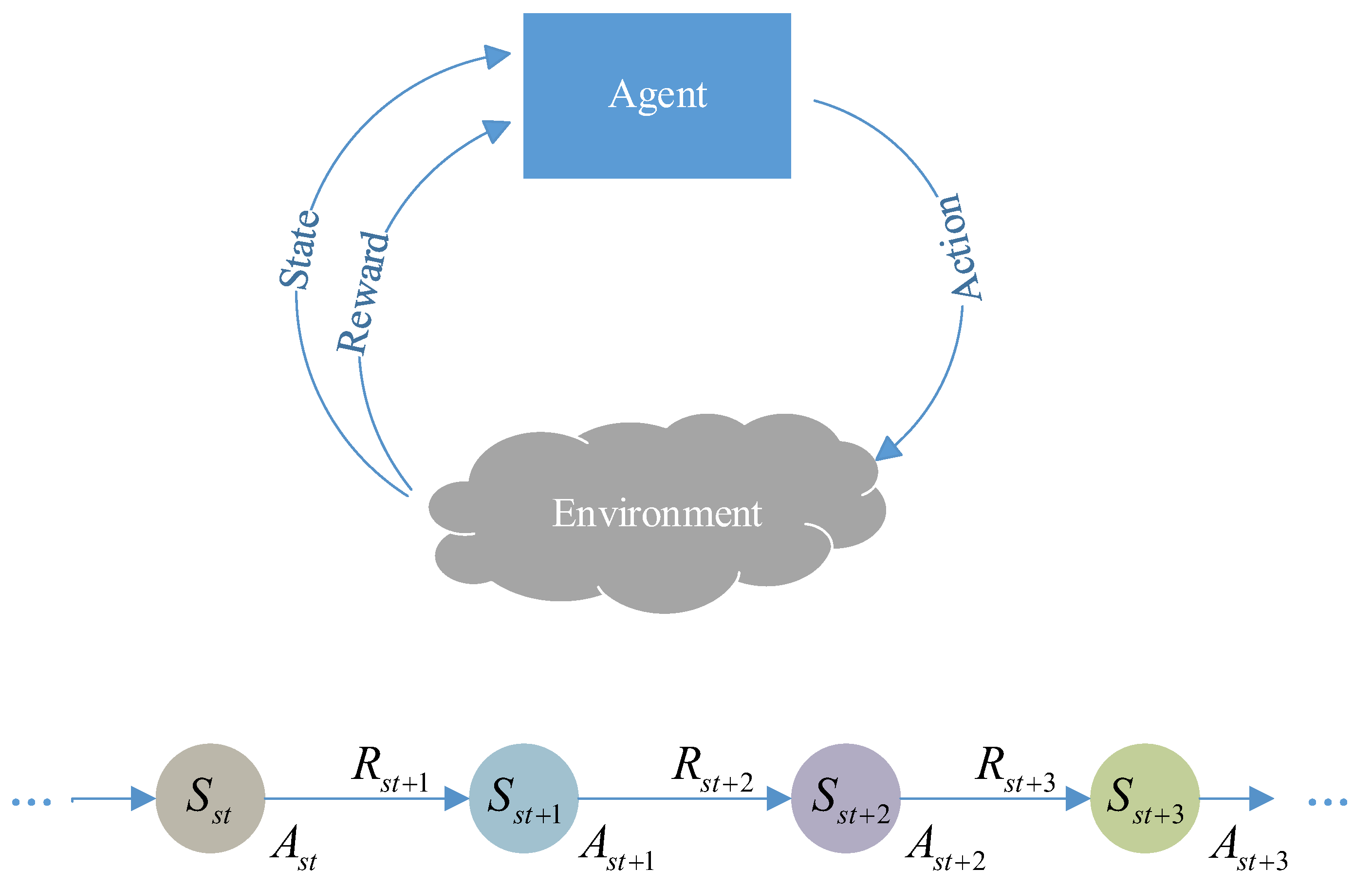
The interaction between reinforcement learning and the scheduling environment is modeled as a Markov Decision Process (MDP) [
28]. MDP is the standard framework for sequential decision-making problems and is typically represented as a four-tuple (S, A, P, R) [
29]. Here, S denotes the state space, A the action space, R the reward function, and P the state transition function.
Figure 2 illustrates the workflow of reinforcement learning (RL) under the MDP framework [
30]. DRL is an extension of RL that integrates deep neural networks into state representation and policy learning. Its main challenge lies in how to stably and efficiently optimize the policy to maximize cumulative rewards, for which various algorithmic strategies (e.g., DQN, DDQN, PPO) have been proposed [
15]. Among them, DDQN is an improvement over DQN designed to alleviate the overestimation of Q-values [
31]. DDQN introduces two networks: the action-selection network (policy network) and the target-evaluation network (target network), thereby decoupling action selection from value estimation [
32]. The target update formula is given as
Here, denotes the parameters of the online network (policy network), and denotes the parameters of the target network. First, the online network is used to select the optimal action at the next decision point st + 1, i.e., . a′ presents candidate action from the action space. Then, the target network evaluates the Q-value of this action.
4.2. Definition of DRL Problem
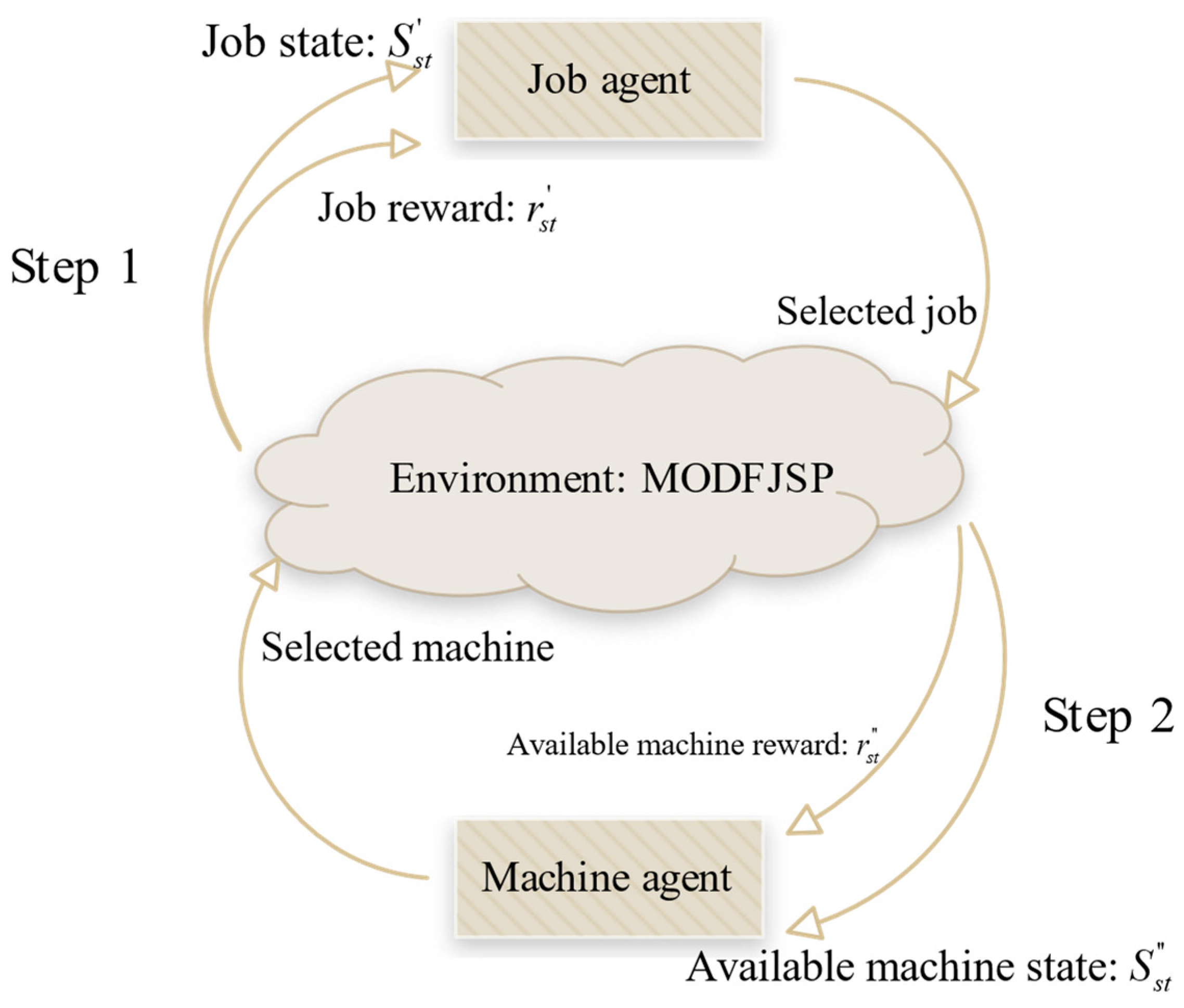
Given the characteristics of FJSP, this study applies DDQN to solve the MOFJSP by employing a new multi-agent framework with a sequential decision-making process: first, the job agent selects the job to be processed and interacts with the MODFJSP environment constructed in this study; then, the environment generates the candidate machine states for the current operation of the selected job; finally, the machine agent chooses an appropriate machine based on this information, forming a “job selection–machine assignment” multi-agent collaborative framework. The overall process is illustrated in
Figure 3, which provides a more intuitive representation of the cooperation between agents.
For the above components, this section sequentially introduces the state inputs, reward functions, and action spaces of the two agents, followed by the detailed procedure of the complete multi-agent solution for MODFJSP.
4.3. State Input
In existing DRL-based studies for solving MODFJSP, the processing status of all jobs is often abstracted into a set of variables [
33], through which agents perceive the shop-floor environment. However, such approaches usually lack fine-grained characterization of unfinished jobs. Based on the characteristics of FJSP and the optimization objectives, this study treats the relevant features of each unfinished job
and its pending operation on each candidate machine
k ∈
Mi,j as variable states, which are then recognized by the job agent and the machine agent. This variable state design enables agents to enhance their decision-making capabilities more effectively.
4.3.1. State Input of the Job Agent
To support the job agent’s decision-making in job selection, the job state
is defined. Each unfinished job state
within it varies with
and can be expressed as
Except for the job index
i, all other features are normalized to enhance the feature discriminability and convergence efficiency of the neural network. A detailed description is provided in
Table 4.
4.3.2. State Input of the Machine Agent
For the selected job
and its pending operation
, the machine agent constructs a state vector for each available machine
:
Table 5 summarizes the detailed descriptions of the available machine state variables.
4.4. Reward Functions
4.4.1. Reward Function of the Job Agent
The job agent takes into account the effects of tardiness and job urgency. If a job is urgent and incurs tardiness, the reward function provides stronger positive guidance while imposing penalties on the degree of tardiness. In this way, under the same conditions, jobs with higher urgency and existing tardiness are prioritized, thereby reducing overall tardiness penalties and improving delivery reliability. Algorithm 1 presents the pseudocode of the reward function.
| Algorithm 1 Reward function of the job agent |
| Input: Selected job , ; |
| Output: |
| 1. | |
| 2. | |
| 3. | = 1 × 10⁻⁶ |
| 4. | if selected job then |
| 5. | + = − |
| 6. | else |
| 7. |
|
| 8. | end if |
| 9. | return |
4.4.2. Reward Function of the Machine Agent
When selecting machines, the machine agent comprehensively considers processing profit, electricity cost, and tardiness impact. First, these three factors are normalized as
, and
, respectively. In the decision-making process, profit is assigned the highest weight, followed by electricity cost from energy consumption, and finally the impact on tardiness. The electricity cost is normalized as the ratio of the actual electricity cost to the benchmark of the “highest electricity price,” where
denotes the maximum unit price in the TOU tariff. Algorithm 2 presents the pseudocode of the reward function for machine selection.
| Algorithm 2 Reward function of the machine agent |
| Input: Selected job ist and machine kst, |
| 1. | |
| 2. | |
| 3. | , is calculated according to Equation (2) |
| 4. | = |
| 5. | |
| 6. | return |
4.5. Definition of Action Spaces
4.5.1. Action Space of the Job Agent
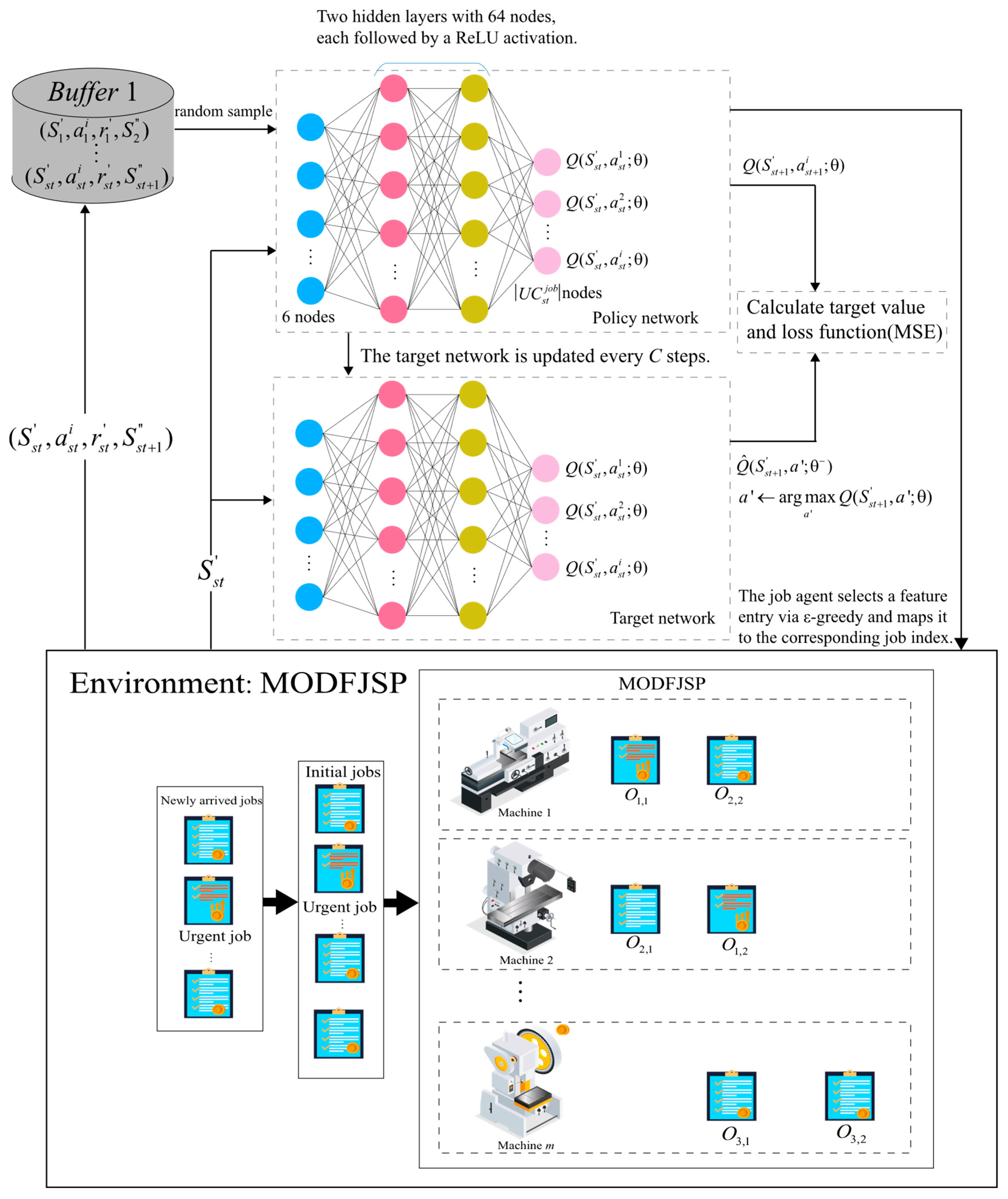
In the decision-making process, the job agent constructs its action space from the states of unfinished jobs, computes the corresponding action values, and then selects the optimal action using the ϵ-greedy strategy. The job index corresponding to the chosen action is the job actually scheduled.
Figure 4 presents the overall structure of the job agent and its interaction process with the environment. At each decision point
st, the job agent first identifies the states of unfinished jobs as input. The policy network outputs
Q-value estimates for all actions, and actions are selected using a greedy strategy. The target network has the same structure as the policy network but is updated differently: the policy network parameters are updated via gradient descent based on the mean squared error (MSE) loss function, while the target network parameters are gradually migrated from the policy network through soft updates, thereby improving training stability and convergence. Meanwhile, DDQN introduces an experience replay mechanism, in which the state transition samples
obtained from environment interactions are stored in a replay buffer. During training, mini-batches of samples are randomly drawn to break data correlations and improve sample efficiency.
4.5.2. Action Space of the Machine Agent
The action space of the machine agent is composed of the set of state feature vectors of all candidate machines capable of processing the job.
The machine agent computes the corresponding action values based on the given features and selects the optimal action using the ϵ-greedy strategy. The machine index corresponding to the chosen action is then assigned as the processing machine for
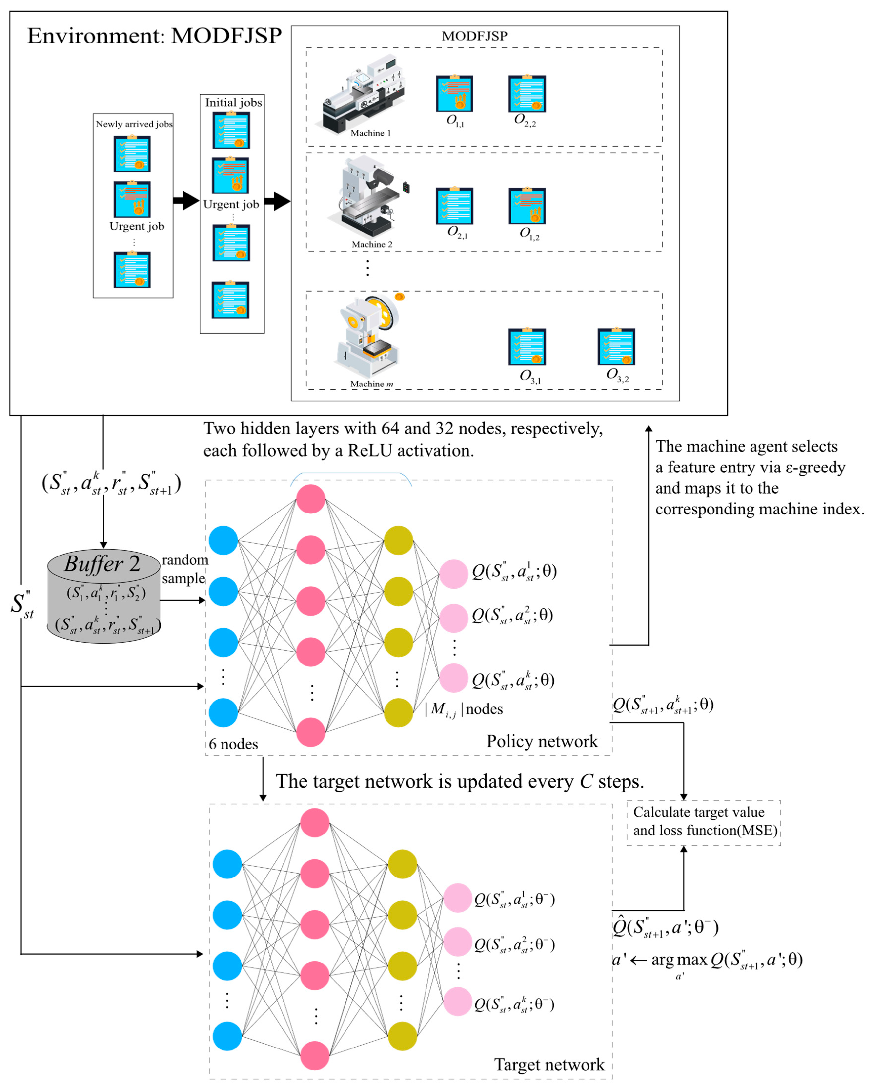
The network structure of the machine agent is illustrated in
Figure 5. At each scheduling point
st, after the job agent selects the job to be processed, the MODFJSP environment provides the machine states of the candidate machine set
for its pending operation. The policy network then outputs
Q-value estimates for all candidate machine features, and a greedy strategy is adopted for action selection. The target network has the same structure as the policy network, and its update and sampling procedures are identical to those of the job agent.
4.6. Multi-Agent Collaborative Framework for the Proposed MODFJSP
The two agents learn and update independently but collaborate in the same environment following the sequence of “job selection → machine assignment.” Multi-agent DDQN(MADDQN), experience replay, and soft updates of the target network are employed to enhance stability and reduce overestimation bias. The detailed procedure is given in Algorithm 3. For further illustration,
Figure 6 demonstrates the process: the environment provides job states → the job agent selects a job
→ the environment provides feasible machine states
→ the machine agent selects a machine
→ the environment updates the schedule and computes energy consumption and tardiness → the transition is stored in the replay buffer and the networks are updated, and this cycle continues until all jobs are scheduled.
| Algorithm 3 Pseudocode of the training process for solving MODFJSP using MADDQN |
| 1. | Initialize job agent replay memory buffer 1 to capacity N, and machine agent buffer 2 to capacity N′ |
| 2. | Initialize job agent’s online network Q with random weight and target network |
| 3. | Initialize machine agent’s online network Q with random weight and target network |
| 4. | for epoch = 1: L do |
| 5. | Generate the job agent state |
| 6. | for = 1: do//where represents a decision point corresponding to an operation completion
or the arrival of a new job |
| 7. | Job agent execute action to obtain the selected job ; the environment then provides the
available machine state for the pending operation (). |
| 8. | The machine agent makes the decision , interacts with the environment to assign the selected
machine , and then the environment updates to provide the next job agent state . The next
available machine state is observed after the job agent selects next job . |
| 9. | Compute the reward function for job agent and for machine agent based on Section 4.4.1
and Section 4.4.2. buffer 1←(), buffer 2← (. |
| 10. | If the size of buffer 1 batch size 1 then: |
| 11. | Sample minibatch from buffer 1 |
| 12. | for each sample: |
| 13. | //Use target network to evaluate target value |
| 14. |
end for |
| 15. | = MSE//Compute job agent loss |
| 16. | Update by minimizing ← (1 − )//Soft update of job agent’s target network |
| 17. | end if |
| 18. | If the size of buffer 2 batch size 2 then: |
| 19 | Sample minibatch from buffer 2 |
| 20. | for each sample: |
| 21. | //Use target network to evaluate target value |
| 22. | end for |
| 23. | = MSE//Compute machine agent loss |
| 24. | Update by minimizing ← (1-)//Soft update of machine agent’s target network |
| 25. | end if |
| 26. | end for |
| 27. | end for |
5. Numerical Experiments
This section first introduces the method of generating numerical simulation instances, followed by a description of the multi-objective evaluation metrics and the necessary parameter settings to ensure the validity of the experiments. To verify the effectiveness of the proposed multi-agent collaborative model in solving MODFJSP, it is compared with commonly used multi-agent reinforcement learning algorithms as well as classical scheduling rules suitable for this study, thereby further demonstrating the advantages of the approach. Finally, the optimization results are visualized to provide more intuitive research insights.
5.1. Generation of Numerical Instances
Since classical FJSP benchmark instances do not contain information on job arrival times or due dates, this study randomly generates numerical simulation instances for training and testing the proposed multi-agent collaborative model. Following the method in [
22], the inter-arrival times of newly inserted jobs are assumed to follow an exponential distribution,
Exponential (1/
). The due date of job
i is calculated as the sum of its arrival time
and the average processing time, scaled by a due date tightness factor (
DDT):
=
where
denotes the average processing time of operation
Oi,j over its feasible machine set
Mi,j. By combining different values of
and
DDT, a total of 24 numerical instances are generated. For urgent jobs, customers provide higher prices. The detailed experimental settings are summarized in
Table 6. Electricity costs are calculated based on the TOU pricing scheme referenced in [
34], with specific settings provided in
Table 7.
5.2. Evaluation Metrics
Three indicators are used to evaluate the proposed method in the multi-objective optimization problem: Set Coverage (
SC) [
35], Inverted Generational Distance (
IGD) [
36], and Hypervolume (
HV) [
37].
- (1)
IGD
It is used to measure the closeness and coverage of a solution set generated by an algorithm relative to the true Pareto Front. However, due to the complexity of MODFJSP, the ideal Pareto Front
P* is unknown, and thus the Pareto front approximated from the non-dominated solutions obtained by all algorithms is used as
P* [
38]. Moreover, a lower
IGD value indicates that the solutions derived from the evaluated algorithm exhibit better convergence and diversity. It is calculated using Equation (16).
: the true Pareto front.
the set of non-dominated solutions generated by the algorithm.
: the Euclidean distance from a true solution
to its closest point in the approximate solution set
.
- (2)
HV
In multi-objective optimization,
HV is a metric frequently used to measure the volume of the objective space covered by a set of solutions. Specifically, it represents the union of hyper-rectangular regions formed between each non-dominated point
and a reference point
r. A larger
HV value indicates that the solution set is closer to the Pareto front, has broader coverage, and is of higher quality. It is calculated by applying Equation (17).
The reference point is set as
r = (1, 1, 1).
- (3)
SC
It is used to measure the dominance relationship between two sets of non-dominated solutions, i.e., to compare their relative quality and convergence. Here, U denotes the non-dominated solution set generated by the current algorithm, and V denotes that generated by the comparison algorithm. u dominates v means that u is no worse in all objectives and strictly better in at least one.
SC(U,V) = 1: all solutions in U dominate all solutions in V → clear superiority.
SC(U,V) = 0: none of the solutions in V are dominated by any solution in U → clear inferiority.
0 < SC(U,V) < 1: the solution set U has a certain degree of dominance over V.
The closer the value of
SC(
U,V) is to 1, the higher the solution quality of the current algorithm and the stronger its dominance advantage. Conversely, the closer it is to 0, the weaker the advantage, even indicating inferiority.
To facilitate measurement and reduce the influence caused by differences in units or magnitudes among objectives, all objective values are normalized using Equation (19). In this case,
represents the original value of the
gth objective, while
and
denote the minimum and maximum values of the
gth objective across all solutions [
39]. By unifying the scale, this normalization procedure improves the reliability and comparability of multi-objective performance measures.
5.3. Experimental Parameter Settings
The numerical model was coded in Python 3.10.0 and executed on a Windows 11 system equipped with a 2.30 GHz Intel Core i7-12700H processor and 16 GB of RAM. Both the proposed algorithm and the baseline algorithms are implemented in Python. To realize the proposed approach, Python is employed as the primary programming language, supported by several libraries: Pytorch = 1.12.0 is used to construct and train neural networks, while NumPy = 1.23.0 handles numerical computations and data processing, and matplotlib (3.5.3) is employed for result visualization.
Unlike heuristic algorithms, RL relies on agents continuously exploring and trying actions to achieve convergence; therefore, the number of training epochs is crucial for deep reinforcement learning [
40]. We conducted experiments with different epoch settings on an instance with
. For each epoch setting, 10 runs were performed to calculate the
HV metric in order to determine the optimal epoch number. A boxplot, as a statistical tool, was used to characterize data dispersion and accurately describe the stability of optimization performance [
4].
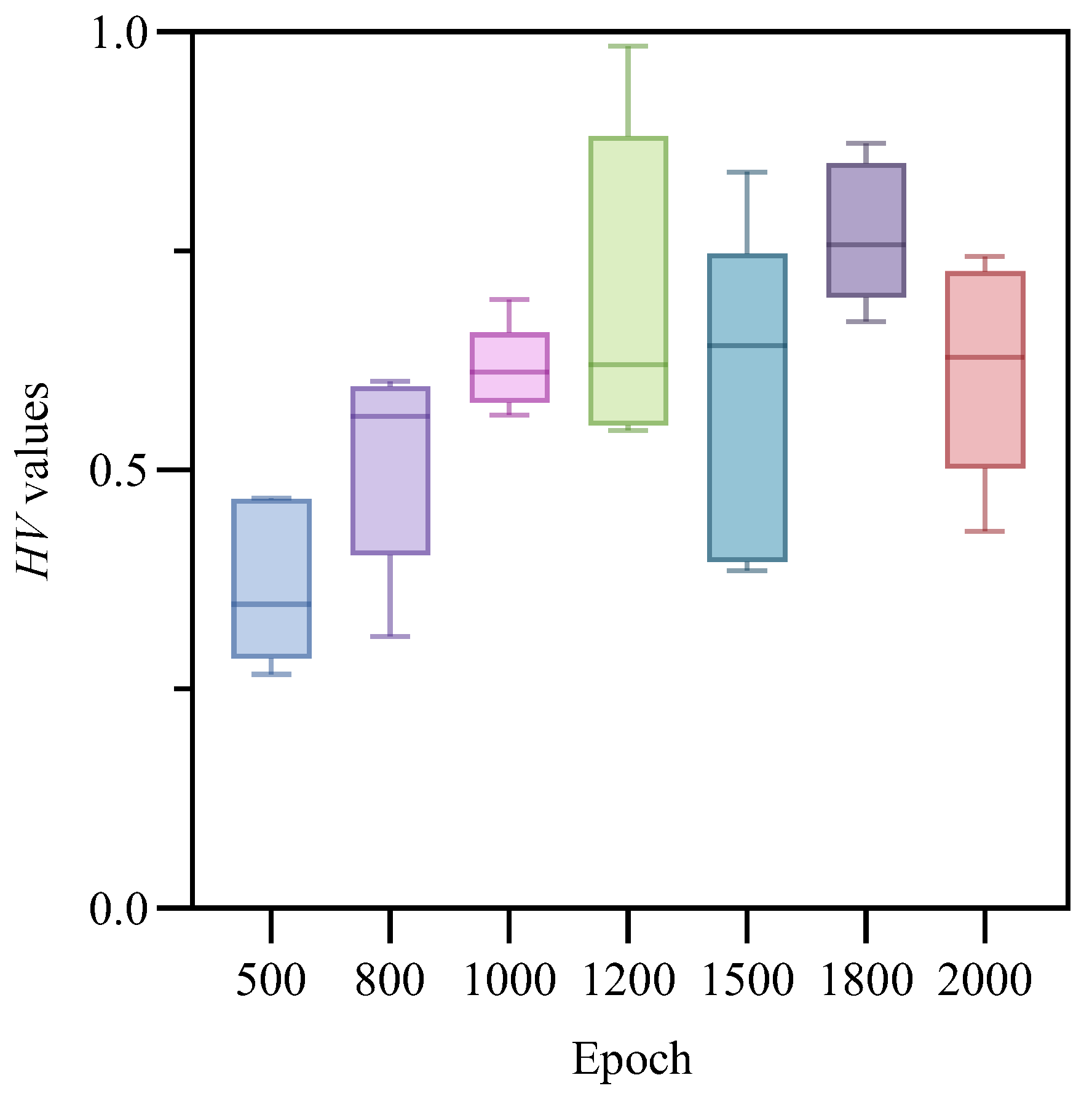
Figure 7. box plots of
HV values under different training epochs; different colors represent different numbers of training epochs. As shown in
Figure 7, across 10 runs of the algorithm, the model trained with 1800 epochs achieved an average
HV value of 0.767600375, which was higher than the other six settings (0.370214, 0.510288, 0.616378, 0.696846, 0.585371, and 0.617534, respectively). Therefore, the model trained for 1800 epochs overall produced the best results and demonstrated greater stability across multiple runs.
In addition, the hyperparameters of the two agents were tuned, and the optimal values were determined by monitoring the cumulative reward in each training epoch.
Table 8 and
Table 9 summarize the optimal parameter settings obtained from the experiments, while
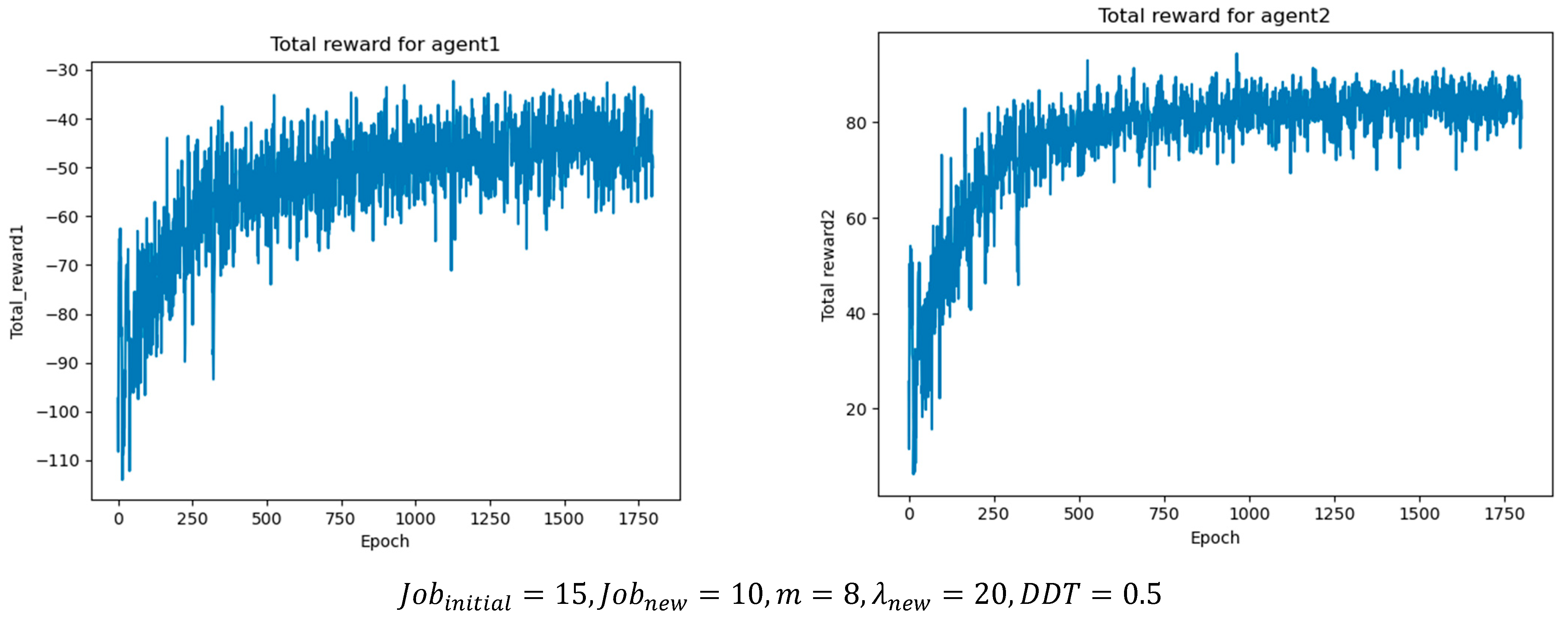
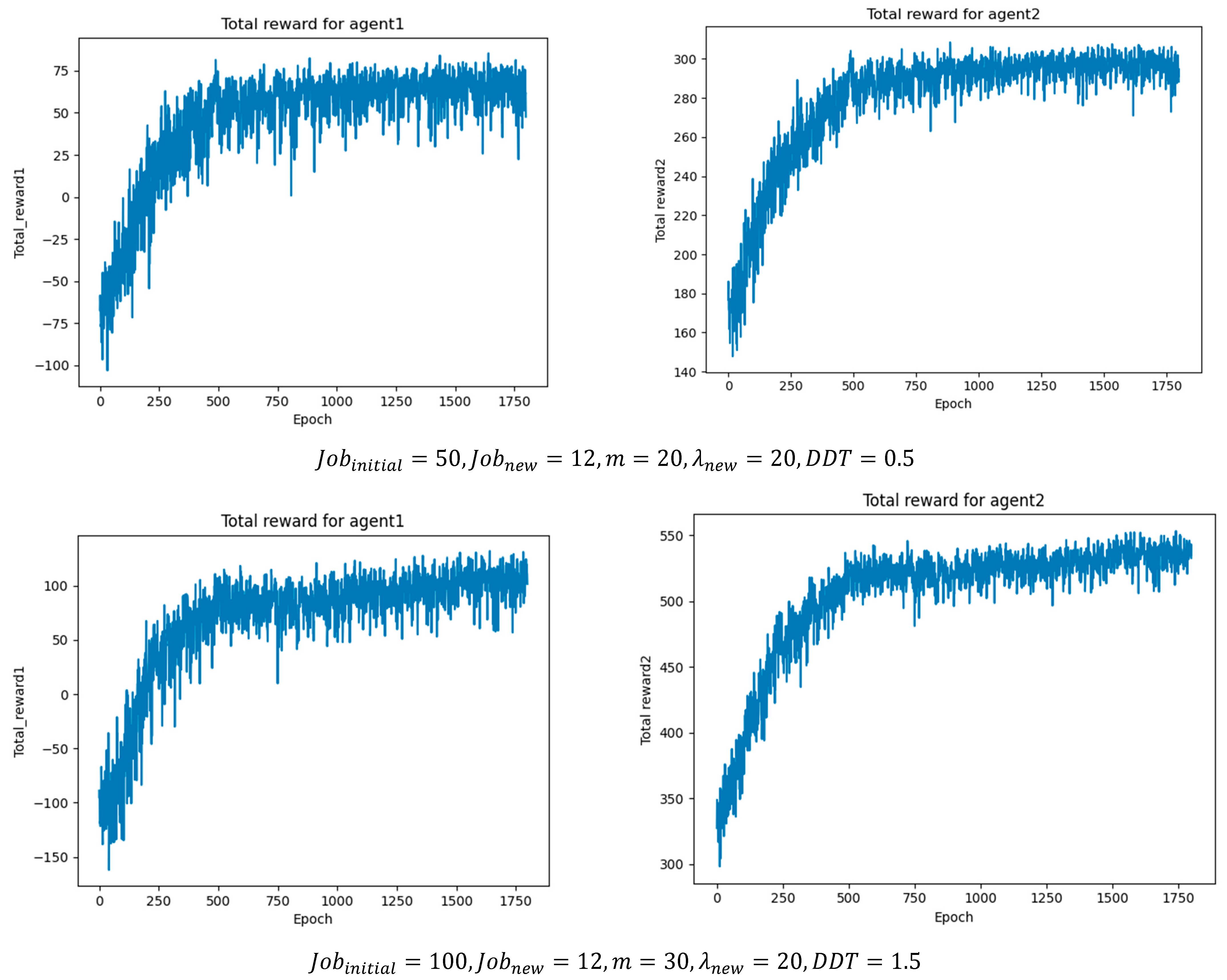
Figure 8 illustrates the cumulative reward results per epoch under different job batch sizes, where agent1 represents the job agent and agent2 represents the machine agent. As the batch size increases, the number of scheduling operations and optimal actions also rises, leading to higher cumulative rewards. This demonstrates that the proposed method can achieve stable convergence under different operating conditions.
5.4. Experimental Results
5.4.1. Comparison of Results
To evaluate the effectiveness and stability of the proposed multi-agent reinforcement learning framework in solving the MODFJSP described in this study, commonly used DRL baselines in the FJSP domain (PPO, DQN, DDQN) are selected for comparison [
12,
25,
26].
Table 10 lists several typical combinations of cooperative agents. In addition, classical scheduling rules applicable to the context of this study, as shown in
Table 11, are introduced as benchmarks [
22]. A systematic evaluation of solution quality is then conducted based on three evaluation metrics, with particular emphasis on maximizing net profit and minimizing makespan.
In this study, each method is independently executed 10 runs on 24 instances, and the average IGD and HV values as well as the SC metric are calculated to comprehensively evaluate the advantages and disadvantages of the proposed method compared with other approaches. Moreover, the dominance relationships between the non-dominated solutions generated by our method and those of the comparison methods are analyzed. The evaluation results are presented in
Table 12,
Table 13 and
Table 14, with the best values highlighted in bold.
First, for fixed composite scheduling rules such as EDD–SPT-M and FIFO–EAM, the lack of adaptability to optimization objectives often leads to repeatedly generating similar solutions for the two objectives, thereby limiting their optimization potential. Although random selection of jobs and machines provides exploratory capability, the strong randomness in decision-making makes it difficult to form a stable learning process and achieve convergence. In addition, among the reinforcement learning combinations, our proposed DDQN–DDQN method performs slightly worse than DDQN–DQN in large-scale scenarios with higher DDT values and a larger number of jobs. Nevertheless, their HV and IGD values remain close, indicating only minor differences in the overall quality of the Pareto front. Finally, although PPO has shown advantages in some FJSP studies, in this work its instability and low sample efficiency are amplified by the variable action sets and complex state representations, resulting in inferior overall performance compared with other reinforcement learning methods.
5.4.2. Visual Comparison of Results
For a deeper comparison,
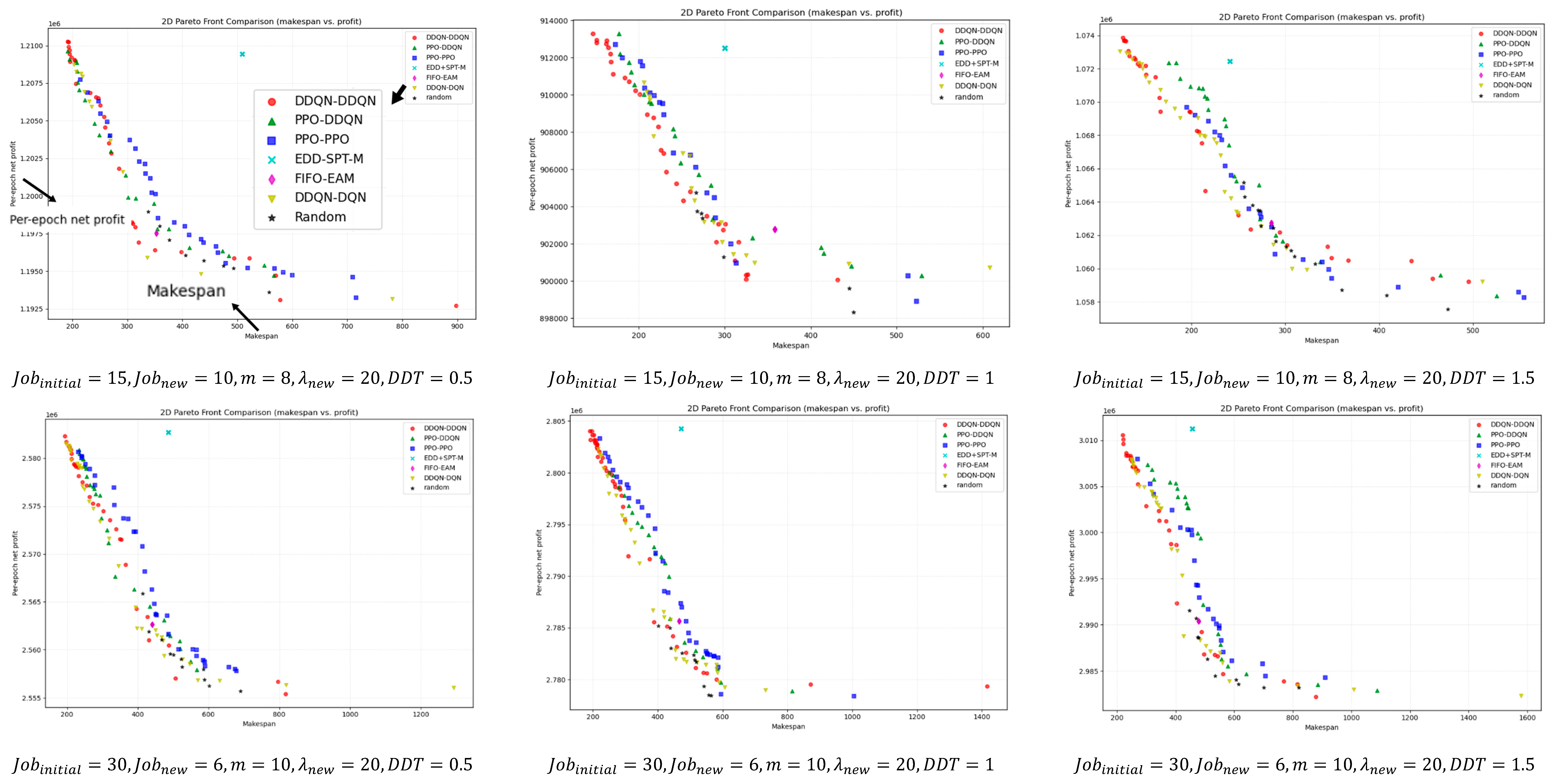
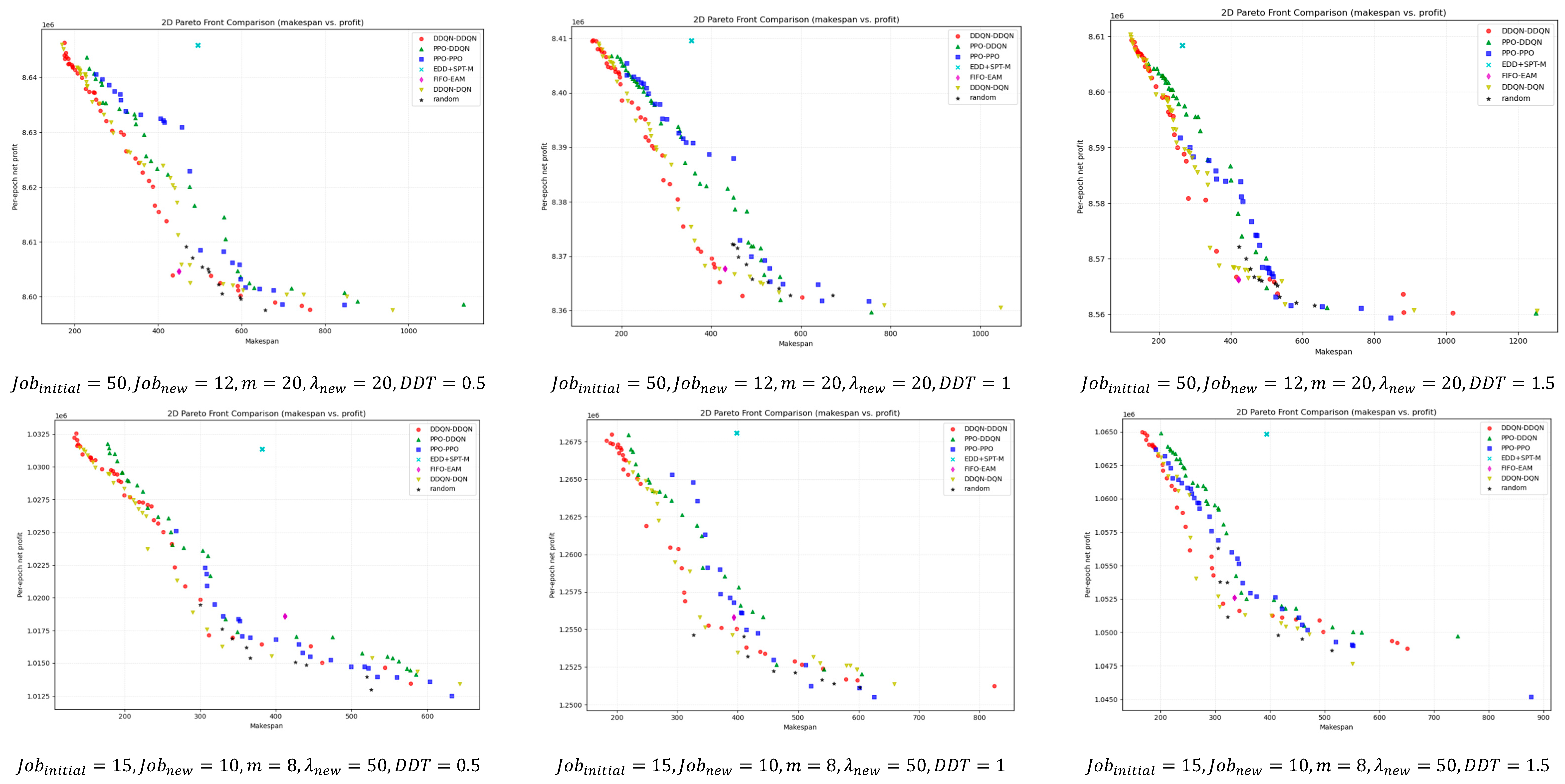
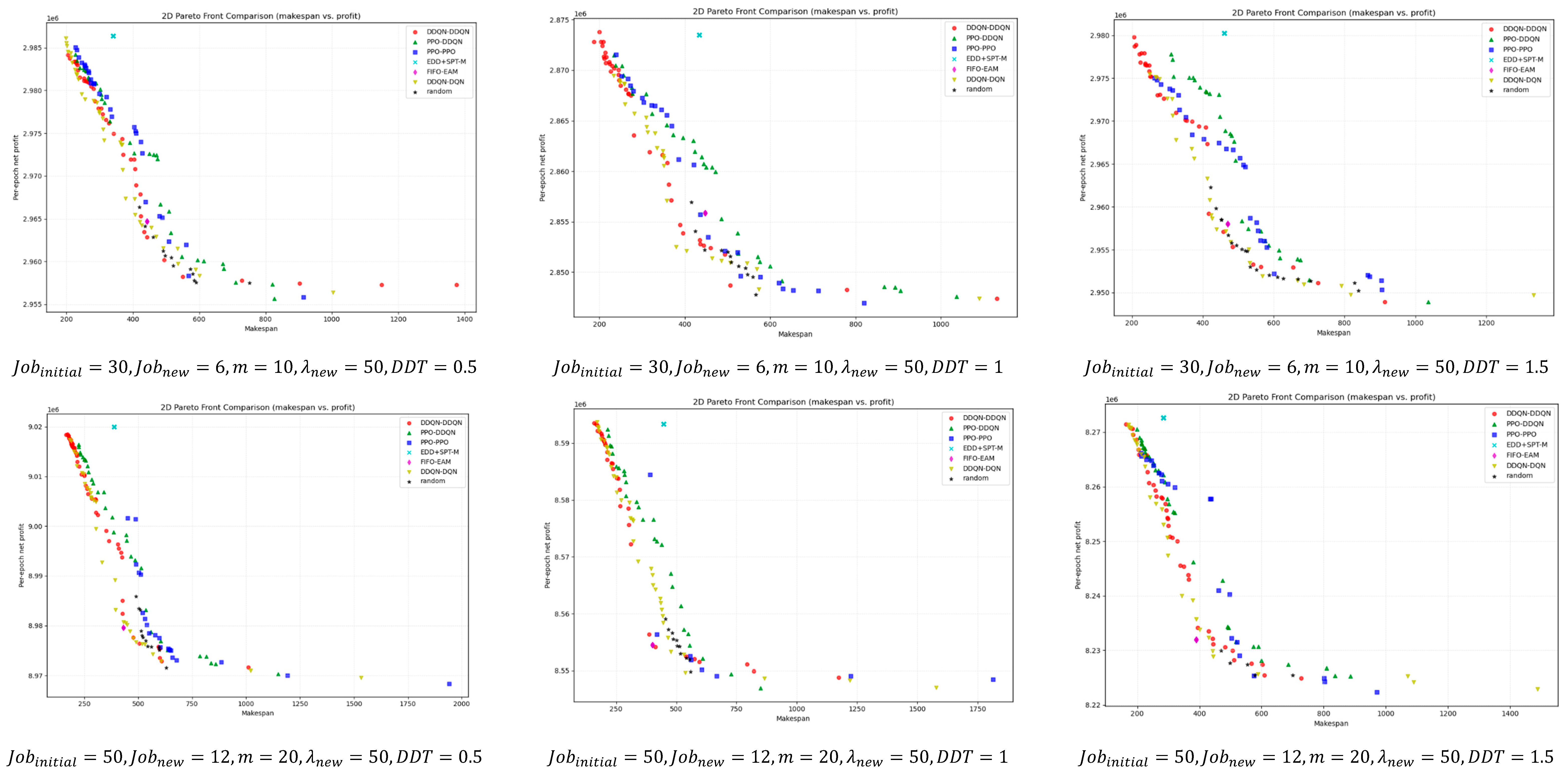
Figure 9 illustrates the bi-objective Pareto fronts obtained after non-dominated filtering for different instance scales. Overall, DDQN–DDQN is closer to the ideal point in most instances and maintains good front coverage. Even in the few cases where it does not outperform in terms of
HV,
IGD, or SC metrics, its pareto front remains close to that of the best-performing method, with only minor visual differences.
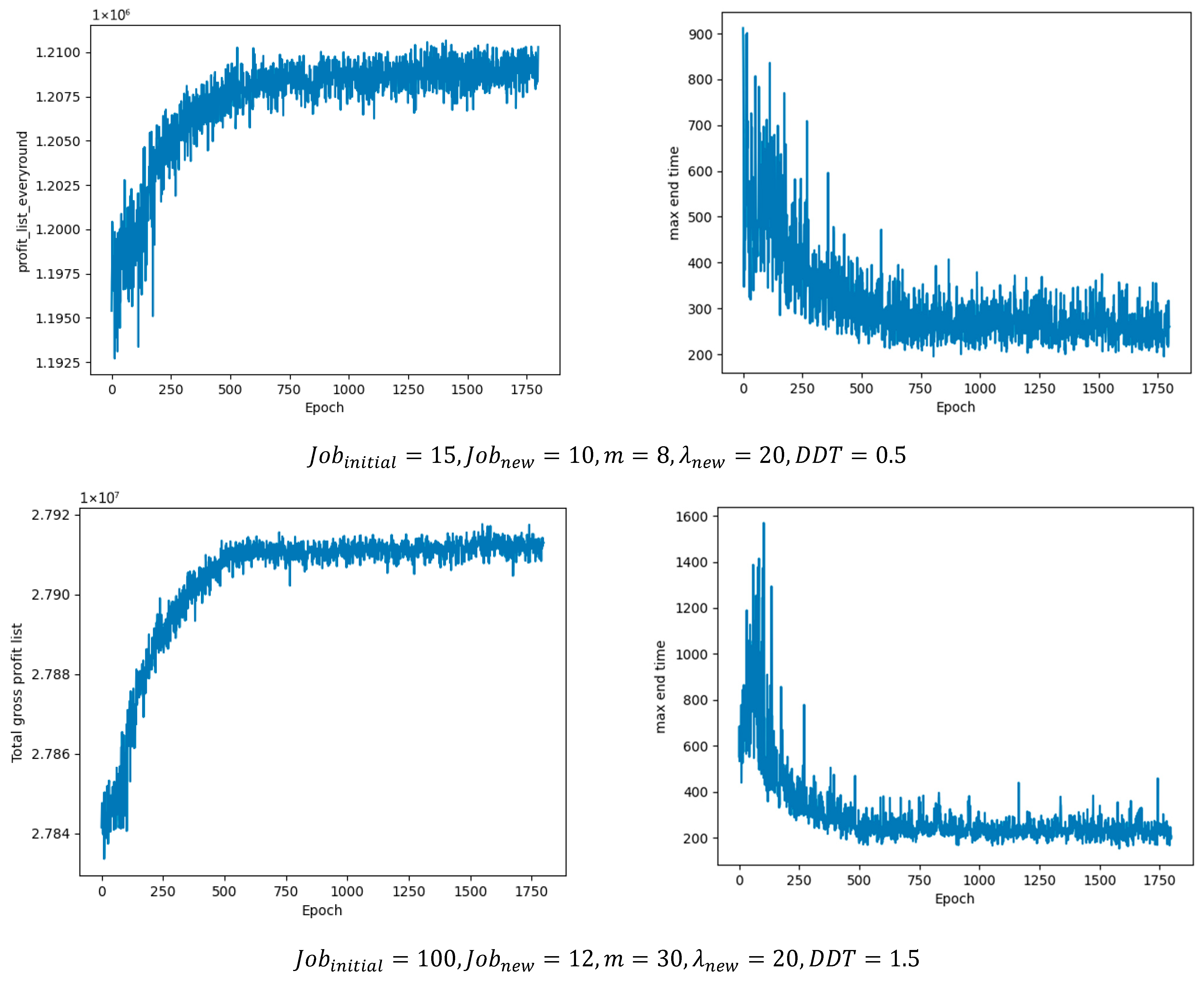
Unlike intelligent optimization algorithms that can generate multiple candidate solutions in parallel, DRL produces one scheduling solution per epoch. Guided by the reward functions and through continuous iterations, it can eventually approach the optimal solution. Specifically, the DRL agent interacts with the environment through actions, generating one scheduling solution in each training epoch; under the guidance of reward signals, it updates iteratively, gradually improving solution quality and finally converging to a (near-)optimal solution. As shown in
Figure 10, the proposed collaborative multi-agent method quickly explores high-reward solutions in the early training stage under reward-driven guidance, and subsequently stabilizes and converges to an approximately optimal solution.
5.5. Decision Support Module
Due to inherent conflicts between the two objectives, such as an excessive pursuit of low
Cmax potentially increasing the number of jobs processed simultaneously, thereby driving up electricity costs and reducing profits; conversely, maximizing profits may delay certain processes to off-peak electricity periods, consequently increasing
Cmax. To comprehensively evaluate the potential of the proposed model, the technique for order preference by similarity to ideal solution (TOPSIS) method is employed to identify optimal or near-optimal solutions among the non-inferior solutions [
41,
42].
Table 15 presents representative non-dominated solutions obtained by the algorithm.
Decision-makers can obtain the most satisfactory solution from non-inferior solutions using the TOPSIS method [
43]. First, establish weight vectors based on decision-makers’ preferences:
Cmax priority
W1 = [0.7, 0.3], profit priority
W2 = [0.3, 0.7].
Based on the Pareto solution design decision matrix
X in
Table 15Due to the differing dimensions of various objectives, it is challenging to evaluate performance metrics. By normalizing different values, a normalized decision matrix
Y is constructed.
Given a weight vector reflecting decision-maker preferences, the normalized matrix
Y is weighted row by row to obtain the weighted normalized matrix:
Since one objective should be as small as possible while the other should be as large as possible, the ideal solution and negative ideal solution can be defined as
Calculate the Euclidean distance between the ideal solution and the negative ideal solution:
Define the relative closeness coefficient using the TOPSIS method:
The larger
, the better the plan, which means it is based on the decision-maker’s preferences. Therefore,
Table 16 shows that the weight vector
W1 corresponds to “
Cmax priority,” and the optimal solution calculated based on this weight is S2; the weight vector
W2 corresponds to “profit priority,” and the optimal solution calculated based on this weight is
S3.
6. Conclusions
In this study, for the MODFJSP, we construct a “job selection–machine assignment” multi-agent collaborative framework that comprehensively considers factors such as dynamic job arrivals, fluctuating due dates, and high-profit urgent orders, with the dual objectives of maximizing net profit and minimizing makespan. In terms of method design, variable state representations, reward functions, and variable action spaces are customized for the two types of agents to enhance learning efficiency and stability. Systematic experiments are then conducted on 18 instances, comparing the proposed framework with PPO, DQN, and other deep reinforcement learning algorithms as well as classical scheduling rules. The results show that the proposed framework demonstrates a certain advantage in solution quality and robustness. Statistics indicate that, compared with other algorithms and scheduling rules, it can achieve a 0.368% increase in profit.
The profit function employed by this research does not account for labor, maintenance, inventory, or other financial factors, thus retaining a certain gap from real-world business metrics. Furthermore, the methodology has not yet been validated against traditional heuristic algorithms, and its effectiveness and advantages require further exploration.
Subsequent work will focus on integrating more practical profit functions and introducing more robust and efficient multi-agent reinforcement learning algorithms to optimize the overall trade-off between profitability and timeliness in dynamic and uncertain industrial environments. Additionally, flexible profit models may be considered, enabling users to adjust profit parameters according to actual needs, thereby enhancing the model’s applicability and practical value.
Author Contributions
Q.M.: Conceptualization, Writing—Original Draft, Formal analysis, Data curation, Visualization, Software, Funding acquisition. Y.L.: Methodology, Conceptualization, Formal analysis, Writing—Review & Editing, Funding acquisition, Supervision. H.C.: Supervision, Writing—Review & Editing. All authors have read and agreed to the published version of the manuscript.
Funding
The research reported in this paper is financially supported by the Graduate Research Fund of Guizhou Province (Grant No. 2024YJSKYJJ165), and the Guizhou Provincial Basic Research Program (Natural Science) (Grant No. Qian Ke He Ji Chu-ZK [2024] General 439).
Data Availability Statement
Conflicts of Interest
The authors declare that they have no known competing financial interests or personal relationships that could have appeared to influence the work reported in this paper.
Abbreviations
The following abbreviations are used in this manuscript:
| Acronym | Full name | Explanation |
| RL | Reinforcement learning | A machine learning paradigm where an agent learns to make sequential decisions by interacting with an environment, receiving rewards or penalties, and optimizing its policy to maximize long-term cumulative reward. |
| DRL | Deep reinforcement learning | A method that combines deep learning with reinforcement learning to solve sequential decision-making problems in high-dimensional state and action spaces. |
| MDP | Markov decision process | A mathematical framework to formalize reinforcement learning environments, defined by states, actions, rewards, and transition probabilities. |
| TOU | Time of use | An electricity pricing scheme where the unit price of electricity varies depending on the time of day, encouraging users to shift consumption to off-peak periods. |
| PPO | Proximal policy optimization | An improved policy gradient algorithm that constrains policy updates to ensure training stability and higher sample efficiency. |
| DQN | Deep Q learning | A reinforcement learning algorithm that combines deep neural networks with Q-learning to approximate the action-value function. |
| DDQN | Double deep Q-network | An extension of DQN that uses two networks to reduce overestimation bias in Q-value estimation, improving performance. |
| MODFJSP | Multi-objective dynamic flexible job shop scheduling | A scheduling problem that considers both dynamic environments and multiple optimization objectives. |
| SC | Set coverage | A metric used to evaluate the coverage of a solution set across a set of test instances. |
| IGD | Inverted generational distance | A performance indicator that measures how close the obtained solutions are to the true Pareto front. |
| HV | Hypervolume | A metric that evaluates the volume covered by a solution set in the objective space, reflecting both convergence and diversity. |
| JSP | Job shop scheduling problem | A classical scheduling problem where jobs must be processed on machines, typically aiming to minimize makespan or delays. |
| FJSP | Flexible job shop scheduling problem | An extension of JSP that allows operations to be assigned to one of several alternative machines. |
| DFJSP | Dynamic flexible job shop scheduling problem | A further extension of FJSP that accounts for dynamic job arrivals and environmental uncertainties. |
| Cmax | Max end time (Makespan). | The maximum completion time of all jobs, often used as a key optimization objective in scheduling. |
| TOPSIS | Technique for order preference by similarity to ideal solution | A multi-criteria decision-making method that ranks alternatives based on their relative closeness to an ideal and anti-ideal solution. |
References
- Geng, K.; Liu, L.; Wu, S. A Reinforcement Learning Based Memetic Algorithm for Energy-Efficient Distributed Two-Stage Flexible Job Shop Scheduling Problem. Sci. Rep. 2024, 14, 30816. [Google Scholar] [CrossRef]
- Peng, W.; Yu, D.; Xie, F. Multi-Mode Resource-Constrained Project Scheduling Problem with Multiple Shifts and Dynamic Energy Prices. Int. J. Prod. Res. 2025, 63, 2483–2506. [Google Scholar] [CrossRef]
- Luo, C.; Gong, W.; Lu, C. Knowledge-Driven Two-Stage Memetic Algorithm for Energy-Efficient Flexible Job Shop Scheduling with Machine Breakdowns. Expert Syst. Appl. 2024, 235, 121149. [Google Scholar] [CrossRef]
- Yao, Y.; Li, X.; Gao, L. A DQN-Based Memetic Algorithm for Energy-Efficient Job Shop Scheduling Problem with Integrated Limited AGVs. Swarm Evol. Comput. 2024, 87, 101544. [Google Scholar] [CrossRef]
- Destouet, C.; Tlahig, H.; Bettayeb, B.; Mazari, B. Flexible Job Shop Scheduling Problem under Industry 5.0: A Survey on Human Reintegration, Environmental Consideration and Resilience Improvement. J. Manuf. Syst. 2023, 67, 155–173. [Google Scholar] [CrossRef]
- Zhang, Q.; Shao, W.; Shao, Z.; Pi, D.; Gao, J. Deep Reinforcement Learning Driven Trajectory-Based Meta-Heuristic for Distributed Heterogeneous Flexible Job Shop Scheduling Problem. Swarm Evol. Comput. 2024, 91, 101753. [Google Scholar] [CrossRef]
- Yu, W.; Zhang, L.; Ge, N. An Adaptive Multiobjective Evolutionary Algorithm for Dynamic Multiobjective Flexible Scheduling Problem. Int. J. Intell. Syst. 2022, 37, 12335–12366. [Google Scholar] [CrossRef]
- Lv, L.; Fan, J.; Zhang, C.; Shen, W. A Multi-Agent Reinforcement Learning Based Scheduling Strategy for Flexible Job Shops under Machine Breakdowns. Robot. Comput. Integr. Manuf. 2025, 93, 102923. [Google Scholar] [CrossRef]
- Zhao, F.; Wang, W.; Zhu, N.; Xu, T. An Inverse Reinforcement Learning Algorithm with Population Evolution Mechanism for the Multi-Objective Flexible Job-Shop Scheduling Problem under Time-of-Use Electricity Tariffs. Appl. Soft Comput. 2025, 170, 112764. [Google Scholar] [CrossRef]
- Ahmadi, E.; Zandieh, M.; Farrokh, M.; Emami, S.M. A Multi Objective Optimization Approach for Flexible Job Shop Scheduling Problem under Random Machine Breakdown by Evolutionary Algorithms. Comput. Oper. Res. 2016, 73, 56–66. [Google Scholar] [CrossRef]
- Wang, H.; Cheng, J.; Liu, C.; Zhang, Y.; Hu, S.; Chen, L. Multi-Objective Reinforcement Learning Framework for Dynamic Flexible Job Shop Scheduling Problem with Uncertain Events. Appl. Soft Comput. 2022, 131, 109717. [Google Scholar] [CrossRef]
- Lei, K.; Guo, P.; Zhao, W.; Wang, Y.; Qian, L.; Meng, X.; Tang, L. A Multi-Action Deep Reinforcement Learning Framework for Flexible Job-Shop Scheduling Problem. Expert Syst. Appl. 2022, 205, 117796. [Google Scholar] [CrossRef]
- Lv, Z.; Zhao, Y.; Kang, H.; Gao, Z.; Qin, Y. An Improved Harris Hawk Optimization Algorithm for Flexible Job Shop Scheduling Problem. Comput. Mater. Contin. 2024, 78, 2337–2360. [Google Scholar] [CrossRef]
- Wang, Z.; He, M.; Wu, J.; Chen, H.; Cao, Y. An Improved MOEA/D for Low-Carbon Many-Objective Flexible Job Shop Scheduling Problem. Comput. Ind. Eng. 2024, 188, 109926. [Google Scholar] [CrossRef]
- Zhang, X.; Zhu, G.-Y. A Literature Review of Reinforcement Learning Methods Applied to Job-Shop Scheduling Problems. Comput. Oper. Res. 2025, 175, 106929. [Google Scholar] [CrossRef]
- Catanzaro, D.; Pesenti, R.; Ronco, R. Job Scheduling under Time-of-Use Energy Tariffs for Sustainable Manufacturing: A Survey. Eur. J. Oper. Res. 2023, 308, 1091–1109. [Google Scholar] [CrossRef]
- Shen, L.; Dauzère-Pérès, S.; Maecker, S. Energy Cost Efficient Scheduling in Flexible Job-Shop Manufacturing Systems. Eur. J. Oper. Res. 2023, 310, 992–1016. [Google Scholar] [CrossRef]
- Park, M.-J.; Ham, A. Energy-Aware Flexible Job Shop Scheduling under Time-of-Use Pricing. Int. J. Prod. Econ. 2022, 248, 108507. [Google Scholar] [CrossRef]
- Zouadi, T.; Chargui, K.; Zhani, N.; Charles, V.; Sreedharan, V.R. A Novel Robust Decomposition Algorithm for a Profit-Oriented Production Routing Problem with Backordering, Uncertain Prices, and Service Level Constraints. Ann. Oper. Res. 2024, 341, 1361–1362. [Google Scholar] [CrossRef]
- Yuan, E.; Wang, L.; Song, S.; Cheng, S.; Fan, W. Dynamic Scheduling for Multi-Objective Flexible Job Shop via Deep Reinforcement Learning. Appl. Soft Comput. 2025, 171, 112787. [Google Scholar] [CrossRef]
- Zhang, C.; Juraschek, M.; Herrmann, C. Deep Reinforcement Learning-Based Dynamic Scheduling for Resilient and Sustainable Manufacturing: A Systematic Review. J. Manuf. Syst. 2024, 77, 962–989. [Google Scholar] [CrossRef]
- Luo, S. Dynamic Scheduling for Flexible Job Shop with New Job Insertions by Deep Reinforcement Learning. Appl. Soft Comput. 2020, 91, 106208. [Google Scholar] [CrossRef]
- Lu, S.; Wang, Y.; Kong, M.; Wang, W.; Tan, W.; Song, Y. A Double Deep Q-Network Framework for a Flexible Job Shop Scheduling Problem with Dynamic Job Arrivals and Urgent Job Insertions. Eng. Appl. Artif. Intell. 2024, 133, 108487. [Google Scholar] [CrossRef]
- Wang, H.; Lin, W.; Peng, T.; Xiao, Q.; Tang, R. Multi-Agent Deep Reinforcement Learning-Based Approach for Dynamic Flexible Assembly Job Shop Scheduling with Uncertain Processing and Transport Times. Expert Syst. Appl. 2025, 270, 126441. [Google Scholar] [CrossRef]
- Liu, R.; Piplani, R.; Toro, C. Deep Reinforcement Learning for Dynamic Scheduling of a Flexible Job Shop. Int. J. Prod. Res. 2022, 60, 4049–4069. [Google Scholar] [CrossRef]
- Yan, Y.; Yi, W.; Pei, Z.; Chen, Y. Multi-Agent Reinforcement Learning for Distributed Flexible Job Shop Scheduling with Random Job Arrival. IEEE Access 2025, 13, 80941–80957. [Google Scholar] [CrossRef]
- Popper, J.; Ruskowski, M. Using multi-agent deep reinforcement learning for flexible job shop scheduling problems. Procedia CIRP 2022, 112, 63–67. [Google Scholar] [CrossRef]
- Yu, K.; Jin, K.; Deng, X. Review of Deep Reinforcement Learning. In Proceedings of the 2022 IEEE 5th Advanced Information Management, Communicates, Electronic and Automation Control Conference (IMCEC), Chongqing, China, 16 December 2022; IEEE: New York, NY, USA, 2022; pp. 41–48. [Google Scholar]
- Kaloev, M.; Krastev, G. Experiments Focused on Exploration in Deep Reinforcement Learning. In Proceedings of the 2021 5th International Symposium on Multidisciplinary Studies and Innovative Technologies (ISMSIT), Ankara, Turkey, 21 October 2021; IEEE: New York, NY, USA, 2021; pp. 351–355. [Google Scholar]
- Wan, L.; Cui, X.; Zhao, H.; Li, C.; Wang, Z. An Effective Deep Actor-Critic Reinforcement Learning Method for Solving the Flexible Job Shop Scheduling Problem. Neural Comput. Appl. 2024, 36, 11877–11899. [Google Scholar] [CrossRef]
- Yue, L.; Peng, K.; Ding, L.; Mumtaz, J.; Lin, L.; Zou, T. Two-Stage Double Deep Q-Network Algorithm Considering External Non-Dominant Set for Multi-Objective Dynamic Flexible Job Shop Scheduling Problems. Swarm Evol. Comput. 2024, 90, 101660. [Google Scholar] [CrossRef]
- Yuan, M.; Huang, H.; Li, Z.; Zhang, C.; Pei, F.; Gu, W. A Multi-Agent Double Deep-Q-Network Based on State Machine and Event Stream for Flexible Job Shop Scheduling Problem. Adv. Eng. Inform. 2023, 58, 102230. [Google Scholar] [CrossRef]
- Luo, S.; Zhang, L.; Fan, Y. Dynamic Multi-Objective Scheduling for Flexible Job Shop by Deep Reinforcement Learning. Comput. Ind. Eng. 2021, 159, 107489. [Google Scholar] [CrossRef]
- Chen, W.; Wang, J.; Yu, G. Energy-Efficient Scheduling for a Hybrid Flow Shop Problem While Considering Multi-Renewable Energy. Int. J. Prod. Res. 2024, 62, 8352–8372. [Google Scholar] [CrossRef]
- Zitzler, E.; Thiele, L. Multiobjective Evolutionary Algorithms: A Comparative Case Study and the Strength Pareto Approach. IEEE Trans. Evol. Comput. 1999, 3, 257–271. [Google Scholar] [CrossRef]
- Coello, C.A.C.; Cortés, N.C. Solving Multiobjective Optimization Problems Using an Artificial Immune System. Genet. Program. Evolvable Mach. 2005, 6, 163–190. [Google Scholar] [CrossRef]
- Wang, J.; Wu, C.; Peng, Y. Multi-Objective Scheduling for an Energy-Efficient Flexible Job Shop Problem with Peak Power Constraint. Appl. Soft Comput. 2024, 167, 112330. [Google Scholar] [CrossRef]
- Wei, L.; He, J.; Guo, Z.; Hu, Z. A Multi-Objective Migrating Birds Optimization Algorithm Based on Game Theory for Dynamic Flexible Job Shop Scheduling Problem. Expert Syst. Appl. 2023, 227, 120268. [Google Scholar] [CrossRef]
- Wu, J.; Liu, Y. A Modified Multi-Agent Proximal Policy O ptimization Algorithm for Multi-Objective Dynamic Partial-Re-Entrant Hybrid Flow Shop Scheduling Problem. Eng. Appl. Artif. Intell. 2025, 140, 109688. [Google Scholar] [CrossRef]
- Serrano-Ruiz, J.C.; Mula, J.; Poler, R. Job Shop Smart Manufacturing Scheduling by Deep Reinforcement Learning. J. Ind. Inf. Integr. 2024, 38, 100582. [Google Scholar] [CrossRef]
- Wang, Y.-M.; Elhag, T.M.S. Fuzzy TOPSIS Method Based on Alpha Level Sets with an Application to Bridge Risk Assessment. Expert Syst. Appl. 2006, 31, 309–319. [Google Scholar] [CrossRef]
- Roy, A.; Wallenius, J. Nonlinear and Unconstrained Multiple-Objective Optimization: Algorithm, Computation, and Application. Nav. Res. Logist. 1991, 38, 623–635. [Google Scholar] [CrossRef]
- Dai, M.; Tang, D.; Giret, A.; Salido, M.A. Multi-Objective Optimization for Energy-Efficient Flexible Job Shop Scheduling Problem with Transportation Constraints. Robot. Comput. Integr. Manuf. 2019, 59, 143–157. [Google Scholar] [CrossRef]
Figure 1.
The framework model of the MODFJSP considered in this study.
Figure 1.
The framework model of the MODFJSP considered in this study.
Figure 2.
RL framework under the MDP.
Figure 2.
RL framework under the MDP.
Figure 3.
Multi-agent collaborative framework of “job selection–machine assignment”.
Figure 3.
Multi-agent collaborative framework of “job selection–machine assignment”.
Figure 4.
Structure of the job agent.
Figure 4.
Structure of the job agent.
Figure 5.
Structure of the machine agent.
Figure 5.
Structure of the machine agent.
Figure 6.
Decision-making sequence of the proposed multi-agent framework for MODFJSP.
Figure 6.
Decision-making sequence of the proposed multi-agent framework for MODFJSP.
Figure 7.
Boxplot of HV values across different epochs.
Figure 7.
Boxplot of HV values across different epochs.
Figure 8.
Cumulative rewards per epoch under different operating conditions.
Figure 8.
Cumulative rewards per epoch under different operating conditions.
Figure 9.
Bi-objective Pareto fronts across instance scales after non-dominated filtering.
Figure 9.
Bi-objective Pareto fronts across instance scales after non-dominated filtering.
Figure 10.
Per-epoch convergence of each objective on different problem scales.
Figure 10.
Per-epoch convergence of each objective on different problem scales.
Table 1.
Studies on DRL-based flexible job shop scheduling problems.
Table 1.
Studies on DRL-based flexible job shop scheduling problems.
| Work | RL Algorithm | Agent | Problem | Dynamic Events | Objectives |
|---|
| [22] | DQN | Single | DFJSP | New job insertions | Tardiness |
| [23] | DDQN | Single | MODFJSP | New job insertions and urgent job insertions | Cmax, Tardiness |
| [12] | PPO | Single | FJSP | None | Cmax |
| [25] | DDQN | Multiple | DFJSP | New job insertions | Total tardiness |
| [26] | DQN | Multiple | DFJSP | New job insertions | Total tardiness |
| [27] | PPO | Multiple | FJSP with AGVs | None | Makespan; Average lateness; Max lateness |
| Our work | DDQN | Multiple | MODFJSP | New job insertions, high-profit urgent job insertions, and due day changes | Cmax, Total net Profit |
Table 2.
Notations for the mathematical model.
Table 2.
Notations for the mathematical model.
| Parameters | Description |
|---|
| Set of n jobs, with = {1, 2, …, n}. |
| Set of machines, with M = {1, 2, …, m}. |
| Set of operations of job i, with = {1, …, ni}. |
| Set of all time points within the entire scheduling time horizon, with T = {1,2, 3, …, Cmax}. |
| Set of unfinished jobs at decision point st. |
| Set of urgent jobs. |
| Processing time of operation Oi,j on machine k, , , . |
| Number of newly arrived jobs. |
| The set of available machines for operation, , . |
| Selling price of job i, i.e., the price offered by the customer, . |
| TOU electricity price (yuan/kWh) at time t, . |
| Tardiness of job i, . |
| Energy processing consumption of machine k (kW), . |
| Idle power consumption of machine k (kW), . |
| Total power consumption of the shop at time t (kW): , including both processing and idle power consumption, , , . |
| Urgency level of urgent jobs, , . |
| Net profit of job i, . |
| Index of the operation of job i completed at scheduling point st, . |
| Tardiness penalty of job i, . |
| Ci | Completion time of job i. |
| Ci,j | Completion time of operation Oi,j. |
| Variables | Description |
| Time-related task and resource allocation variables: at time t, operation Oi,j of job j being processed on machine k is 1. |
| Equal to 1 if and only if machine k is in the ON state. |
Table 3.
Explanation of variables covered in
Section 4.
Table 3.
Explanation of variables covered in
Section 4.
| Parameters | Description |
|---|
| At decision point st, the set of job states. = {} |
| The state corresponding to job i at the decision point, where |
| At decision point st, the set of available machine statuses for the next machining operation of the selected job. = {} |
| The state corresponding to machine k, |
| Index of completed machining operations for job i, where |
| Job agent reward |
| Machine agent reward |
| Job i delay time |
| Action space of the job agent |
| Action space of machine agent |
| At decision point st, the action taken by the job agent is to select the job state with the highest Q-value. |
| At decision point st, the job index corresponding to the job state selected by |
| At decision point st, the action taken by the machine agent is the selection of the machine state with the highest Q-value. |
| At decision point st, the machine index corresponding to |
| DDQN soft update parameters. |
Table 4.
Descriptions of the state input variables of the job agent.
Table 4.
Descriptions of the state input variables of the job agent.
| Features | Description |
|---|
| Job index, where denotes the set of unfinished jobs. |
| Ratio of the remaining operations to the total operations of the job. |
| Estimated remaining processing time intensity based on the average operation processing time, normalized. |
| Urgency level of the job, set to 0 if it is not an urgent job. |
| Urgent job indicator: 1 if job i belongs to the urgent job set, and 0 otherwise. |
| Normalized profit of job i. |
Table 5.
Descriptions of the available machine state variables.
Table 5.
Descriptions of the available machine state variables.
| Features | Description |
|---|
| k | Machine index, |
| Power of the machine when processing the operation, normalized by the maximum power |
| Processing time of machine k for operation , normalized by the maximum processing time among its available machines |
| Estimated electricity cost incurred by processing on machine k. |
| Available start time of machine k for processing the pending operation of job , normalized by the maximum available time of all machines. |
| Estimated profit generated by processing on machine k, normalized by the maximum profit among all candidates. |
Table 6.
Parameter settings of numerical simulation instances.
Table 6.
Parameter settings of numerical simulation instances.
| Parameters | Value |
|---|
| Set of the number of initial jobs | {15, 30, 50, 100} |
| Set of the number of new inserted jobs | {10, 6, 12} |
| Processing time per operation | U {1, 50} |
| Set of the number of total machines m | {8, 10, 20, 30} |
| Processing energy consumption | U {12, 17}KW |
| Idle power | 30% × |
| Due date tightness DDT | {0.5, 1, 1.5} |
| λnew | {20, 50} |
| Number of available machines of each operation | U {1, m − 1} |
| Number of operations belonging to a job | U {1, 5} |
| Number of urgent jobs | 20% of total jobs |
| Non-urgent profit | |
| Profit adjustment for urgent jobs | |
| Tardiness penalty for job i | |
Table 7.
TOU price.
| | TOU Power
| Period of Time |
|---|
Electricity purchase
price (yuan/kWh) | Peak: 1.241 | 9:00~12:00; 17:00~22:00 |
| Flat: 0.779 | 8:00~9:00; 12:00~17:00; 22:00~23:00 |
| Valley: 0.488 | 0:00~8:00; 23:00~24:00 |
Table 8.
Job agent parameter settings.
Table 8.
Job agent parameter settings.
| Hyperparameters | Value |
|---|
| Number of training epochs L | 1800 |
| Learning rate | 1 × 10⁻³ |
| Discount factor γ | 0.99 |
| ε-greedy exploration rate | 0.1 |
| Minimum ε-value | 0.05 |
| Batch size 1 | 64 |
| Buffer capacity | 10,000 |
| Soft update coefficient | 0.01 |
| Optimizer | Adam |
| Weight parameters in the reward function: | 6, 4 |
Table 9.
Machine agent parameter settings.
Table 9.
Machine agent parameter settings.
| Hyperparameters | Value |
|---|
| Number of training epochs L | 1800 |
| Learning rate | 1 × 10⁻³ |
| Discount factor γ | 0.99 |
| ε-greedy exploration rate | 0.1 |
| Minimum ε-value | 0.05 |
| Batch size 2 | 64 |
| Buffer capacity | 10,000 |
| Soft update coefficient | 0.01 |
| Optimizer | Adam |
| Weight parameters in the reward function: | 5, 4 |
Table 10.
Description of compared algorithms.
Table 10.
Description of compared algorithms.
| Algorithms | Description |
|---|
| DDQN-DDQN | Our method: Job agent with DDQN; Machine agent with DDQN |
| DDQN-DQN | Job agent with DDQN; Machine agent with DQN |
| PPO-DDQN | Job agent with PPO; Machine agent with DDQN |
| PPO-PPO | Job agent with PPO; Machine agent with PPO |
Table 11.
Description of scheduling rules.
Table 11.
Description of scheduling rules.
| Rules | Priority Description |
|---|
| EDD-SPT-M | Job selection: EDD prioritizes the job with the earliest due date; Machine selection: SPT-M prioritizes the machine with the shortest processing time. |
| FIFO-EAM | Job selection: FIFO prioritizes the earliest arriving job; Machine selection: EAM prioritizes the earliest available machine. |
| Random | Randomly select both job and machine. |
Table 12.
IGD values for solutions obtained by DDQN–DDQN, DDQN–DQN,PPO-DDQN, PPO-PPO and classical scheduling rules.
Table 12.
IGD values for solutions obtained by DDQN–DDQN, DDQN–DQN,PPO-DDQN, PPO-PPO and classical scheduling rules.
| DDT | | DDQN-DDQN | PPO-DDQN | PPO-PPO | DDQN-DQN | FIFO-EAM | EDD-SPT-M | Random |
|---|
| 20 | 0.5 | (15,10,8) | 0.054859 | 0.057435 | 0.173360 | 0.061103 | 0.380170 | 0.490278 | 0.289240 |
| (30,6,10) | 0.042265 | 0.051395 | 0.104919 | 0.0445135 | 0.420481 | 0.483181 | 0.300935 |
| (50,12,20) | 0.022450 | 0.039487 | 0.149944 | 0.027592 | 0.494244 | 0.411686 | 0.405403 |
| (100,12,30) | 0.000510 | 0.010893 | 0.093641 | 0.002407 | 0.338582 | 0.537263 | 0.437711 |
| 1 | (15,10,8) | 0.053759 | 0.074556 | 0.084140 | 0.056995 | 0.352341 | 0.439906 | 0.154800 |
| (30,6,10) | 0.044555 | 0.064114 | 0.084884 | 0.052853 | 0.360538 | 0.542772 | 0.305371 |
| (50,12,20) | 0.029263 | 0.048181 | 0.107453 | 0.032112 | 0.436225 | 0.451014 | 0.361074 |
| (100,12,30) | 0.097993 | 0.071701 | 0.019414 | 0.105504 | 0.04047 | 0.405968 | 0.110002 |
| 1.5 | (15,10,8) | 0.060887 | 0.089392 | 0.160640 | 0.050309 | 0.332754 | 0.447768 | 0.185778 |
| (30,6,10) | 0.042315 | 0.070105 | 0.117966 | 0.044867 | 0.408433 | 0.46043 | 0.323373 |
| (50,12,20) | 0.054425 | 0.061335 | 0.071502 | 0.044325 | 0.044744 | 0.790365 | 0.399020 |
| (100,12,30) | 0.049678 | 0.040152 | 0.106691 | 0.015308 | 0.090093 | 0.104488 | 0.092739 |
| 50 | 0.5 | (15,10,8) | 0.047233 | 0.063687 | 0.274370 | 0.05187 | 0.417043 | 0.464195 | 0.301849 |
| (30,6,10) | 0.048418 | 0.052739 | 0.061828 | 0.042306 | 0.355806 | 0.595167 | 0.268373 |
| (50,12,20) | 0.034162 | 0.061210 | 0.080823 | 0.050394 | 0.044621 | 0.740737 | 0.264720 |
| (100,12,30) | 0.037861 | 0.04037 | 0.07939 | 0.040909 | 0.044794 | 0.400768 | 0.441831 |
| 1 | (15,10,8) | 0.045325 | 0.064684 | 0.161846 | 0.059643 | 0.365292 | 0.492496 | 0.331768 |
| (30,6,10) | 0.394420 | 0.060557 | 0.076853 | 0.048337 | 0.387177 | 0.433037 | 0.309464 |
| (50,12,20) | 0.062509 | 0.076393 | 0.086067 | 0.054579 | 0.333961 | 0.782902 | 0.372529 |
| (100,12,30) | 0.070671 | 0.039404 | 0.066345 | 0.060627 | 0.333424 | 0.215337 | 0.267733 |
| 1.5 | (15,10,8) | 0.055236 | 0.078507 | 0.077265 | 0.058287 | 0.350005 | 0.478642 | 0.126799 |
| (30,6,10) | 0.040968 | 0.093851 | 0.063894 | 0.049112 | 0.391466 | 0.503196 | 0.189945 |
| (50,12,20) | 0.041931 | 0.071664 | 0.08153 | 0.061443 | 0.031274 | 0.783230 | 0.188447 |
| (100,12,30) | 0.073273 | 0.084930 | 0.076034 | 0.105645 | 0.090458 | 0.113773 | 0.151171 |
Table 13.
HV values for solutions obtained by DDQN–DDQN, DDQN–DQN, PPO-DDQN, PPO-PPO and classical scheduling rules.
Table 13.
HV values for solutions obtained by DDQN–DDQN, DDQN–DQN, PPO-DDQN, PPO-PPO and classical scheduling rules.
| DDT | | DDQN-DDQN | PPO-DDQN | PPO-PPO | DDQN-DQN | FIFO-EAM | EDD-SPT-M | Random |
|---|
| 20 | 0.5 | (15,10,8) | 0.767600 | 0.744720 | 0.731368 | 0.758419 | 0.623297 | 0.055088 | 0.590809 |
| (30,6,10) | 0.77246 | 0.743107 | 0.722714 | 0.765869 | 0.588382 | 0.012006 | 0.683379 |
| (50,12,20) | 0.873795 | 0.843027 | 0.806715 | 0.847061 | 0.752313 | 0.009377 | 0.564390 |
| (100,12,30) | 0.899389 | 0.876845 | 0.810713 | 0.893988 | 0.868386 | 0.875418 | 0.777251 |
| 1 | (15,10,8) | 0.705976 | 0.675435 | 0.690266 | 0.690535 | 0.514127 | 0.081000 | 0.595298 |
| (30,6,10) | 0.792162 | 0.791562 | 0.786056 | 0.782185 | 0.582115 | 0.012874 | 0.528932 |
| (50,12,20) | 0.825888 | 0.832226 | 0.772855 | 0.827112 | 0.702721 | 0.025889 | 0.567808 |
| (100,12,30) | 0.995241 | 0.942097 | 0.771155 | 0.993896 | 0.789911 | 0.858213 | 0.793605 |
| 1.5 | (15,10,8) | 0.686472 | 0.678807 | 0.698275 | 0.699047 | 0.530544 | 0.084557 | 0.560230 |
| (30,6,10) | 0.793845 | 0.774062 | 0.752306 | 0.785848 | 0.605827 | 0.014820 | 0.618818 |
| (50,12,20) | 0.794735 | 0.793765 | 0.781856 | 0.801739 | 0.712925 | 0.038169 | 0.678874 |
| (100,12,30) | 0.993544 | 0.95656 | 0.674900 | 0.858861 | 0.747503 | 0.881494 | 0.702293 |
| 50 | 0.5 | (15,10,8) | 0.714744 | 0.705503 | 0.713064 | 0.706853 | 0.492632 | 0.051258 | 0.668093 |
| (30,6,10) | 0.768952 | 0.786448 | 0.761735 | 0.778419 | 0.595167 | 0.008706 | 0.590771 |
| (50,12,20) | 0.825685 | 0.811636 | 0.791437 | 0.823030 | 0.701750 | 0.009807 | 0.612933 |
| (100,12,30) | 0.998798 | 0.983789 | 0.740564 | 0.997938 | 0.823208 | 0.899702 | 0.815501 |
| 1 | (15,10,8) | 0.773239 | 0.749264 | 0.768887 | 0.753430 | 0.580352 | 0.037332 | 0.517169 |
| (30,6,10) | 0.799822 | 0.769466 | 0.778661 | 0.788496 | 0.550567 | 0.010945 | 0.502802 |
| (50,12,20) | 0.814062 | 0.828795 | 0.795007 | 0.838231 | 0.745097 | 0.027127 | 0.600298 |
| (100,12,30) | 0.987041 | 0.937499 | 0.748739 | 0.985659 | 0.814192 | 0.853308 | 0.744819 |
| 1.5 | (15,10,8) | 0.646318 | 0.601106 | 0.635441 | 0.636972 | 0.516858 | 0.028875 | 0.492524 |
| (30,6,10) | 0.613633 | 0.613161 | 0.613002 | 0.613548 | 0.610379 | 0.010002 | 0.414054 |
| (50,12,20) | 0.814149 | 0.779443 | 0.777327 | 0.816031 | 0.707079 | 0.003183 | 0.772396 |
| (100,12,30) | 0.966884 | 0.920609 | 0.680371 | 0.956579 | 0.773687 | 0.788774 | 0.730839 |
Table 14.
SC values for solutions obtained by DDQN–DDQN, DDQN–DQN, PPO-DDQN, PPO-PPO and classical scheduling rules.
Table 14.
SC values for solutions obtained by DDQN–DDQN, DDQN–DQN, PPO-DDQN, PPO-PPO and classical scheduling rules.
| | | | DDQN-DDQN (U) vs. DDQN-DQN (V) | DDQN-DDQN (U) vs. PPO-DDQN (V) | DDQN-DDQN (U) vs. PPO-PPO (V) | DDQN-DDQN (U) vs. EDD-SPT-M (V) | DDQN-DDQN (U) vs. FIFO-EAM (V) | DDQN-DDQN (U) vs. Random (V) |
|---|
| DDT | | SC(U,V) | SC(V,U) | SC(U,V) | SC(V,U) | SC(U,V) | SC(V,U) | SC(U,V) | SC(V,U) | SC(U,V) | SC(V,U) | SC(U,V) | SC(V,U) |
|---|
| 20 | 0.5 | (15,10,8) | 0.353 | 0.462 | 0.478 | 0.346 | 0.759 | 0.154 | 1.000 | 0.000 | 1.000 | 0.000 | 1.000 | 0.115 |
| (30,6,10) | 0.625 | 0.333 | 0.821 | 0.1875 | 1.000 | 0.000 | 1.000 | 0.000 | 1.000 | 0.000 | 1.000 | 0.000 |
| (50,12,20) | 0.591 | 0.263 | 1.000 | 0.000 | 0.957 | 0.000 | 1.000 | 0.000 | 1.000 | 0.000 | 0.500 | 0.184 |
| (100,12,30) | 0.000 | 0.667 | 1.000 | 0.000 | 1.000 | 0.000 | 1.000 | 0.000 | 1.000 | 0.000 | 1.000 | 0.000 |
| 1 | (15,10,8) | 0.583 | 0.250 | 0.842 | 0.000 | 0.773 | 0.100 | 1.000 | 0.000 | 1.000 | 0.000 | 1.000 | 0.000 |
| (30,6,10) | 0.538 | 0.53125 | 0.857 | 0.09375 | 0.941 | 0.0625 | 1.000 | 0.000 | 1.000 | 0.000 | 0.545 | 0.031 |
| (50,12,20) | 0.618 | 0.263 | 0.952 | 0.026 | 0.926 | 0.000 | 1.000 | 0.000 | 1.000 | 0.000 | 1.000 | 0.000 |
| (100,12,30) | 0.000 | 1.000 | 1.000 | 0.000 | 1.000 | 0.000 | 1.000 | 0.000 | 1.000 | 0.000 | 1.000 | 0.000 |
| 1.5 | (15,10,8) | 0.500 | 0.581 | 0.864 | 0.000 | 0.667 | 0.667 | 1.000 | 0.000 | 1.000 | 0.000 | 0.182 | 0.000 |
| (30,6,10) | 0.576 | 0.207 | 0.909 | 0.000 | 0.957 | 0.000 | 1.000 | 0.000 | 0.207 | 0.000 | 1.000 | 0.000 |
| (50,12,20) | 0.500 | 0.342 | 0.903 | 0.079 | 0.800 | 0.105 | 1.000 | 0.000 | 0.026 | 0.000 | 0.364 | 0.053 |
| (100,12,30) | 1.000 | 0.000 | 1.000 | 0.000 | 1.000 | 0.000 | 1.000 | 0.000 | 1.000 | 0.000 | 1.000 | 0.000 |
| 50 | 0.5 | (15,10,8) | 0.667 | 0.186 | 0.871 | 0.056 | 0.636 | 0.056 | 1.000 | 0.000 | 1.000 | 0.000 | 1.000 | 0.000 |
| (30,6,10) | 0.216 | 0.750 | 0.911 | 0.100 | 0.931 | 0.050 | 1.000 | 0.000 | 1.000 | 0.000 | 0.500 | 0.000 |
| (50,12,20) | 0.444 | 0.237 | 0.903 | 0.000 | 0.857 | 0.000 | 1.000 | 0.000 | 0.000 | 0.000 | 0.583 | 0.089 |
| (100,12,30) | 0.333 | 0.000 | 1.000 | 0.000 | 1.000 | 0.000 | 1.000 | 0.000 | 1.000 | 0.000 | 1.000 | 0.000 |
| 1 | (15,10,8) | 0.679 | 0.241 | 0.913 | 0.034 | 0.722 | 0.172 | 1.000 | 0.000 | 1.000 | 0.000 | 0.414 | 0.000 |
| (30,6,10) | 0.697 | 0.406 | 0.931 | 0.000 | 0.840 | 0.061 | 1.000 | 0.000 | 1.000 | 0.000 | 0.750 | 0.061 |
| (50,12,20) | 0.622 | 0.394 | 0.926 | 0.091 | 0.500 | 0.091 | 1.000 | 0.000 | 0.000 | 0.000 | 0.636 | 0.152 |
| (100,12,30) | 1.000 | 0.000 | 1.000 | 0.000 | 1.000 | 0.000 | 1.000 | 0.000 | 0.000 | 0.000 | 1.000 | 0.000 |
| 1.5 | (15,10,8) | 0.423 | 0.375 | 0.917 | 0.038 | 0.781 | 0.115 | 1.000 | 0.000 | 1.000 | 0.000 | 1.000 | 0.000 |
| (30,6,10) | 0.600 | 0.182 | 1.000 | 0.000 | 0.778 | 0.200 | 1.000 | 0.000 | 1.000 | 0.000 | 0.158 | 0.120 |
| (50,12,20) | 0.069 | 0.692 | 0.971 | 0.026 | 0.762 | 0.103 | 1.000 | 0.000 | 0.000 | 0.077 | 0.200 | 0.128 |
| (100,12,30) | 0.833 | 0.000 | 1.000 | 0.000 | 1.000 | 0.000 | 0.000 | 0.000 | 1.000 | 0.000 | 1.000 | 0.000 |
Table 15.
The Pareto solutions of the case study.
Table 15.
The Pareto solutions of the case study.
Pareto Solution
Numbers | Cmax | |
|---|
| S1 | 400 | 1,069,352 |
| S2 | 261 | 1,063,606 |
| S3 | 262 | 1,064,400 |
| S4 | 402 | 1,069,528 |
| S5 | 269 | 1,067,695 |
| S6 | 353 | 1,068,191 |
| S7 | 320 | 1,067,856 |
| S8 | 382 | 1,068,462 |
Table 16.
Examples of optimal solutions in non-inferiority solution sets based on preference mechanisms.
Table 16.
Examples of optimal solutions in non-inferiority solution sets based on preference mechanisms.
Pareto Solution
Numbers | Cmax | | | |
|---|
| S1 | 400 | 1,069,352 | 0.015197 | 0.032514 |
| S2 | 261 | 1,063,606 | 0.994364 | 0.970063 |
| S3 | 262 | 1,064,400 | 0.991388 | 0.972908 |
| S4 | 402 | 1,069,528 | 0.005636 | 0.029937 |
| S5 | 269 | 1,067,695 | 0.943237 | 0.942523 |
| S6 | 353 | 1,068,191 | 0.347535 | 0.348040 |
| S7 | 320 | 1,067,856 | 0.581564 | 0.581684 |
| S8 | 382 | 1,068,462 | 0.141909 | 0.143759 |
| Disclaimer/Publisher’s Note: The statements, opinions and data contained in all publications are solely those of the individual author(s) and contributor(s) and not of MDPI and/or the editor(s). MDPI and/or the editor(s) disclaim responsibility for any injury to people or property resulting from any ideas, methods, instructions or products referred to in the content. |
© 2025 by the authors. Licensee MDPI, Basel, Switzerland. This article is an open access article distributed under the terms and conditions of the Creative Commons Attribution (CC BY) license (https://creativecommons.org/licenses/by/4.0/).
