Prediction Method for Mechanical Characteristic Parameters of Weak Components of 110 kV Transmission Tower under Ice-Covered Condition Based on Finite Element Simulation and Machine Learning

Abstract

Icing on transmission lines may cause damage to tower components and even lead to structural failure. Aiming at the lack of research on predicting mechanical characteristic parameters of weak components of transmission towers, and the cumbersome steps of building a finite element model (FEM), the study of prediction for mechanical characteristic parameters of weak components of towers based on a finite element simulation and machine learning is proposed. Firstly, a 110 kV transmission tower in a heavily iced area is taken as an example to establish its FEM. The locations of the weak components are analyzed, and the accuracy of FEM is verified. Secondly, meteorological and terrain parameters are considered as input parameters of the prediction model. The axial stresses and nodal displacements of four weak components are selected as output parameters. The FEM of the 110 kV transmission tower is used to obtain input and output datasets. Thirdly, five machine learning algorithms are considered to establish the prediction models for mechanical characteristic parameters of weak components, and the optimal prediction model is obtained. Finally, the accuracy of the prediction method is verified through an actual tower collapse case. The results show that ACO-BPNN is the optimal model that can accurately and quickly predict the mechanical characteristic parameters of the weak components of the transmission tower. This study can provide an early warning for the failure prediction of transmission towers in heavily iced areas, thus providing an important reference for their safe operation and maintenance.

1. Introduction

China is one of the countries with the most severe icing on transmission lines in the world. Since the 1950s, various icing accidents have occurred on transmission and distribution lines in China, causing accidents such as transmission line galloping, wire breakage, and the structural failure of towers, which seriously threaten the safe operation of the power grid [1,2,3,4]. The mechanical characteristic parameters of the weak components reflect the stability and strength of the tower structure, which are key factors in causing the structural failure of the tower. Therefore, it is necessary to research the prediction of the mechanical characteristic parameters of the weak components of the transmission tower.

The transmission tower is composed of a limited number of components. The weak components refer to those that are prone to yielding and failure when the transmission tower is subjected to its own load and external loads. When a component fails, it may affect the stress of adjacent components, which may lead to the structural failure of the tower [5,6]. Axial stresses and nodal displacements of transmission towers are important criteria for the structural failure of the tower [7]. At present, the research on the weak components of transmission towers and their mechanical characteristics mainly focuses on experimental research and finite element simulation research.

In terms of experimental research, Li et al. [8,9,10,11] carried out real tower tests to analyze and obtain the weak components of the tower under wind and ice loads. However, the experimental research is time-consuming and expensive, and the effective parameters that can be reflected by the experimental results are limited.

In terms of finite element simulation research, Wen et al. [12] took a 110 kV transmission tower as an example to establish the finite element simulation model. The axial stresses and nodal displacements of the tower are obtained through simulation, and it is found that axial stresses and nodal displacements are the important factors that lead to the tower collapse. Xie et al. [13] established the finite element model of a 110 kV transmission tower under wind load and found that a severe wind load may lead to tower collapse. Zhao et al. [14] established the finite element simulation model of a 220 kV cat-type linear tower to study its mechanical characteristics under different ice-covering conditions. Liu et al. [15] established the finite element model of a 500 kV cup-type linear tower under ice and wind loads; the weak components of the transmission tower are obtained by analyzing the maximum axial stress and nodal displacement of the tower. Li et al. [16] established the simulation model of a 1000 kV ultra-high voltage (UHV) transmission tower-line system and found that the maximum nodal displacement of the tower increased with the increase in ice thickness and wind speed. By establishing the simulation model of the transmission tower, it is convenient to obtain the locations and mechanical characteristic parameters of weak components of the transmission tower. However, the modeling steps of the simulation model are cumbersome and time-consuming.

In recent years, the application of machine learning has become increasingly widespread. Yang et al. [17] took the isolated-span overhead line as the research object, and the response characteristic parameters of the overhead line after ice-shedding based on a finite element simulation and machine learning were obtained. Wei et al. [18] used the GA-BP-SVM to predict the galloping amplitude of the transmission line. Xiong et al. [19] proposed the prediction method for the ice thickness of transmission lines based on BP and SVM algorithms. In predicting the mechanical parameters of transmission towers, Zhang et al. [20] used a 500 kV transmission tower as the research object, and the law of strain variation in the weak components in the next 6 h was roughly predicted based on an autoregressive integrated moving average model (ARIMA). However, the influence of climate and geographical conditions on the mechanical characteristics of the tower was not considered. Hou et al. [21] used a 10 kV tower of the distribution network as the research object, and the machine learning model was used to predict the tower damage probability by considering the wind speed. However, the icing conditions were not considered, which are important factors affecting the collapse of transmission network towers, as mentioned earlier. At present, the prediction of mechanical characteristic parameters of weak components of transmission towers under ice-covered conditions has not been reported, so it is necessary to carry out the prediction of mechanical characteristic parameters of weak components of transmission towers when transmission lines are covered with ice under different geographical conditions.

The weak components and mechanical parameters of the transmission tower can be easily obtained by establishing the finite element simulation model of the transmission tower. However, the establishment of the finite element model requires geometric modeling, a material definition, mesh generation, etc., which is cumbersome, time-consuming, and labor-intensive. The analysis and prediction of massive data can be quickly obtained by using a machine learning model. At present, there is a combination of fiber Bragg grating stress sensors and finite element simulations used in the online monitoring research of transmission tower foundation deformation [22] and the combination of weather station data and machine learning used in the research of tower damage probability [21]. By combining the advantages of finite element simulation and machine learning, this dual approach is considered to obtain massive data through the finite element simulation and identify data patterns by machine learning so as to quickly predict the mechanical characteristic parameters of the weak components of the transmission tower under ice and wind loads.

To sum up, the 110 kV transmission tower in a heavily iced area is taken as an example. The finite element simulation model is established, and its weak components are obtained. Seven parameters are selected as inputs, which include wind speed, the ice thickness of the long-span side conductor and ground wire, the ice thickness of the short-span side conductor and ground wire, the long-span distance, the short-span distance, and the height difference of the long-span side and short-span side. Eight parameters are selected as outputs, which include the axial stresses and nodal displacements of the four weak components. A total of 1500 sample datasets are constructed. Five types of typical regression prediction models are used to predict and analyze the mechanical characteristic parameters of weak components of transmission towers. The optimal prediction model is obtained. In this paper, the collapse case of a transmission tower is used to verify the accuracy of the prediction model. The research results can provide guidance for the operation and maintenance of transmission towers in heavily iced areas.

2. Construction and Validation of Finite Element Simulation Model for Transmission Tower

2.1. Engineering Background

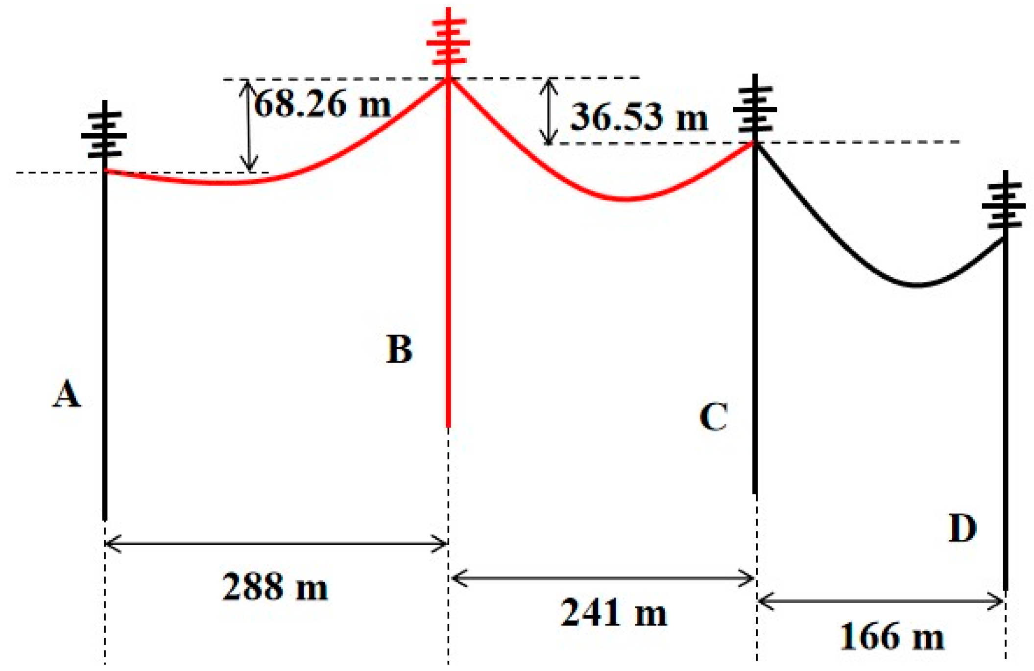
Cup-type towers are common transmission tower types in transmission lines [23]. The cup-type tangent tower B of 110 kV strain section in a heavily iced area is taken as an example. The designed ice thickness of this strain section is 20 mm, and the icing on the transmission line is severe. The altitude of this strain section is more than 1000 m, and the meteorological conditions and geographic environment are relatively harsh. The cross-section is shown in Figure 1. The height differences between the transmission towers A and B and B and C are 68.26 m and 36.53 m, respectively. The span distances are 288 m and 241 m, respectively. The type of conductor is JL/LB1A-300/50, and the type of ground wire is JLB20A-100. According to the on-site investigations and feedback from the operation and maintenance personnel of the power grid, tower B is most vulnerable to the impact of icing. Therefore, the cup-type tangent tower B is taken as an example, and the finite element simulation model is established in COMSOL 5.6 to study the mechanical characteristic parameters of the weak components of the transmission tower.

2.2. Finite Element Simulation Model of Transmission Tower

2.2.1. Model Construction

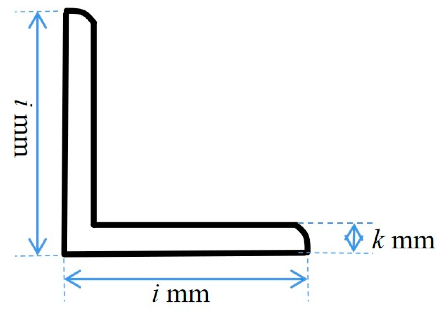
The model utilizes beam elements, comprising 1772 edge elements and 530 vertex elements. Joints are modeled as rigid connections, and the simulation analysis is inelastic. As shown in Figure 2, the members used in the finite element simulation model are equilateral angle steels. The type is designated as Li*k, where ‘L’ represents the shape of the steel, ‘i’ represents the side length in millimeters, and ‘k’ represents the thickness in millimeters. As shown in

Table 1. Cross-sectional areas and applied locations of each type of steel.

Types	Cross-Sectional Areas/cm2	Locations (Marked in Blue)	Types	Cross-Sectional Areas/cm2	Locations (Marked in Blue)
L40*3	2.36		L40*4	3.09
L45*4	3.49		L45*5	4.29
L50*4	3.9		L56*4	4.39
L56*5	5.42		L63*5	6.14
L70*5	6.88		L70*6	7.85
L75*5	7.37		L75*6	8.8
L90*7	12.3		L100*7	13.8
L100*8	15.64		L110*8	17.24
L140*10	27.37

, the cross-sectional areas and applied locations of each type of steel are marked in blue in the corresponding figures.

The main material of the angle steel used for tower B is Q345 steel, and the slant and auxiliary materials are Q235 steel. The material parameters of transmission tower B are shown in

Table 2. Angle steel material property parameters of tower B.

Types	Density/(kg·m−3)	Initial Yield Stress/(MPa)	Poisson’s Ratio	Young’s Modulus/(N·mm−2)
Q235	7850	235	0.3	20,600
Q345	7850	345	0.3	20,600

.

The finite element model of transmission tower B has been established according to the design drawing, as shown in Figure 3.

2.2.2. Loads Application

The self-weight load of the conductor or ground wire G₀ [24] is

$$G_0=m_0{g}_0$$

(1)

where m₀ is the mass per unit length of the conductor or ground wire, g₀ = 9.80665 N/kg.

When conductors and ground wires are covered with ice, the unit ice load is [24]

$$G_i=0.9\pi g_0\left(b_i^2+b_{i}D\right)\times {10}^{-3}$$

(2)

where b_i is the uniform ice thickness of the ice-covered conductors and ground wires, D is the calculated outer diameter of the conductors and ground wires.

The horizontal wind load of the ice-covered conductor and ground wire is [25]

$$G_w=W_0\alpha {\beta }_{\mathrm{c}}{\mu }_{\mathrm{sc}}{\mu }_{\mathrm{z}}{\mu }_{\theta }(D+2b_{\mathrm{i}})\times {10}^{-3}$$

(3)

where W₀ is the standard wind pressure value under the design standard wind speed, α is the wind pressure unevenness coefficient, β_c is the wind load adjustment coefficient of the 110 kV transmission line, μ_sc is the body shape coefficient, μ_z is the wind pressure height changing coefficient; μ_θ is the wind pressure changing coefficient with wind direction caused by the angle between the wind direction and the transmission line axis.

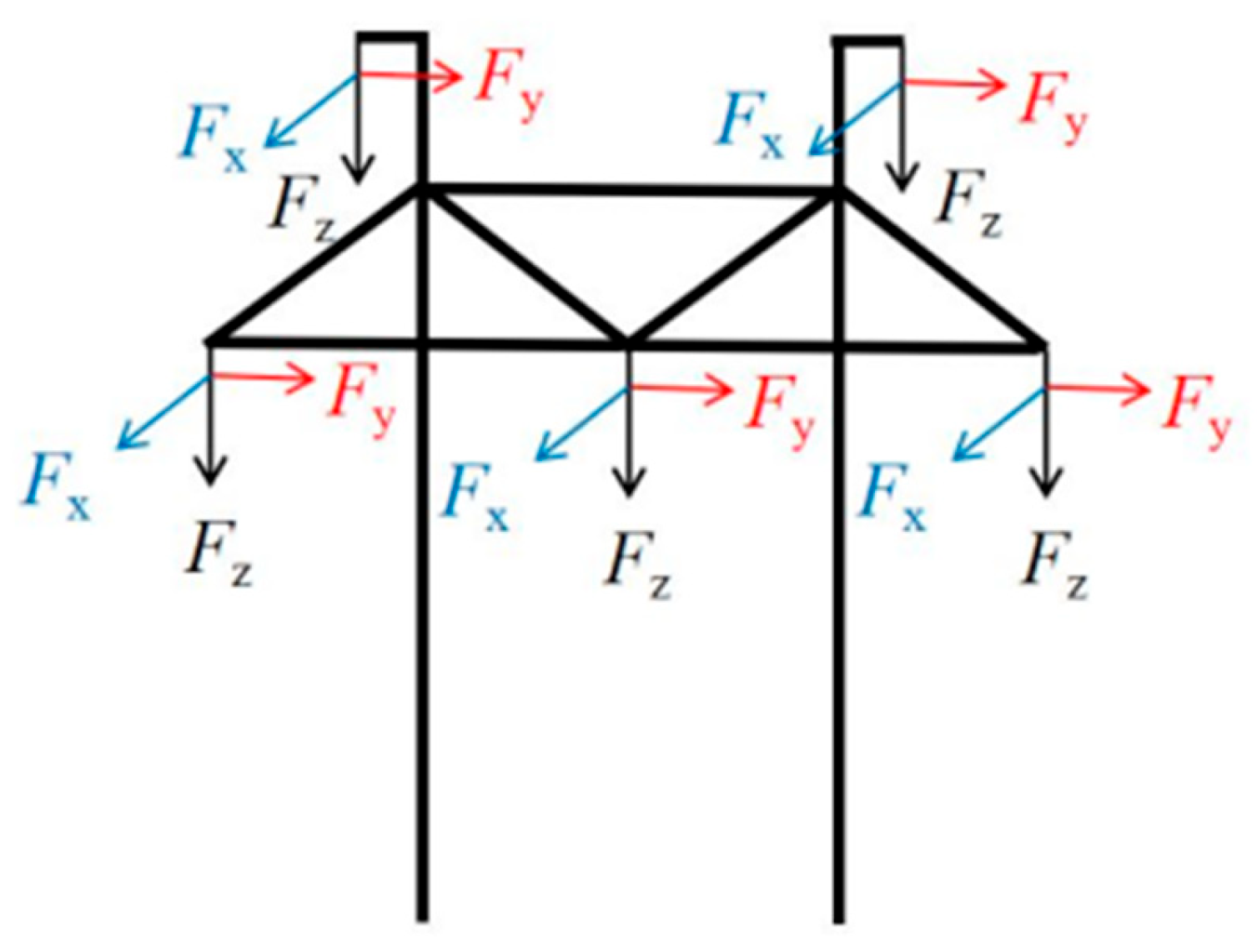
The load borne by the transmission tower includes its own loads and the self-weight loads of the insulators. The insulator string can be regarded as a rigid body, and its self-weight load can be equivalent to the gravity load applied to the transmission tower. In addition, as shown in Figure 4, the loads applied to the transmission tower by the conductors and ground wires include their self-weight load and ice load F_z, horizontal tension F_x, and horizontal wind load F_y, which are equivalently applied to the connection between the conductors and ground wires and the transmission tower [26]. In this paper, the most severe wind load is considered, where the wind angle θ is 90° [27].

The horizontal tension F_x of the conductor and ground wire can be deduced from the approximate formula of the diagonal parabola of the length of the wire [28]:

$$F_x=\sqrt{{\displaystyle \frac{{(G_0+G_i)}^2{l}_0^3\cos {\beta }_0}{24(S-l_0/{\beta }_0)}}}$$

(4)

where l₀ is the span distance, β₀ is the elevation angle, S is the length of the conductor and ground wire.

2.2.3. Example of Simulation Results

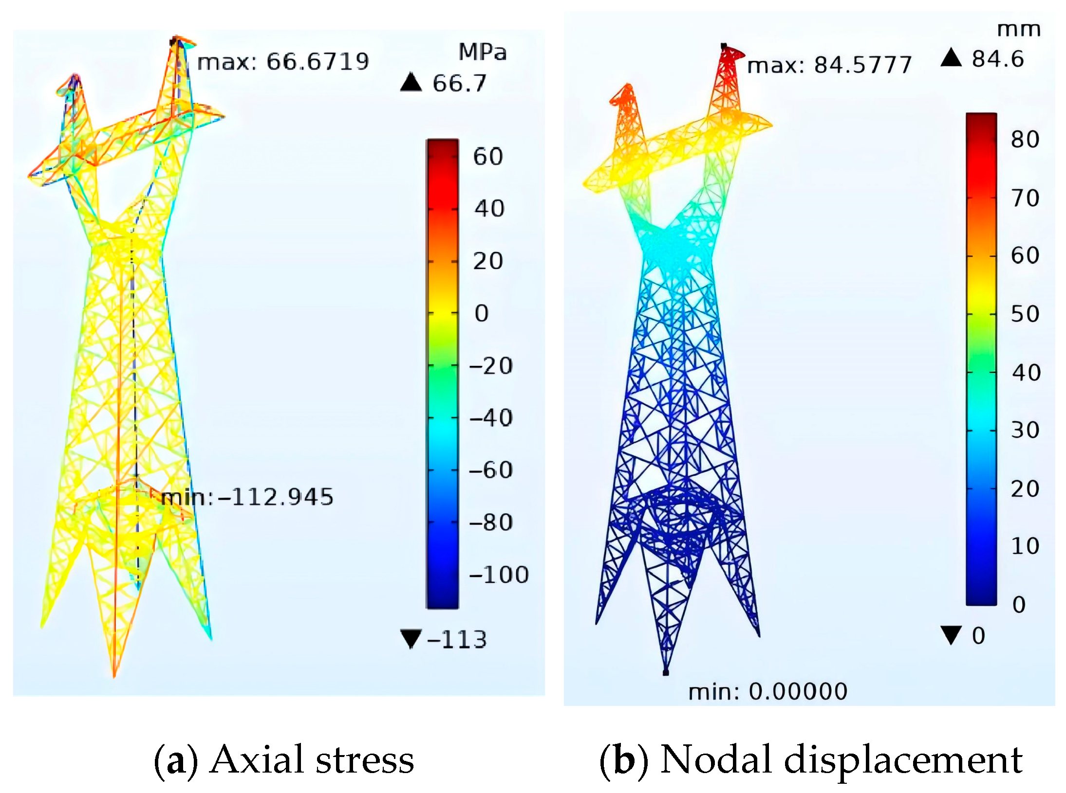
The simulation under Section 2.1 terrain condition with a wind speed of 15 m/s and ice thicknesses of 20 mm on both sides is carried out, at which time the degree of freedom of solving is 5616. The axial stress and nodal displacement cloud images of tower B are shown in Figure 5.

2.3. Input Parameters Are Determined

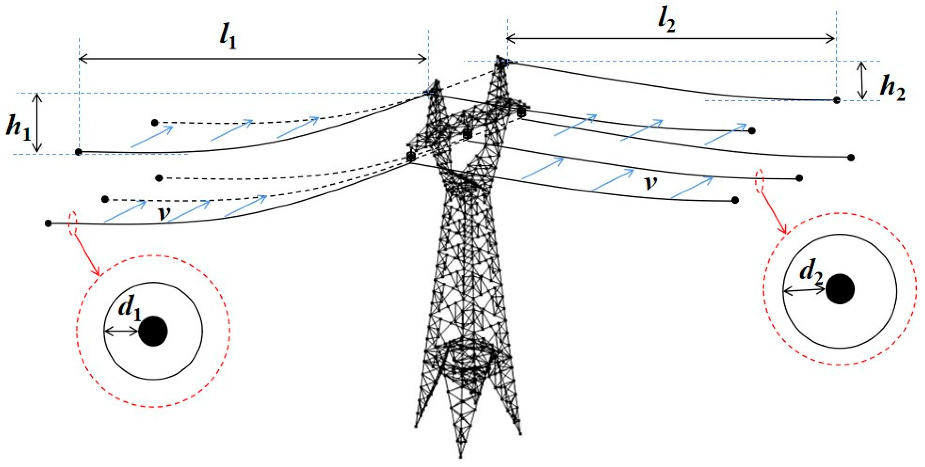
The mechanical characteristics of transmission towers are affected by many factors, such as meteorological and topographical factors. Temperature, humidity, altitude, and other factors are directly related to the ice thickness of transmission lines, and the online monitoring technology of equivalent ice thickness of transmission lines has been widely used in the current power grid [29]. Therefore, based on the consideration of future practical application convenience, these indirect factors are no longer taken into account. Instead, the equivalent ice thickness is considered as one of the influencing factors (i.e., ice thickness referred to as the equivalent ice thickness in this paper) [30]. Existing studies have shown that wind has a large influence on the mechanical characteristics of transmission towers when transmission lines are covered with ice [31,32,33]. Furthermore, the unbalanced tension caused by height difference and span distance may affect the mechanical characteristics of transmission towers [34]. Therefore, seven parameters, including wind speed v, the ice thickness of long-span side conductor and ground wire d₁, the ice-thickness of short-span side conductor and ground wire d₂, long-span side distance l₁, short-span side distance l₂, the height difference of long-span side h₁, the height difference of short-span side h₂, are selected as the input parameters of the finite element simulation model and prediction model of the transmission tower, as shown in Figure 6. The blue arrows represent the wind.

2.4. Weak Locations Analysis of Transmission Tower

The designed ice thickness of tower B is 20 mm, and the designed wind speed is 25 m·s⁻¹. In order to comprehensively obtain the location of the tower’s weak components, the actual topography, climatic conditions, and ice accidents in the area where the transmission tower is located are considered in this paper [35]. The Latin hypercube sampling algorithm is used to uniformly select 500 sampling points in the multidimensional space composed of the range of values of the input parameters, which are used to analyze the location of weak components of the tower. The value range of input parameters is shown in

Table 3. Value ranges of input parameters.

Input Parameters	Symbol	Value Range	Unit
Wind speed	v	[0–26]	m·s−1
Ice thickness of long-span side conductor and ground wires	d1	[0–60]	mm
Ice thickness of short-span side conductor and ground wires	d2	[0–60]	mm
Long-span side distance	l1	[100–350]	m
Short-span side distance	l2	[100–350]	m
Height difference of long-span side	h1	[10–140]	m
Height difference of short-span side	h2	[10–140]	m

.

A total of 500 sets of simulation conditions are conducted in this paper, and some typical sample points are selected, as shown in

Table 4. Part of sample points in 500 sets of simulation conditions.

d1	d2	v	h1	h2	l1	l2	ymax/mm	Location of ymax	fmax/MPa	Location of fmax
0	1	25	58.86	61.94	327	326	52.974	component 1	34.841	component 4
11	11	21	35.88	25.56	276	142	48.256	component 1	29.446	component 3
28	30	11	42.6	28.75	142	125	35.182	component 1	44.327	component 1
36	37	26	37.44	46.2	312	132	104.272	component 1	62.832	component 3
44	47	8	91.8	35.36	306	272	37.929	component 1	59.496	component 1
51	50	1	124.26	50.1	327	167	33.05	component 1	−76.814	component 2

. It is found that the maximum nodal displacement y_max is located at the bracket of ground wire (component 1), and the maximum axial stress f_max is located at the bracket of ground wire (component 1), the connection between the cross arm and the conductor (component 2), the tower body (component 3), and the tower leg (component 4), as shown in Figure 3, in which the locations of the weak components are labeled with red circles.

2.5. Output Parameters Are Determined

The changes in axial stresses and nodal displacements of the weak components of the transmission tower reflect their operational status. The output parameters of the machine learning model are consistent with those of the finite element simulation model, as shown in

Table 5. Output parameters.

Output Parameters	Symbol	Unit
Nodal displacement of the component at the bracket of ground wire	y1	mm
Axial stress of the component at the bracket of ground wire	f1	MPa
Nodal displacement of the component at the connection of cross arm and conductor	y2	mm
Axial stress of the component at the connection of cross arm and conductor	f2	MPa
Nodal displacement of the component at tower body	y3	mm
Axial stress of the component at tower body	f3	MPa
Nodal displacement of the component at tower leg	y4	mm
Axial stress of the component at tower leg	f4	MPa

.

2.6. Mechanical Failure Analysis of Transmission Tower

Based on the above analysis, it is revealed that both wind speed and ice thickness would have certain influences on the nodal displacements and axial stresses of the weak components when the height difference and span distance are determined. Moreover, mechanical failure of the transmission tower may result when the nodal displacements and axial stresses surpass the bearing limits of the key components.

In order to carry out the mechanical failure analysis of transmission towers, here are the steps.

Firstly, parameters such as axial stress f, nodal displacement y of the weak component, and tower height h are collected. Secondly, the stress ratio ξ (the ratio of axial stress f of the main material to its yield stress) of the corresponding steel is calculated. Then, the operational status (Safety Status, Warning Status, Danger Status) of the weak component is obtained with reference to the criteria for transmission towers [26] and the failure assessment criteria given in Ref. [36], as shown in

Table 6. Failure criterion of tower.

Quantization Parameters		Safety Status	Warming Status	Danger Status
Stress ratio	Slant material	ξ < 1.0	1.0 < ξ < 1.15	ξ > 1.15
	Main material	ξ < 0.8	0.8 < ξ < 1.15	ξ > 1.15
Nodal displacement		y < h/1000	h/1000 < y < 3 h/1000	y > 3 h/1000

. When a component is operating in a dangerous state, the operational risk status of the transmission tower is Danger Status. When all the weak components are operating in a safe state, the operational risk status of the transmission tower is Safety Status. In other cases, the operational risk status of the tower is Warning Status. These failure status assessment criteria are more stringent than the actual tower operation status, but they are acceptable in transmission tower mechanical failure assessment.

2.7. Finite Element Simulation Model Validation

• Weak position validation. In this paper, the locations of some weak components obtained by finite element simulation include the bracket of ground wire and the connection of the cross arm and conductor. Ref. [37] provides a case in which the tower head of the same type of tangent tower is damaged due to the ice disaster, and Ref. [38] provides a case in which the cross arm of the same type of tangent tower is broken due to severe icing. The locations of these two accidents are similar to the results in this paper, corresponding to (a) and (b) in Figure 7, respectively.

  Figure 7. Cases of transmission tower damage in the literature. (a) Tower head damage [37]; (b) Cross arm broken [38].

  Figure 7. Cases of transmission tower damage in the literature. (a) Tower head damage [37]; (b) Cross arm broken [38].
• Law validation between wind speed and stress. Huang et al. [39] used fiber-optic grating sensors to carry out transmission tower stress monitoring on a 110 kV experimental transmission line, and the results showed that within the range of wind speed from 0 to 10 m·s⁻¹, the stress of the component at the bottleneck of the tower increased with the increase in wind speed, as shown in Figure 8a. In the finite element simulation model of this paper, the ice thickness is set to 0 mm, and the wind speed increases from 0 m·s⁻¹ to 10 m·s⁻¹. The simulation is carried out at the same position, and the stress of the component at this position increases with the increase in the wind speed, as shown in Figure 8b, which is similar to the test results in Ref. [39].

  Figure 8. Relationships between wind speed and stress at bottleneck of the tower obtained in Ref. [39] and this paper. (a) Results in Ref. [39]; (b) Simulation position and results in this paper.

  Figure 8. Relationships between wind speed and stress at bottleneck of the tower obtained in Ref. [39] and this paper. (a) Results in Ref. [39]; (b) Simulation position and results in this paper.
• Law validation between ice thickness and stress. Li et al. [40] calculated the stress of the main material component at the connection of the cross arm and conductor of a cup-type tangent tower without considering the uneven icing, and the results showed that the stress increased with the increase in the ice thickness, as shown in Figure 9a. In this paper, stress simulation was carried out at the same position under conditions of 15 mm, 20 mm, 25 mm, 30 mm, 35 mm, and 40 mm ice thicknesses. The simulation position and the results are shown in Figure 9b. The stress simulation value of the tower component at the same position also increases with the increase in ice thickness. This result is consistent with Ref. [40].

  Figure 9. Relationships between ice thickness of conductor and ground wires and the stress of the main material at the cross arm obtained in Ref. [40] and this paper. (a) Results in Ref. [40]; (b) Simulation position and results in this paper.

  Figure 9. Relationships between ice thickness of conductor and ground wires and the stress of the main material at the cross arm obtained in Ref. [40] and this paper. (a) Results in Ref. [40]; (b) Simulation position and results in this paper.
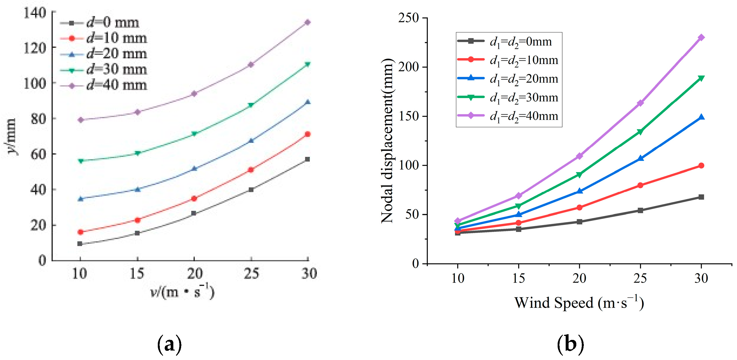
• Comparison validation with another finite element simulation model. Wen et al. [26] took a cup-type transmission tower as an example to establish its finite element simulation model, in which the weak components at the bracket of the ground wire of the tower and the tower body were consistent with some of the weak components of the tower in this paper. The literature simulated 25 groups of conditions with ice thickness of 0~40 mm and wind speed of 10~30 m·s⁻¹ at the bracket of the ground wire of the tower. As shown in Figure 10a, the results show that the nodal displacement of the component at this position increases nonlinearly with the increase in wind speed and also increases with the increase in ice thickness. Moreover, with the increase in ice thickness, the wind speed has a greater influence on nodal displacement. In this paper, consistent height difference and span distance are set to simulate the same position (component 1) and simulation conditions. As shown in Figure 10b, the simulation in this paper obtains that the nodal displacement of component one increases nonlinearly with the increase in wind speed, and the effect of wind speed on the nodal displacement increases with the increase in the ice thickness, which is similar to the conclusion results in the literature.

  Figure 10. The simulation results in Ref. [26] and this paper. (a) Figure of variation curves of nodal displacement y with wind speed v at different ice thickness in Ref. [26]; (b) Results in this paper.

  Figure 10. The simulation results in Ref. [26] and this paper. (a) Figure of variation curves of nodal displacement y with wind speed v at different ice thickness in Ref. [26]; (b) Results in this paper.

In conclusion, by comparing and analyzing the locations of weak components of transmission towers, the relationship between wind speed and tower stress, and the relationship between ice thickness and tower stress with those in the literature and comparing with another finite element simulation model, it can be seen that the finite element simulation model established in this paper is reliable and effective.

3. Data Collection and Prediction Methods

3.1. Data Collection

The training set is required to train the model, and the test set is required to test the model’s training effect in machine learning models [41]. In order to ensure that the input parameters data points are uniformly covered in corresponding value ranges, the Latin hypercube sampling algorithm is used to uniformly and randomly obtain 1200 groups of values as the training set and 300 groups of values as the test set, respectively, within the multidimensional space defined by the value ranges of the seven input parameters. The number of data groups in the training set and test set is determined by the ratio of 8:2 [42]. And then the input data from both sets are substituted into the finite element simulation model in Section 2.2 to obtain 1500 sets of output data.

3.2. Prediction Methods

There is a wide variety of machine learning algorithms; in order to find out the optimal prediction model, five typical regression algorithms, ACO-BPNN, GA-BPNN, SVR, RF, and RBFNN, are used to build regression prediction models.

BP neural network is a multi-layer feed-forward neural network trained according to an error backpropagation algorithm, with self-regulating learning capabilities and the ability to approximate arbitrary nonlinear mapping relations [43]. However, it is easy to fall into the local minimum, which makes it difficult to obtain the saturation area of the global optimum value, which leads to long training time and slow convergence. In order to solve these problems, many improved algorithms have emerged, such as ACO-BPNN and GA-BPNN algorithms.

The ACO-BPNN algorithm is a machine learning algorithm that combines the ant colony algorithm and BP neural network, relying on the principle that ant colonies can find the shortest path to the food location in different environments to improve the model accuracy and stability [44]. Its average error in predicting the coal ash melting temperature reached 5.98%, and the prediction effect is good [45].

The GA-BPNN algorithm combines the genetic algorithm and BP neural network to optimize the weights of the BP neural network through the genetic algorithm while using the backpropagation of the BP neural network to continuously adjust the weights and bias for model training and prediction and to achieve better classification and regression prediction [46]. In terms of predicting loans in the electric power industry, it established a prediction model based on the experimental results of the investment trend of investment funds in the electric power industry over the last 20 years of a bank, which can obtain a prediction error of less than 10% and can accurately fit the investment change curve in the fitting process of the regression curve [47].

The SVR algorithm is used to solve regression problems by constructing a hyperplane to fit the training dataset and minimizing the distance of the hyperplane from these data points. It has advantages in handling small samples, nonlinear fitting, and robustness [48]. Its estimation error in the estimation of the wind power system used for prediction is less than 5.13%, with high accuracy and fast prediction [49].

The RF algorithm is a machine learning algorithm based on decision tree integration that can be used to solve regression problems. By establishing multiple decision tree models and averaging or weighted summing their prediction results to obtain the final prediction value, it can deal with high-dimensional data and is not easy to overfit [50]. The maximum mean square error in battery capacity estimation by using the RF algorithm is 1.3%, with low computational cost and high prediction accuracy [51].

The RBFNN regression prediction algorithm is a regression model based on artificial neural networks. It has the advantages of high efficiency, good convergence, and robustness by mapping the input features into a high-dimensional space by linear transformation and regression prediction of the inputs using radial basis functions [52]. Considering climate and pollution influences, the algorithm was used to predict heavy metal concentrations in lakes under arid environments with a correlation coefficient of 0.99, which is a good fit and high prediction accuracy [53].

Based on the excellent prediction ability of these five types of algorithms in regression prediction, the authors attempt to implement the prediction of mechanical characteristic parameters of weak components of transmission towers under ice-covered conditions with the above five classes of machine learning algorithms by using MATLAB R2018b.

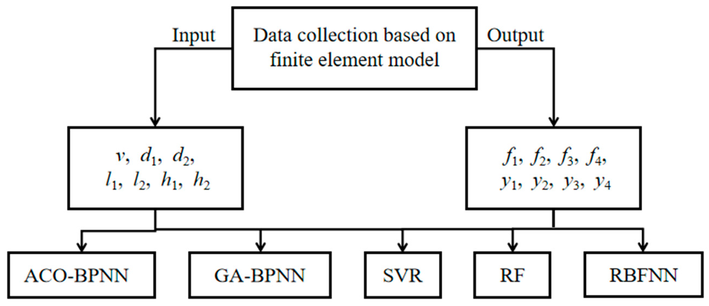
Based on the determined input and output parameters, this study generates seven input and eight output datasets utilizing the finite element simulation model of the tower. These datasets are subsequently employed in ACO-BPNN, GA-BPNN, SVR, RF, and RBFNN algorithms to develop regression prediction models., as shown in Figure 11.

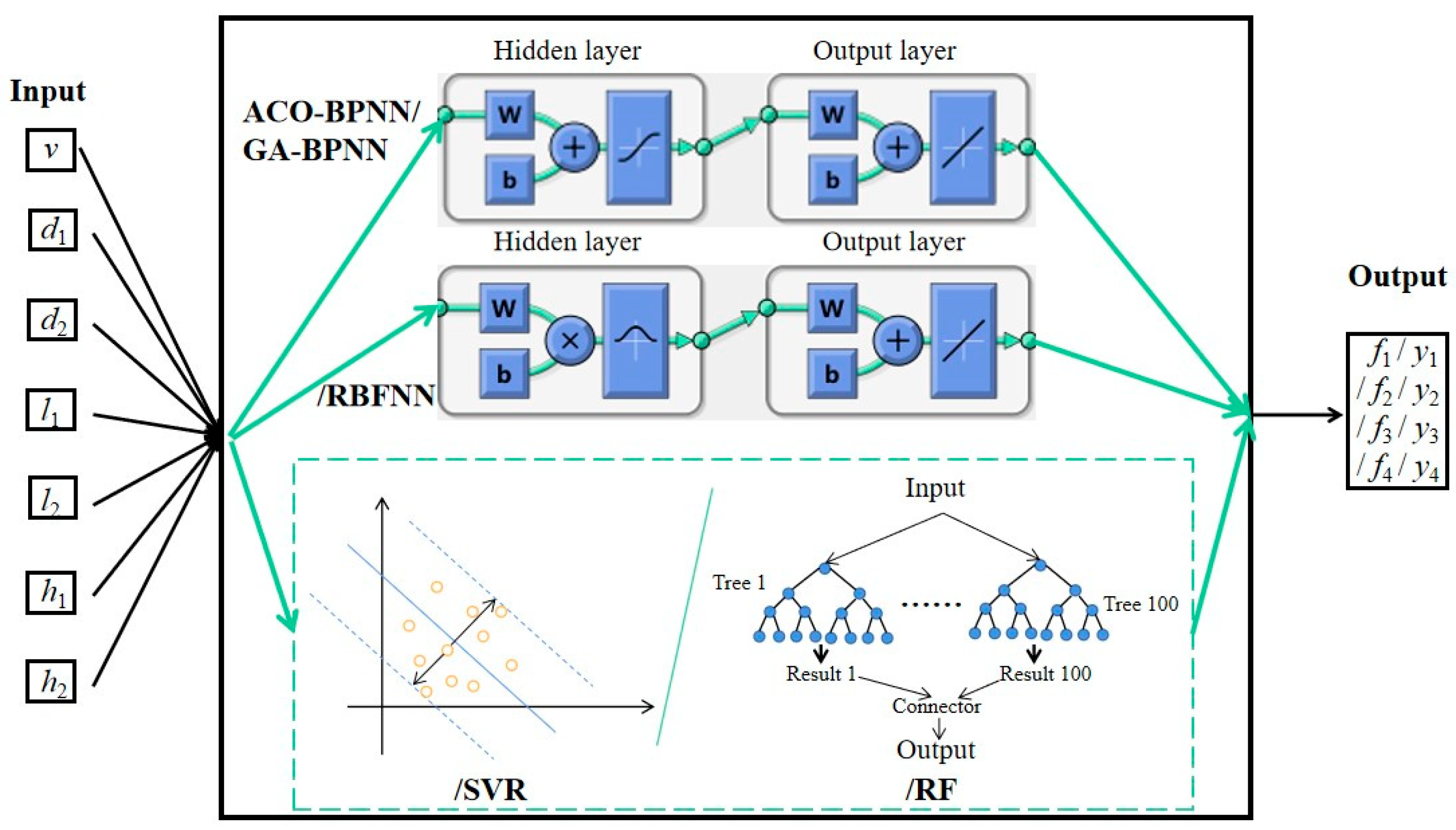
By running the algorithms, it is found that the seven-input/eight-output prediction model takes longer to run than the seven-input/single-output prediction model under the same situation, and the prediction effect is also relatively poor. In order to simplify the model structure and improve the prediction accuracy, eight seven-input/single-output prediction models in each algorithm are established, as shown in Figure 12.

4. Regression Prediction Models

4.1. Data Normalization Processing

In order to unify the value ranges of different features into the same interval, eliminate the quantitative differences between different features, prevent feature weight bias, and accelerate the model convergence speed, each regression prediction model should be normalized for both the training and test sets [54]. The formula is as follows:

$$x={\displaystyle \frac{x_0-x_{\min }}{x_{\max }-x_{\min }}}$$

(5)

where x is the normalized value, x₀ is the original value, x_min is the minimum value, x_max is the maximum value.

4.2. Regression Prediction Model Establishment

The first step in establishing the model is to set the parameters. According to the research results of Robert Hecht-Nielson [55], it has been proven that the structure of a three-layer neural network (including one hidden layer) can approximate and fit any continuous function. Based on this conclusion, a BP neural network composed of a three-layer network structure is selected in this paper, including an input layer, a hidden layer, and an output layer. The number of neurons in the hidden layer is determined by the empirical Formula (6) [56], and the number is set to 12 by manually debugging the algorithm.

$$e=\sqrt{u+w}+a$$

(6)

where u is the neurons number of input layer, w is the neurons number of output layer, a is a constant ranging from 0 to 10.

By adjusting the algorithm hyper-parameters to optimize the prediction results, the hyper-parameters of ACO-BPNN and GA-BPNN regression prediction models are shown in

Table 7. Hyper-parameters of ACO-BPNN and GA-BPNN regression prediction models in this paper.

Hyper-Parameters	Description	Selection of ACO-BPNN	Selection of GA-BPNN
hiddennum	Number of neurons in the hidden layer	12
epochs	Training times	1000
lr	Learning rate	0.01
goal	Minimum error of training objective	0.00001
mc	Additional momentum factor	0.95
min_grad	Minimum performance gradient	1 × 10−6
max_fail	Maximum number of failure times	6
popsize	Initial population size	10	5
maxgen	Maximum generation	50	/
rou	Pheromone evaporation coefficient	0.9	/
p0	Transition probability constant	0.2	/
Q	Total pheromone release	1	/
TF1	Hidden layer transfer function	tansig
TF2	Output layer transfer function	pureline
gen	Genetic algebra	/	50

, and the hyper-parameters of SVR, RF, and RBFNN regression prediction models are shown in

Table 8. Hyper-parameters of SVR, RF, and RBFNN regression prediction model in this paper.

Type	Hyper-Parameters	Description	Selection
SVR	-t	Kernel function type	2
	c	Penalty factor	6
	g	Radial basis function parameter	0.2
RF	trees	Number of decision trees	100
	leaf	Minimum number of leaves	1
RBFNN	rbf_spread	Expansion speed of radial basis function	300

.

4.3. Regression Prediction Model Training

After the hyper-parameters of the five types of regression prediction models are set and the models are constructed, ACO-BPNN, GA-BPNN, SVR, RF, and RBFNN regression prediction models are trained by “train” function, “train” function, “svmtrain” function, “TreeBagger” function, and “newrbe” function, respectively.

The “etime” function is used to obtain the model training time, and the results are shown in

Table 9. Training time of regression prediction models in this paper.

Model Types	Training Time (s)
ACO-BPNN	1742.8
GA-BPNN	576.439
SVR	0.261
RF	2.399
RBFNN	1.073

.

It can be found from Table 9 that the ACO-BPNN model has the longest training time among the five regression prediction models, with a duration of 1742.8 s. In contrast, the SVR model has the shortest training time of 0.261 s.

Even the ACO-BPNN regression prediction model, which has the longest training time, only takes about half an hour to complete the training process. Compared to building finite simulation models and experimental models, machine learning models require much lower manpower and material costs. It takes more time to build the finite simulation model and set up the test platform, while the time for training the machine learning model is relatively less. Thus, machine learning models show great advantages.

4.4. Analysis of Prediction Results of Regression Prediction Models

After training the five types of regression prediction models, the “sim” function, “sim” function, “svmpredict” function, “predict” function, and “sim” function are used to predict the output of both training and test sets, respectively.

• Prediction time analysis

Similarly, the “etime” function is used to calculate the prediction time of different models, and the corresponding outcomes are presented in

Table 10. Prediction time of regression prediction models in this paper.

Model Types	Prediction Time (s)
ACO-BPNN	0.032
GA-BPNN	0.028
SVR	0.062
RF	0.225
RBFNN	0.136

.

To check for overfitting or underfitting, all models predict a total of 1500 sets of data in both the training and test sets. As shown in Table 10, the GA-BPNN model takes the least time of 0.028 s, while the RF model takes the most time of 0.225 s. In contrast, the finite element simulation model established in this paper takes about 5 s to obtain a set of data results.

The computation time of the machine learning model is much less compared to that of the finite element simulation model, greatly increasing the efficiency of obtaining the mechanical characteristic parameters of the weak components of transmission towers.

2.

Prediction results analysis

The prediction effects of five machine learning models are analyzed below.

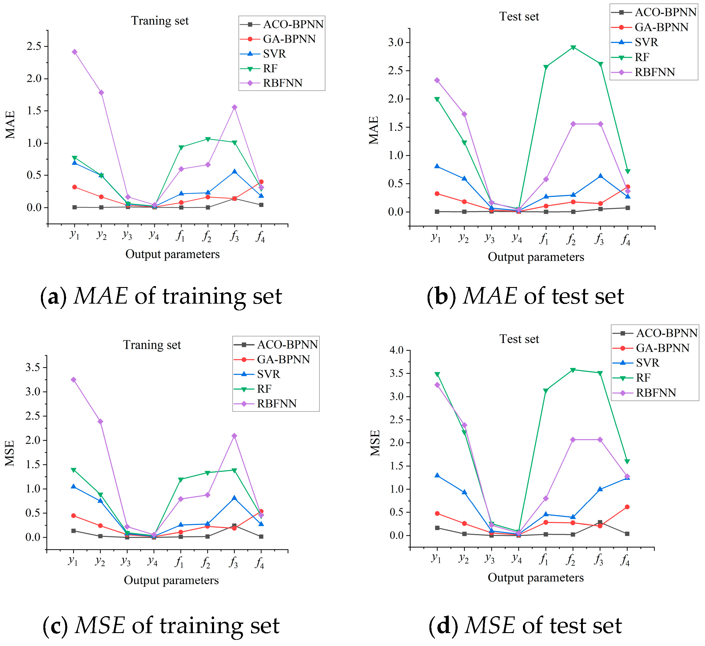
In this paper, MSE, MAE, and R² are used as model evaluation indexes for analysis [17]. MSE is the mean of the sum of the squares of the differences between the predicted and actual values. The smaller the value, the closer the model predictions are to the actual values. MAE is the mean of the absolute value of the difference between the predicted and actual values, and it is also used to measure the proximity of the predicted value to the actual value. The smaller the value, the more accurate the model’s prediction results are. R² reflects the extent to which the independent variable explains the dependent variable and takes values ranging from 0 to 1. The closer R² is to one, the better the model fits the observed data. The specific formulas for R², MSE, and MAE are as follows:

$$R^2=1-{\displaystyle \frac{{\displaystyle \sum {\left(z_i-z_i^{\prime }\right)}^2}}{{\displaystyle \sum {\left(z_i-z\right)}^2}}}$$

(7)

$$MSE={\displaystyle \frac{{\displaystyle \sum {\left(z_i-z_i^{\prime }\right)}^2}}{n}}$$

(8)

$$MAE={\displaystyle \frac{{\displaystyle \sum \left(\left|z_i-z_i^{\prime }\right|\right)}}{n}}$$

(9)

where z_i is the actual simulated value, z_i’ is the model predicted value, n is the number of samples, z is the average value of the actual simulated values.

The R², MSE, and MAE results obtained from the five types of regression prediction models are shown in Figure 13. It was found that

(1)

For the prediction of nodal displacements of the four weak components, the MAE of the ACO-BPNN regression prediction model for the training set does not exceed 0.01 mm, 0.15 for MSE, and R² is not less than 0.999. The MAE of the test set does not exceed 0.01 mm, 0.17 for MSE, and R² is not less than 0.999.

(2)

For the prediction of axial stress of the four weak components, the MAE of the ACO-BPNN regression prediction model for the training set of the model does not exceed 0.15 MPa, 0.25 for MSE, and R² is not less than 0.999, and the MAE of the test set do not exceed 0.06 MPa for MAE, 0.3 for MSE, and R² is not less than 0.999.

(3)

The ACO-BPNN regression prediction model has the smallest MSE and MAE in both the training and test sets and the largest R² among these five regression models, which is approximately equal to one. Furthermore, as shown in Figure 14, there are minimal differences between MSE, MAE, and R² for its training and test sets, indicating no under-fitting or over-fitting. Therefore, the ACO-BPNN model predicts the best results and accurately predicts the mechanical characteristic parameters of the weak components of transmission towers.

In summary, the ACO-BPNN regression prediction model is selected for this paper as the prediction model for the mechanical characteristic parameters of the weak components of the transmission tower.

Figure 13. Evaluation indexes of regression prediction models in this paper.

Figure 13. Evaluation indexes of regression prediction models in this paper.

Figure 14. Comparisons of Evaluation indexes of training set and test set from ACO-BPNN model.

Figure 14. Comparisons of Evaluation indexes of training set and test set from ACO-BPNN model.

To further illustrate the prediction accuracy of the ACO-BPNN model, the comparison results between the simulation results and the prediction results are given in this paper, as shown in Figure 15.

As can be seen from Figure 15, the predicted values of the ACO-BPNN model for the axial stresses and nodal displacements of the four weak components are nearly the same as the simulation values of the finite element simulation model, and the R² for each input parameter is more than 0.999, indicating a high degree of fit and accuracy in prediction results. It further illustrates the accuracy and applicability of the prediction model for mechanical characteristic parameters of weak components of a 110 kV transmission tower, based on the simulation model and machine learning established by using the ACO-BPNN regression prediction algorithm.

5. Case Analysis of Tower Collapse

The 110 kV transmission tower collapse case is taken as an example to illustrate the application effect of the prediction model proposed in this paper.

The transmission tower and conductors were seriously covered with ice due to extreme weather on 3 May 2017, which led to the tower collapse accident. The tower has a total height of 31 m, a designed wind speed of 27 m·s⁻¹, and a designed ice thickness of 20 mm. The span distances of the long-span side and short-span side are 411 m and 406 m, respectively. The ice thickness reached 37 mm, and the instantaneous wind speed reached 27 m·s⁻¹ when the accident occurred [57].

In order to invert this transmission tower collapse case, the data of relevant parameters are used as a group of input data, and the predictions are carried out using the ACO-BPNN prediction model (the optimal prediction model). The simulated and predicted values of nodal displacement and axial stress of each weak component are obtained, as shown in

Table 11. The simulated and predicted values of nodal displacements and axial stresses of weak components.

Types	Simulated Values	Predicted Values	Relative Error between Simulated Value and Predicted Value
y1	171.89	171.87	−0.012%
f1	49.59	49.61	0.04%
y2	120.67	120.69	0.016%
f2	−35.05	−35.01	−0.114%
y3	13.55	13.57	0.148%
f3	111.49	111.44	−0.045%
y4	5.15	5.16	0.194%
f4	56.51	56.48	−0.531%

.

As shown in Table 11, the absolute values of relative errors between the simulated and predicted values of nodal displacements and axial stresses of the weak components are no more than 0.6%, which indicates the prediction model proposed in this paper can accurately predict the mechanical parameters of weak components.

The tower height of the finite element simulation model in this paper is 35.6 m. According to the failure assessment criteria in Section 2.6, when the nodal displacement of the weak component is greater than 106.8 mm, its operation status is considered Danger Status.

As can be seen from Table 11, the maximum nodal displacement of the tower is located at the bracket of the ground wire, with the predicted value of 171.87 mm and the simulated value y₁ of 171.89 mm. In addition, the simulated value of the nodal displacement at the connection of the cross arm and conductor y₂ is 120.67 mm, and the predicted value is 120.69 mm. These values are all greater than 106.8 mm. Therefore, it can be clearly found that there is a dangerous risk for tower operation, which is consistent with the accident described in Ref. [57].

6. Conclusions

Aiming at the lack of research on the prediction for mechanical characteristic parameters of the weak components of transmission towers and the problems of cumbersome steps and high computational time costs of building finite element simulation models, the prediction model for mechanical characteristic parameters of the weak components of transmission towers based on a finite element simulation model and machine learning algorithm has been proposed. The following conclusions are obtained:

(1)

The weak components of the finite element simulation model of the 110 kV transmission tower established in this paper were concentrated in the bracket of the ground wire, the connection of the cross arm and conductor, the tower body, and the tower leg. By comparing and analyzing the results with the experimental and simulation results from previous studies, it has been verified that the finite element simulation model in this paper is reliable and effective.

(2)

Seven parameters, including the wind speed, ice thickness of the long-span side conductor and ground wire, ice thickness of the short-span side conductor and ground wire, long-span side distance, short-span side distance, and height difference of the long-span side and short-span side, were taken as the input parameters, and eight parameters, including the axial stresses and nodal displacements of the four weak components, were selected as the output parameters to establish five typical regression prediction models. R², MSE, and MAE were used to evaluate the models.

(3)

The five types of machine learning models established in this paper for predicting the mechanical parameters of weak components of 110 kV transmission towers spent no more than 30 min on the training process and no more than 0.3 s on the prediction process. The regression prediction model built by the machine learning algorithm spent much less time overall than the finite simulation model and experimental test, which can improve efficiency and save human and material resources. In addition, the ACO-BPNN regression prediction model was the most effective. The MAE of the training set was not greater than 0.15, MSE was not greater than 0.25, and R² was not less than 0.999; the MAE of the test set was not greater than 0.06, MSE was not greater than 0.3, and R² was not less than 0.999.

(4)

The collapse of the 110 kV transmission tower was taken as an example to analyze the prediction effect. The absolute values of relative errors between the simulation and prediction values for nodal displacements and axial stresses of the weak components were no more than 0.6%. The risk status of the transmission tower was determined through the mechanical failure criteria, which was consistent with the fact that the tower collapsed.

The research can provide advanced warnings for predicting failures of transmission towers and references for the operation and maintenance of transmission towers in heavily iced areas. In the future, this study could guide further applications of the online monitoring of transmission conductors.

References

1. Li, B.; Bai, J.; He, J.; Ding, C.; Dai, X.; Ci, W.; Zhu, T.; Liao, R.; Yuan, Y. A review on superhydrophobic surface with anti-icing properties in overhead transmission lines. Coatings 2023, 13, 301. [Google Scholar] [CrossRef]
2. Hu, Y. Analysis and countermeasures for large area accident cause by icing on transmission line. High Volt. Eng. 2005, 31, 14–15. [Google Scholar]
3. Cui, J.; Liu, Y. The analysis of reason of the ice flashover and the countermeasure for transmission line insulator. High Volt. Eng. 2004, 30, 60–61. [Google Scholar]
4. Wang, S.; Jiang, X.; Sun, C. Study status of conductor galloping on transmission line. High Volt. Eng. 2005, 31, 11–14. [Google Scholar]
5. Haamidh, A.; Sivasubramanian, J.; Sakthi, G.S. Vulnerable member assessment of power transmission towers collapsed during Vardah cyclone. Innov. Infrastruct. Solut. 2022, 7, 232. [Google Scholar] [CrossRef]
6. Fu, X.; Li, H. Uncertainty analysis of the strength capacity and failure path for a transmission tower under a wind load. J. Wind Eng. Ind. Aerodyn. 2018, 173, 147–155. [Google Scholar] [CrossRef]
7. Sun, W.; Wang, C. Staged icing forecasting of power transmission lines based on icing cycle and improved extreme learning machine. J. Clean. Prod. 2019, 208, 1384–1392. [Google Scholar] [CrossRef]
8. Li, M.; Dong, J.; Yang, J. Full-scale test for tubular steel tower applied in UHV AC double-circuit transmission Line. Proc. CSEE 2009, 29, 102–107. [Google Scholar]
9. Xia, K.; Hua, M.; Li, F. Structural analysis and testing research for Chinese 1000 kV UHV AC transmission tower. High Volt. Eng. 2007, 33, 56–60. [Google Scholar]
10. Han, J. Full-scale test for cruciform angle tower applied in ±800 kV double-circuit transmission lines on the same tower. Electr. Power 2014, 47, 1–6+29. [Google Scholar]
11. Jiang, R.; Liu, X.Y.; He, S. Analysis of full-scale test and the influence of bolt connection slippage of ±800kV UHVDC transmission tower in heavy ice area. Build. Struct. 2021, 51, 51–57. [Google Scholar]
12. Wen, Y.; Hu, Z.; Mao, X.; Wu, J.; Zeng, H.; Yang, T.; Zhao, C. Comparison for mechanical properties of transmission towers in uniform and non-uniform icing condition under micro-topography. In Proceedings of the IEEE/International Conference on Advanced Electrical Equipment and Reliable Operation (AEERO), Beijing, China, 15–17 October 2021; pp. 1–5. [Google Scholar]
13. Xie, C.; Liu, Z.; Wang, J.; Wang, J.; Cao, H.; Diao, Y. Test research on the wind-tunnel failure of equivalent scale model of transmission tower. South. Power Syst. Technol. 2020, 14, 61–68. [Google Scholar]
14. Zhao, M.; He, B.; Feng, W.; Wang, Y.; Feng, L.; Wang, C. Influence of coupling factors on mechanical property of high voltage transmission tower-line structure under ice loading. Proc. CSEE 2018, 38, 7141–7148+7440. [Google Scholar]
15. Liu, C.; Huang, D.; Zhang, Y.; Yang, G.; Qu, D.; Lv, C. Study on mechanical properties of steel on transmission tower under icing load. Key Eng. Mater. 2018, 773, 255–259. [Google Scholar] [CrossRef]
16. Li, H.; Huang, D.; Xu, Y.; Zhang, L.; Ruan, J. Study on integrated modelling of tower-line system for UHV transmission lines and weak spot distribution of towers. In Proceedings of the 16th Annual Conference of China Electrotechnical Society, Singapore, 22 April 2022; pp. 859–866. [Google Scholar]
17. Yang, L.; Chen, Y.; Mei, L.; Hao, Y.; Li, L.; Huang, H.; Zhang, Y.; Zhang, L.; Yang, L. Prediction method for response characteristics parameters of isolated-span overhead lines after ice-shedding based on finite element simulation and machine learning. Electr. Power Syst. Res. 2024, 229, 110141. [Google Scholar] [CrossRef]
18. Wei, Y.; Gao, X. Transmission line galloping prediction based on GA-BP-SVM combined method. IEEE Access 2021, 9, 107680–107687. [Google Scholar] [CrossRef]
19. Xiong, W.; Yuan, H.; You, L. Prediction method of icing thickness of transmission line based on MEAO. Clust. Comput. 2018, 21, 845–853. [Google Scholar] [CrossRef]
20. Zhang, L.; Ruan, J.; Du, Z.; Huang, D.; Deng, Y. Transmission line tower failure warning based on FBG strain monitoring and prediction mode. Electr. Power Syst. Res. 2023, 214, 108827. [Google Scholar] [CrossRef]
21. Hou, H.; Zhang, Z.; Yu, J.; Wei, R.; Huang, Y.; Li, X. Damage prediction of 10 kV power towers in distribution network under typhoon disaster based on data-driven model. Int. J. Electr. Power Energy Syst. 2022, 142, 108307. [Google Scholar] [CrossRef]
22. Huang, X.; Zhao, L.; Chen, Z.; Liu, C. An online monitoring technology of tower foundation deformation of transmission lines. Struct. Health Monit. 2019, 18, 949–962. [Google Scholar] [CrossRef]
23. Yuan, M.; Shen, X.; Du, Y. Digital intelligent measurement algorithm of inclination for EHV and UHV transmission line tower. High Volt. Eng. 2022, 48, 3001–3011. [Google Scholar]
24. Nian, L.; Yang, L.; Hao, Y.; Li, L.; Mao, G. Forces analysis on key components of 110 kV tangent tower with uniform icing in heavy icing area. Smart Power 2020, 48, 15–22. [Google Scholar]
25. DL/T5440-2009; Technical Code for Designing of Overhead Transmission Line in Medium & Heavy Icing Area. CE Council: Beijing, China, 2009.
26. Wen, Y.; Chen, Y.; Mao, X.; Wu, J.; Fan, Q.; Yang, L. Icing risk assessment and reinforcement measures of 500 kV transmission tower. Electr. Power Eng. Technol. 2023, 42, 250–257. [Google Scholar]
27. DL/T5154-2012; Technical Regulation for Design of Tower Structures of Overhead Transmission lines. CE Council: Beijing, China, 2012.
28. Meng, S.; Kon, W.; Tang, B. Design of Overhead Transmission Lines, 2nd ed.; China Electric Power Press: Beijing, China, 2015; pp. 75–80. [Google Scholar]
29. Yang, L.; Chen, Y.; Hao, Y.; Li, L.; Li, H.; Huang, Z. Detection method for equivalent ice thickness of 500 kV overhead lines based on axial tension measurement and its application. IEEE Trans. Instrum. Meas. 2023, 72, 9001611. [Google Scholar] [CrossRef]
30. Gao, S.; Zeng, C.; Zhou, L.; Liu, X.; Gao, B. Numerical analysis of the dynamic effects of wine-cup shape power transmission tower-line system under ice-shedding. Structures 2020, 24, 1–12. [Google Scholar] [CrossRef]
31. Mohammadi Darestani, Y.; Shafieezadeh, A.; Cha, K. Effect of modelling complexities on extreme wind hazard performance of steel lattice transmission towers. Struct. Infrastruct. Eng. 2020, 16, 898–915. [Google Scholar] [CrossRef]
32. Zhang, J.; Xie, Q. Failure analysis of transmission tower subjected to strong wind load. J. Constr. Steel Res. 2019, 160, 271–279. [Google Scholar] [CrossRef]
33. Xie, Q.; Yang, J. Wind tunnel test and numerical simulation on transmission tower-line coupling system. Power Syst. Technol. 2013, 37, 1237–1243. [Google Scholar]
34. Liu, C.; Xiong, L.; Hu, B.; Chen, H. Analysis and review on the typical failure forms of transmission tower of iced power transmission system in Hunan in 2008. Electr. Power 2009, 42, 37–40. [Google Scholar]
35. Guo, T. Icing disasters and prevention measures of transmission lines in Guizhou. High Volt. Eng. 2008, 34, 2000–2001. [Google Scholar]
36. Yu, D.; Li, Z.; Han, F.; Wang, Z. Reliability analysis on ultra-high voltage transmission tower under wind based on performance. J. Disaster Prev. Mitig. Eng. 2013, 33, 657–662. [Google Scholar]
37. Tang, L.; Zhang, L.; Liu, Y.; Liu, Z. Analysis of icing-caused dynamic collapse of transmission towers in Shaoguan. Guangdong Electr. Power 2008, 21, 12–14+22. [Google Scholar]
38. Bao, Y.; Feng, D.; Zhao, Q.; Zhang, H. Ice-Resistant Design of Transmission Line Towers. Power Syst. Clean Energy 2009, 25, 13–16. [Google Scholar]
39. Huang, X.; Liao, M.; Xu, G.; Zhu, Y.; Zhao, L. Stress monitoring method applying FBG sensor for transmission line towers. Electr. Power Autom. Equip. 2016, 36, 68–72. [Google Scholar]
40. Li, Z.; Yang, J.; Han, J.; Huang, T.; Huang, H. Analysis on Transmission Tower Toppling Caused by Icing Disaster in 2008. Power Syst. Technol. 2009, 33, 31–35. [Google Scholar]
41. Berberich, J.; Köhler, J.; Müller, M.A.; Allgöwer, F. Data-driven model predictive control with stability and robustness guarantees. IEEE Trans. Autom. Control 2020, 66, 1702–1717. [Google Scholar] [CrossRef]
42. Huang, G.; Wu, G.; Yang, Z.; Chen, X.; Wei, W. Development of surrogate models for evaluating energy transfer quality of high-speed railway pantograph-catenary system using physics-based model and machine learning. Appl. Energy 2023, 333, 120608. [Google Scholar] [CrossRef]
43. Jin, W.; Li, Z.; Wei, L.; Zhen, H. The improvements of BP neural network learning algorithm. In Proceedings of the 2000 5th International Conference on Signal Processing Proceedings, Beijing, China, 21–25 August 2000; pp. 1647–1649. [Google Scholar]
44. Dang, J.; Wang, L. Optimization control of hydrogen engine ignition system based on ACO-BP. Int. J. Hydrogen Energy 2021, 46, 38903–38912. [Google Scholar] [CrossRef]
45. Liu, Y.; Wu, M.; Qian, J. Predicting coal ash fusion temperature based on its chemical composition using ACO-BP neural network. Thermochim. Acta 2007, 454, 64–68. [Google Scholar] [CrossRef]
46. Wang, S.; Zhang, N.; Wu, L.; Wang, Y. Wind speed forecasting based on the hybrid ensemble empirical mode decomposition and GA-BP neural network method. Renew. Energy 2016, 94, 629–636. [Google Scholar] [CrossRef]
47. Liu, K.; Guo, W.; Shen, X.; Tan, Z. Research on the forecast model of electricity power industry loan based on GA-BP neural network. Energy Procedia 2012, 14, 1918–1924. [Google Scholar]
48. Chen, Y.; Xu, P.; Chu, Y.; Li, W.; Wu, Y.; Ni, L.; Bao, Y.; Wang, K. Short-term electrical load forecasting using the support vector regression (SVR) model to calculate the demand response baseline for office buildings. Appl. Energy 2017, 195, 659–670. [Google Scholar] [CrossRef]
49. Abo-Khali, A.G.; Lee, D.C. MPPT control of wind generation systems based on estimated wind speed using SV. IEEE Trans. Ind. Electron. 2008, 55, 1489–1490. [Google Scholar] [CrossRef]
50. Demir, S.; Şahin, E.K. Liquefaction prediction with robust machine learning algorithms (SVM, RF, and XGBoost) supported by genetic algorithm-based feature selection and parameter optimization from the perspective of data processing. Environ. Earth Sci. 2022, 81, 459. [Google Scholar] [CrossRef]
51. Li, Y.; Zou, C.; Berecibar, M.; Nanini-Maury, E.; Chan, J.; Bossche, P.; Mierlo, J.V.; Omar, N. Random forest regression for online capacity estimation of lithium-ion batteries. Appl. Energy 2018, 232, 197–210. [Google Scholar] [CrossRef]
52. Jiang, Q.; Zhu, L.; Shu, C.; Sekar, V. An efficient multilayer RBF neural network and its application to regression problems. Neural Comput. Appl. 2022, 34, 4133–4150. [Google Scholar] [CrossRef]
53. Elzwayie, A.; El-Shafie, A.; Yaseen, Z.M.; Afan, H.A.; Allawi, M.F. RBFNN-based model for heavy metal prediction for different climatic and pollution condition. Neural Comput. Appl. 2017, 28, 1991–2003. [Google Scholar] [CrossRef]
54. Nawi, N.M.; Atomi, W.H.; Rehman, M.Z. The effect of data pre-processing on optimized training of artificial neural networks. Procedia Technol. 2013, 11, 32–39. [Google Scholar] [CrossRef]
55. Hecht -Nielson, R. Theory of the back -propagation neural network. In Proceedings of the International 1989 Joint Conference on Neural Networks, Washington, DC, USA, 18–22 June 1989; pp. 583–604. [Google Scholar]
56. Pian, Z.; Li, S.; Zhang, H.; Zhang, N. The application of the PSO based BP network in short-term load forecasting. Phys. Procedia 2012, 24, 626–632. [Google Scholar]
57. Han, B. Cause analysis and emergency treatment of a 110 kV transmission line tower collapse accident. Sci. Technol. Innov. 2018, 7, 115–116. [Google Scholar]
Figure 1. Cross section of tower-line system.
Machines 12 00652 g001
Figure 2. Cross section of the angle steel.
Machines 12 00652 g002
Figure 3. Finite element simulation model of tower B.
Machines 12 00652 g003
Figure 4. Loads applied to tower B by conductor and ground wires.
Machines 12 00652 g004
Figure 5. Simulation cloud images of tower B.
Machines 12 00652 g005
Figure 6. Schematic of the input parameters of the model in this paper.
Machines 12 00652 g006
Figure 11. Data collection and prediction method flow.
Machines 12 00652 g011
Figure 12. Structure of the regression prediction models in this paper.
Machines 12 00652 g012
Figure 15. Scatter plots of the correlation between the simulation values and the predicted values in this paper.
Machines 12 00652 g015aMachines 12 00652 g015b