1. Introduction
Rolling bearings, as critical components of rotating machinery, play a pivotal role in industrial production equipment. Statistics indicate that approximately 45–55% of rotating machinery failures are caused by bearing damage [
1]. Therefore, timely diagnosis of bearing health is crucial for ensuring the continuity and safety of production. Traditional fault diagnosis methods, primarily based on signal processing techniques, are often inefficient and struggle with complex faults. With the widespread adoption of artificial intelligence technology, intelligent fault diagnosis algorithms that integrate signal processing and deep learning are becoming a focal point of research [
2].
In recent years, deep learning technologies have made significant advancements in the field of rotating machinery fault diagnosis. Deep learning models, exemplified by convolutional neural networks (CNN), can automatically capture hierarchical features of data across spatial and temporal dimensions through their multi-layered structures and local perception mechanisms. This capability not only obviates the need for complex manual feature extraction but also addresses sophisticated visual challenges such as image recognition and video analysis [
3,
4]. Consequently, employing signal processing techniques to convert one-dimensional signals into two-dimensional spectrograms can fully leverage the powerful feature extraction capabilities of CNNs, thereby enhancing the accuracy and efficiency of fault diagnosis [
5,
6]. For instance, Ding et al. [
7] proposed a multiscale feature mining method based on wavelet packet energy images and CNN for bearing fault diagnosis. Udmale et al. [
8] utilized the fast kurtogram (FK) algorithm to extract FK under various bearing conditions, inputting them into a CNN to accomplish fault diagnosis and classification. Additionally, Ma et al. [
9] converted vibration signals into two-dimensional time-frequency images and input them into the TLCNN model, achieving end-to-end bearing fault classification.
In the actual operation of equipment, prominent background noise in complex working environments often masks the fault signals of bearings, making it challenging to extract valid information directly from vibration signals. This issue particularly affects the accurate extraction of two-dimensional feature maps, thereby impacting the precision of fault detection and diagnosis [
10]. Consequently, although various algorithms have demonstrated excellent performance under controlled experimental conditions, their performance often significantly degrades in real industrial environments when confronted with high noise interference [
11]. Mishra et al. [
12] proposed a method for diagnosing faults in rolling bearings under slow-speed conditions using wavelet denoising. The wavelet denoising algorithm performs well in time-frequency transformations; however, the selection of the wavelet basis function is challenging during noise reduction, complicating the assurance of denoising effectiveness. Keshtan et al. [
13] employed the empirical mode decomposition (EMD) method for non-destructive diagnostic detection of bearing faults. However, a significant issue with EMD is mode mixing, which can complicate the correct separation of signal components, thereby affecting the noise reduction effectiveness. Variational Mode Decomposition (VMD) is a non-recursive signal processing technique introduced by Dragomiretskiy and Zosso in 2014 [
14]. It not only overcomes the mode mixing issue inherent in EMD but also leverages its inherent Wiener filtering characteristics to achieve improved filtering outcomes [
15]. Since its introduction, VMD has been widely recognized for its minimal endpoint effects, high operational efficiency, and robust noise performance, attracting extensive research interest [
16].
Research on CNN in the field of fault diagnosis primarily focuses on enhancing performance. Although traditional algorithms such as AlexNet [
17], GoogLeNet [
18], and ResNet [
19] excel in diagnostic accuracy, their extensive computational complexity and large model sizes limit their applicability in environments constrained by computational power and storage capacity. Additionally, the increasing number of application scenarios and the complex variety of operational environments have placed higher demands on CNN algorithms [
20]. To address this issue, researchers have developed various model simplification strategies from multiple perspectives, achieving notable success to some extent. Iandola et al. [
21] introduced the lightweight architecture SqueezeNet, which reduces the model size to less than 0.5 MB—510 times smaller than AlexNet—through model compression techniques. Furthermore, it reduces the number of parameters by approximately 50 times compared to AlexNet, while achieving comparable accuracy on the ImageNet dataset. Howard [
22] developed MobileNets using depth-wise separable convolutions, which flexibly balance the model’s speed and accuracy by adjusting two hyperparameters: the width multiplier and the resolution multiplier, to accommodate varying application scenarios and device requirements. Subsequently, Zhang et al. [
23] introduced the ShuffleNet architecture, which incorporates pointwise grouped convolutions and channel shuffling techniques, enhancing network performance while reducing computational complexity and model parameters. The introduction of lightweight CNNs not only enhances computational efficiency and the flexibility of model deployment but also promotes the widespread application of deep learning in the diagnosis of rotating machinery faults. For instance, Yao et al. [
24] proposed a lightweight intelligent diagnostic method for bearing faults based on stacked inverted residual CNN. This method effectively identifies the types and severity of bearing faults in various noisy environments, improves diagnostic efficiency, and reduces dependence on the performance of diagnostic equipment. Subsequently, Luo et al. [
25] designed a lightweight CNN AntisymNet based on the Antisym module, which they combined with a dimension expansion algorithm for fault diagnosis in rotating machinery.
Given the increased complexity of fault diagnosis equipment and the constraints on computational power and storage space in edge devices, this paper proposes a lightweight intelligent fault diagnosis method for bearings based on VMD-FK-ShuffleNetV2. The method enhances the model’s robustness against environmental noise through optimized signal preprocessing techniques, and the optimal lightweight bearing fault diagnosis model is selected through experimental analysis. Initially, the vibration signals are converted into a two-dimensional feature dataset using an improved FK algorithm. Subsequently, this dataset is fed into a CNN for fault identification and classification. By comparing the performance of different models in fault diagnosis tasks, the significant advantages of the lightweight CNN, ShuffleNetV2, in bearing fault diagnosis are validated, successfully establishing an efficient and accurate preliminary bearing fault detection mechanism.
2. Improved Fast Kurtogram Algorithm
2.1. Definition of Fast Kurtogram Algorithm
The FK algorithm, an advanced signal processing technique, has been widely applied in the field of rotating machinery fault diagnosis [
26]. This technique, by calculating the kurtosis of signals across different frequency bands, effectively detects non-stationary features within the signals, such as periodic transient impacts. The advantage of this method lies in its ability to search for optimal combinations of frequency and frequency resolution across the entire frequency band plane, thereby adaptively determining the locations and intervals of non-stationary components [
27].
Multilevel FIR filter banks, structured as binary trees, are the predominant method for rapid frequency band division within FK algorithms. Key steps include the following:
(a) Constructing a set of low-pass filters
and high-pass filters
by frequency shifting a standard low-pass filter
. The specific expression is as follows:
In this equation, the cutoff frequency of the standard low-pass filter is . and can be understood as frequency-shifted versions of by 0.125 and 0.375, respectively. Therefore, the cutoff frequency ranges of and are [0, 0.25] and [0.25, 0.5], respectively.
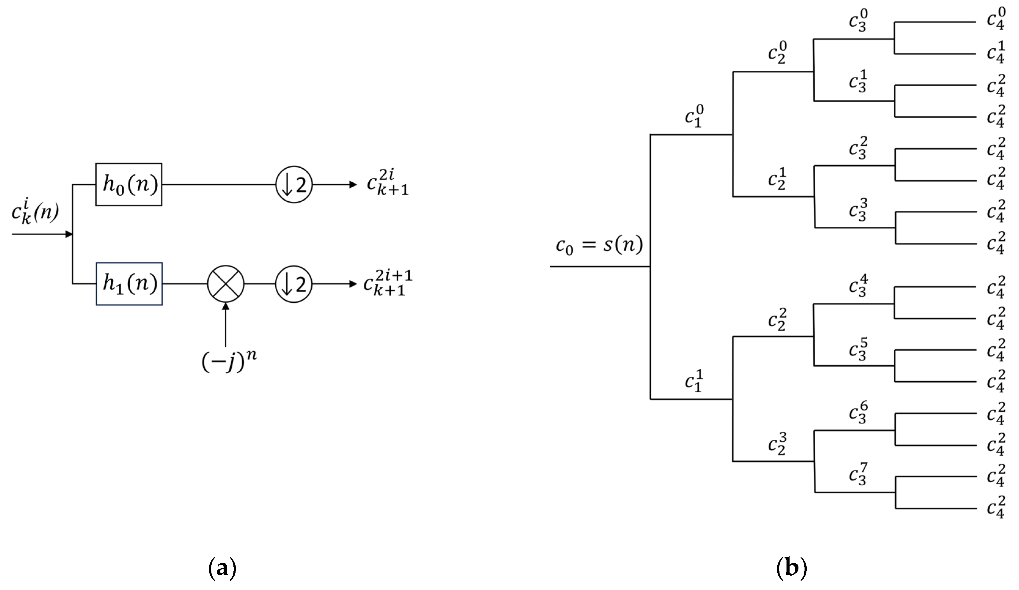
(b) As shown in
Figure 1a, the filters
and
are used for low-pass/high-pass signal decomposition.
represents the i-th decomposition coefficient of the k-th layer, where
and
. After the high-pass and low-pass decomposition of the k-th layer coefficients
, the resulting decomposed signals need to be downsampled by a factor of 2. This produces two new decomposition coefficients,
and
, in the (k + 1)-th layer. To convert the high-pass sequence to a low-pass sequence and maintain frequency order, the sequence filtered by
needs to be multiplied by
before downsampling. The original signal
undergoes low-pass and high-pass decomposition following the binary tree filter bank structure. The tree structure of the FK is shown in
Figure 1b [
28].
The center frequency
and bandwidth
of the decomposed signal
are as follows:
(c)
can be understood as the complex envelope of the filtered signal with
as the center frequency and
as the bandwidth. The kurtosis value of the coefficient
is calculated as follows:
In the equation, and denote the modulus and the mathematical expectation, respectively, and −2 is a constant correction value.
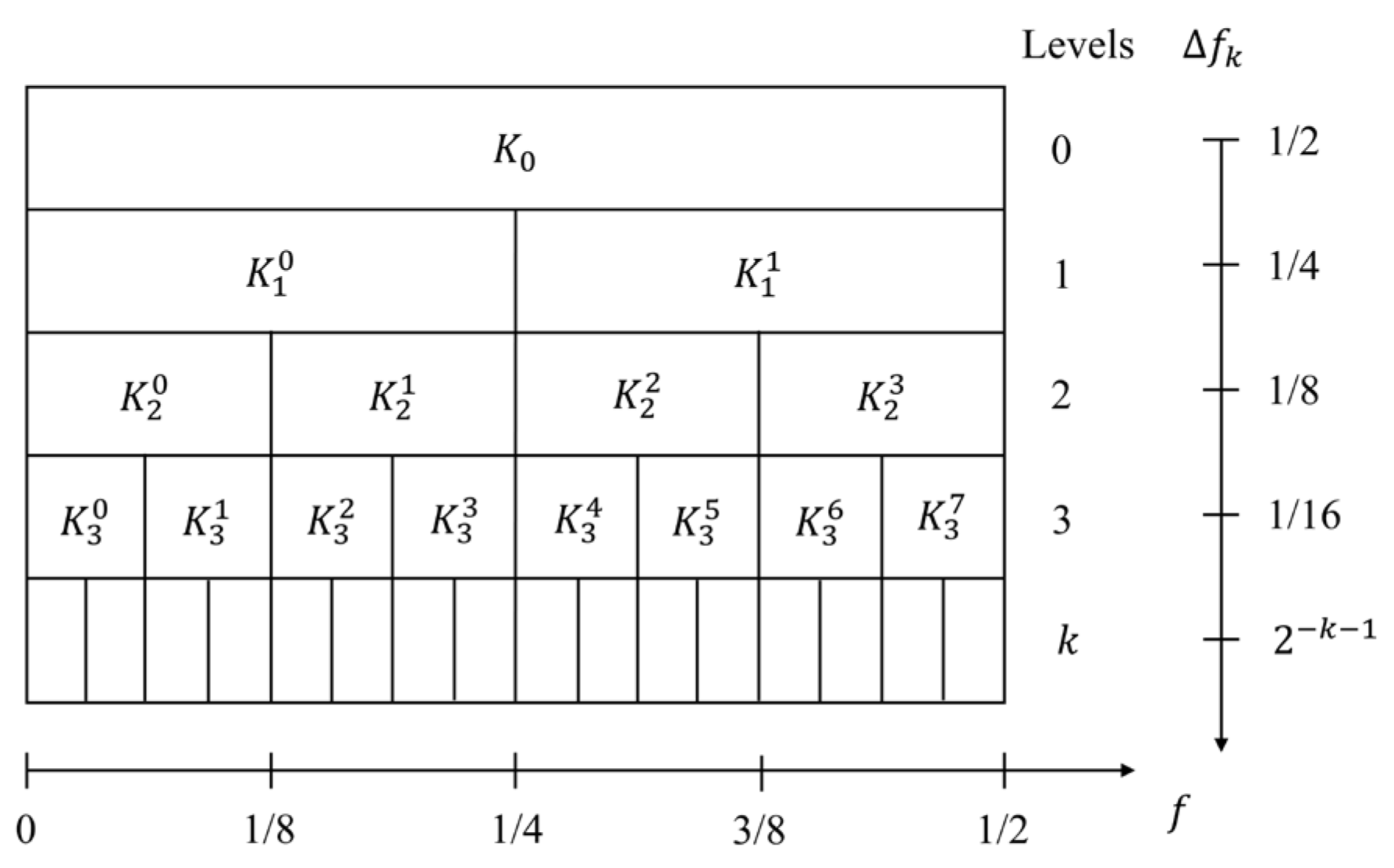
The kurtosis of all envelope signals was calculated, resulting in a kurtosis diagram based on a binary tree filtering structure, as shown in
Figure 2 [
29].
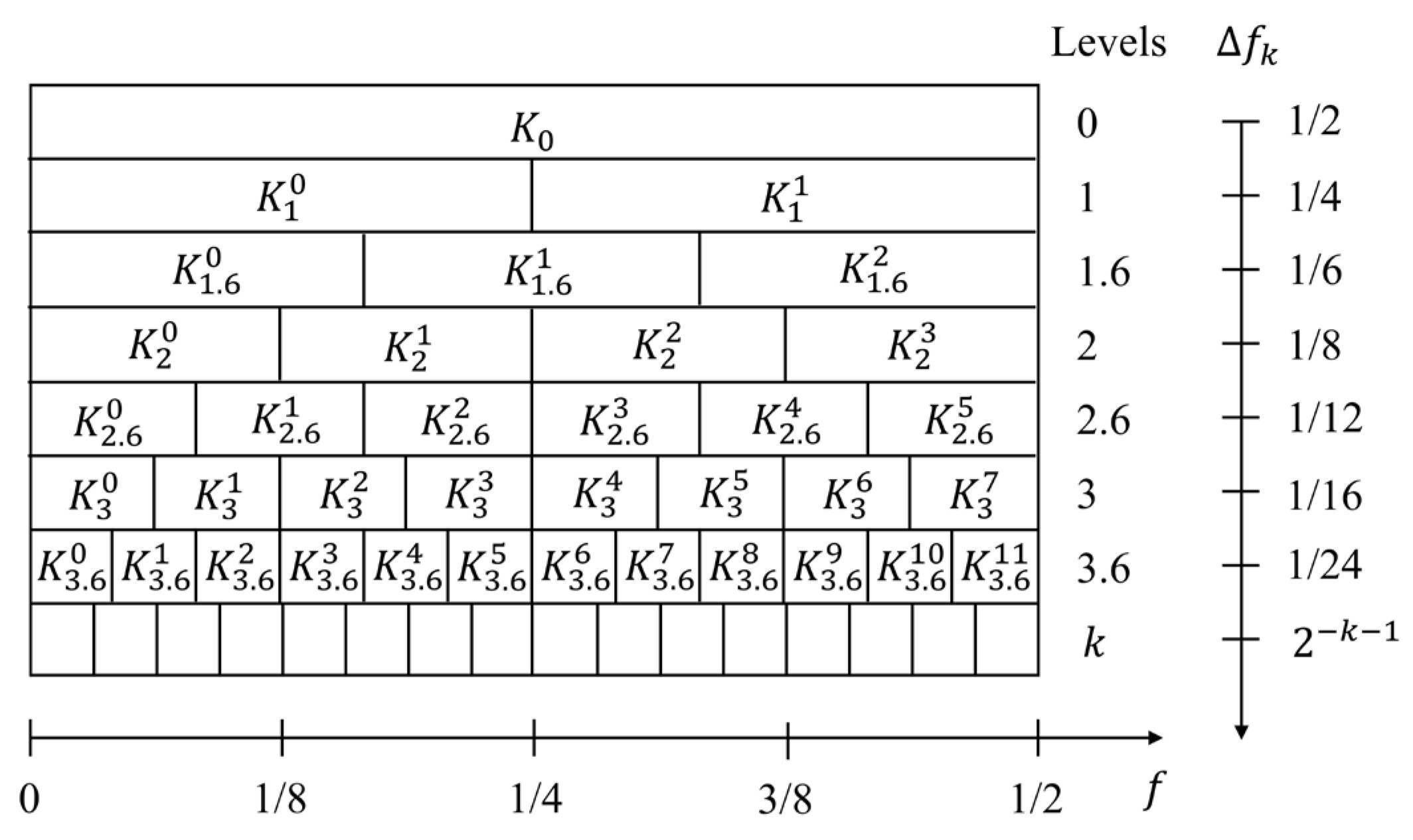
However, the decomposition accuracy of the binary tree structure is low when isolating narrow-band transient impact signals. To enhance the decomposition precision, three quasi-analytical filters with frequency ranges [0, 1/6], [1/6, 1/3], and [1/3, 1/2] were alternately configured with the aforementioned high-pass and low-pass filters. The spectral kurtosis values of the three decomposed frequency band signals were calculated, resulting in a 1/3-binary tree structure fast kurtosis diagram, as shown in
Figure 3.
2.2. Definition of Variational Mode Decomposition
The VMD algorithm, which decomposes the input signal
into
intrinsic mode function (IMF) components through variational analysis, ensures that these components are harmonic signals with limited bandwidth and, as far as possible, non-overlapping frequency bands. The algorithm employs the alternating direction method of multipliers (ADMM) to continually optimize the variational mode model, adaptively searching for the optimal central frequency and bandwidth of each IMF component, thereby minimizing the aggregate estimated bandwidth of the components and effectively separating the signal in the frequency domain [
30]. VMD is a variational problem-solving approach based on three foundational concepts: classical Wiener filtering, Hilbert transform, and frequency mixing [
31]. The specific construction steps are as follows:
(1) Construct the VMD algorithm with constraints. The constraint is that the sum of all intrinsic mode functions equals the input signal
. The goal is to find
intrinsic mode functions
such that the sum of the estimated bandwidths of each mode is minimized.
In the equation, and represent the modal components and the center frequencies, respectively.
(2) Introduce the Lagrange multiplier
and the quadratic penalty factor
to transform the above-constrained problem into an unconstrained one. The quadratic penalty factor ensures the reconstruction accuracy of the signal, while the Lagrange multiplier reinforces the constraints. The expression is given by the following:
(3) In VMD, ADMM is used to solve the above variational problem. By alternately updating
,
, and
, the ‘saddle point’ of expression (7) is sought. The problem of determining
,
, and
in the time domain is converted to the frequency domain, yielding the following solution:
(4) Alternately update
,
, and
until the convergence criteria are met, and then stop the iteration.
Based on the above analysis, the flowchart of the VMD computation is shown in
Figure 4.
During the VMD decomposition process, two core issues are primarily addressed: (1) determining the modal count K, which is the most critical parameter of VMD, and (2) selecting and processing the modes after VMD decomposition. Regarding the determination of the modal number K, this paper uses the total energy difference between the original signal and its decomposed components as a metric. The optimal decomposition level is identified as the K value corresponding to the minimum energy difference [
32]. Additionally, this study employs the Pearson correlation coefficient (PCC) to quantify the correlation between the denoised intrinsic mode functions (IMFs) and the original signal. IMFs with higher cross-correlation coefficients were selected for synthesis, creating a composite signal that encompasses key features of the signal [
33].
In the field of CNN-based rotary machinery fault diagnosis, the FK is commonly utilized as a two-dimensional feature representing faults. However, bearings often contain significant noise during operation, which may interfere with the FK algorithm’s selection of the optimal demodulation band. This interference can result in inaccuracies in the FK, thereby diminishing the diagnostic accuracy of the model. This paper proposes an improved FK method that integrates VMD with the FK algorithm. This approach effectively isolates noise components, significantly enhancing the noise robustness and accuracy of the FK algorithm, thereby improving the capability to extract fault characteristics.
The feature extraction process of the improved FK algorithm is illustrated in
Figure 5:
(1) First, the collected signal is decomposed using VMD. The energy differences of various IMF components are calculated to determine the optimal number of decompositions, K.
(2) Next, the PCC between each IMF component and the original signal is calculated, and the r IMF components with higher correlation are selected for synthesis to obtain the reconstructed signal.
(3) Finally, the FK of the reconstructed signal is extracted using the FK algorithm.
2.3. Validation of the Improved Fast Kurtogram Algorithm through Simulation
To validate the effectiveness of this method, a multi-component simulated signal was designed for experimentation, expressed as follows:
represents a simulated signal of bearing faults, created by superimposing decaying transient sinusoidal waves to emulate the periodic transient impact characteristics caused by faults during bearing operation:
represents an interference signal composed of two low-frequency sinusoidal harmonics:
represents interference from two oscillatory decaying pulses:
To simulate the strong background noise characteristic of bearing faults, noise with a signal-to-noise ratio of −5 dB was added to the simulated signal, expressed as follows:
The simulation signal comprises periodic transient impacts, harmonic components, single-pulse interferences, and Gaussian white noise, authentically mimicking a complex fault environment. The simulation signal was sampled at 30,000 points with a sampling frequency of 10 kHz.
Figure 6 displays the time-domain waveform of the signal and its spectral analysis results. It can be observed from the figure that the signal exhibits significant random fluctuations, with fault information obscured by intense noise interference.
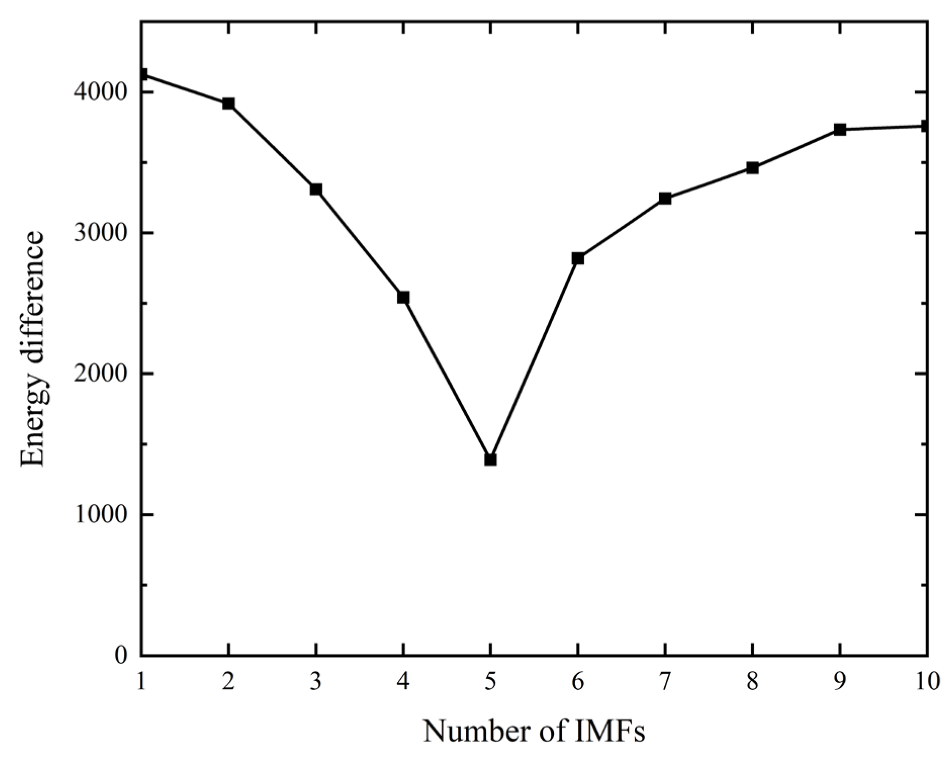
To identify the optimal number of IMF components K in the VMD decomposition process, this study introduced an evaluation metric based on energy disparity. This metric evaluates the decomposition effectiveness by calculating the total energy difference between the simulated signal and all its IMF components. As shown in
Figure 7, experimental results indicate that the minimum energy difference is achieved when the decomposition level K is set to 5. This suggests that VMD decomposition at this level optimally preserves the energy of the original simulated signal, thereby enhancing the precision of signal reconstruction. Consequently, K = 5 is selected as the optimal number of layers for VMD decomposition.
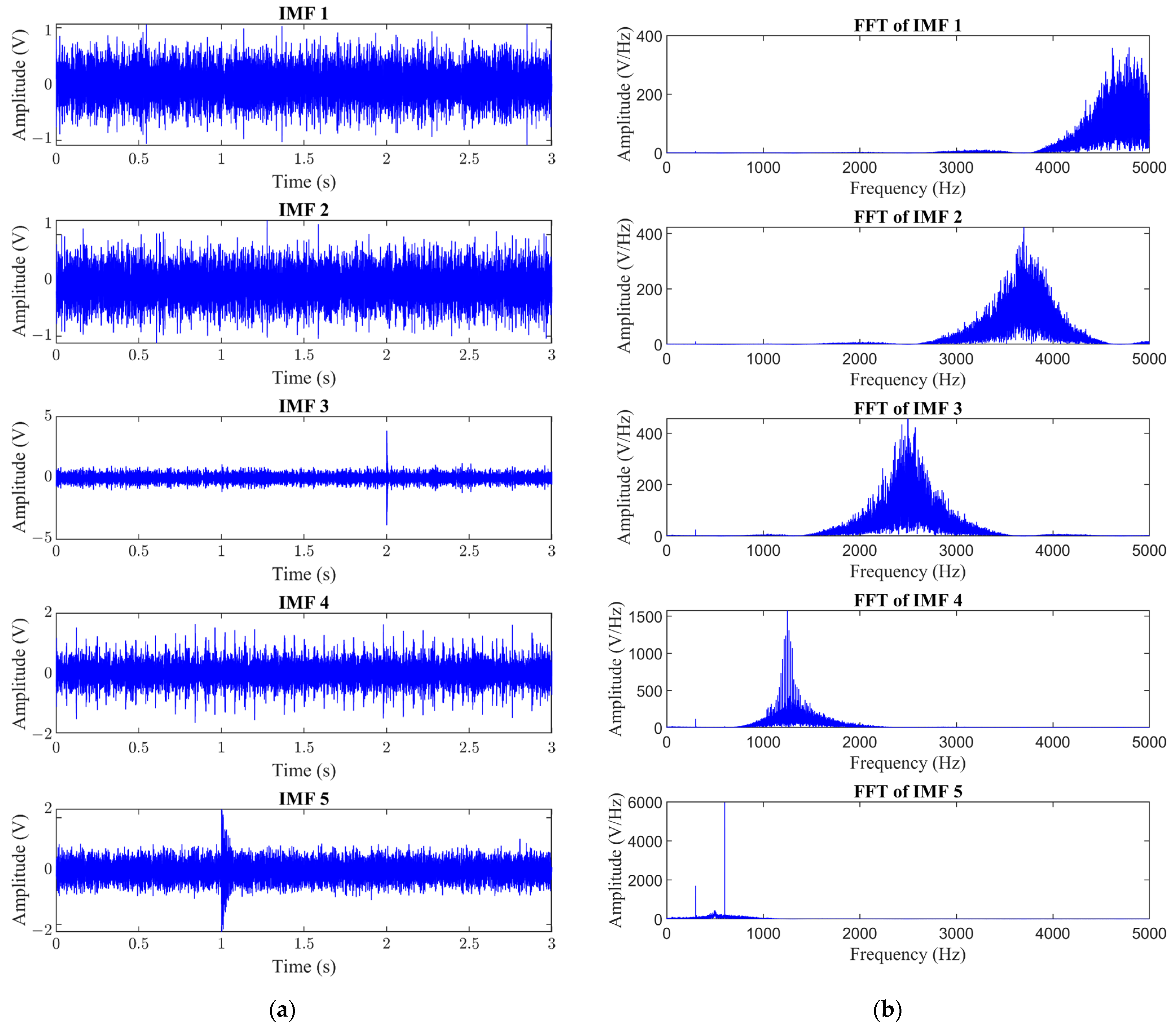
Figure 8 presents the various IMF components of the simulated signal obtained through VMD processing, along with their corresponding frequency spectra. To further quantify the correlation between each IMF component and the original simulated signal, the PCC was computed and detailed in
Table 1. Based on these data, the three IMF components with the highest correlation to the simulated signal (IMF3, IMF4, and IMF5) were selected for signal reconstruction. The reconstructed signal is displayed in
Figure 9. A comparison between the reconstructed signal and the simulated signal indicates, through time-domain analysis, that the reconstructed signal significantly reduces the overall noise level relative to the original simulated signal. It demonstrates higher stability in amplitude, effectively revealing the periodic impact components within the simulated signal. Frequency spectrum analysis results indicate that the denoising process successfully preserved the main frequency components of the signal while effectively controlling high-frequency noise.
As shown in
Figure 10, the results of the original FK algorithm reveal that the optimal center frequency and bandwidth extracted,
and
, are closer to the fundamental frequency of the oscillatory decay pulse interference, 2500 Hz, rather than the desired fundamental frequency of periodic transient impact signals. The bandpass filtered time-domain signal in
Figure 10b does not exhibit clear periodic impacts. The squared envelope spectrum shown in
Figure 10c also fails to accurately extract the characteristic frequencies of periodic transient impacts.
Figure 11 illustrates the results of applying the improved FK algorithm. The optimal center frequency and bandwidth selected by this method are
and
, which are very close to the fundamental frequency of 1250 Hz for the periodic transient impacts in the simulated signal. As shown in
Figure 11b, the filtered signal clearly displays the periodic impact waveform. In the squared envelope spectrum shown in
Figure 11c, the analysis indicates that the amplitude reaches its maximum at a frequency of 16.8157 Hz, which is essentially consistent with the characteristic frequency of 16.67 Hz for periodic transient impacts, demonstrating that the squared envelope spectrum accurately extracts the characteristic frequencies of periodic transient impacts.
The simulation results indicate that, in environments with strong noise and pulse interference, the performance of the traditional FK algorithm is significantly impacted, making it difficult for the FK to accurately filter out the resonance bands associated with faults. In contrast, the improved FK algorithm effectively reduces the interference from noise signals, allowing the FK to more accurately reveal the fault characteristics.
3. Intelligent Fault Diagnosis Method Based on ShuffleNetV2
To validate the efficacy of lightweight networks in bearing fault diagnosis, this study compares three representative traditional CNNs. Specifically, the study analyzes AlexNet, which features a classic streamlined structure; ResNet18, which utilizes residual units; and GoogLeNet, which incorporates Inception modules. Additionally, to fully demonstrate the advantages of ShuffleNetV2 [
34] in bearing fault diagnosis, this study compares it with five other networks employing various lightweight techniques, including SqueezeNet, SqueezeNext [
35], MobileNetV1, MobileNetV2 [
36], and ShuffleNetV1. The core building block of SqueezeNet, the Fire module, evolved from the Inception module. As an enhanced version of SqueezeNet, SqueezeNext introduces multiple levels of Squeeze layers and separable 3 × 3 convolutions, incorporating a residual structure. The core technology of MobileNetV1 involves “depth-wise separable convolutions” to reduce the number of parameters and computational cost. Building on this, MobileNetV2 further optimizes its architecture by incorporating the concept of residual connections from the ResNet framework, introducing inverted residual blocks and a linear bottleneck structure. ShuffleNetV1 integrates “grouped convolutions” and “channel shuffling” techniques, laying the groundwork for the development of ShuffleNetV2. Therefore, the comparative algorithms selected in this paper encompass classic models of both traditional and lightweight networks. Comparative studies confirm the superiority of ShuffleNetV2 and provide a profound analysis of how different lightweight techniques impact fault diagnosis of bearing characteristics, offering both specificity and comprehensiveness [
37].
3.1. Introduction to the ShuffleNetV2 Model
ShuffleNetV2 is an efficient, lightweight neural network architecture developed by Megvii Technology. When assessing model speed, reliance should not solely be on indirect metrics such as floating point operations per second (FLOPs); factors like memory access cost and the level of parallelism must also be considered. ShuffleNetV2 incorporates two principles to optimize network architecture design: first, using direct metrics (such as actual speed) and evaluating on specific platforms; and second, adhering to four specific guidelines for module design. These strategies collectively advance the structural innovation and performance optimization of ShuffleNetV2.
Four guidelines for lightweight network design:
(1) Guideline 1: When the number of input and output feature channels is the same, the memory access cost (MAC) is minimized.
(2) Guideline 2: Grouped convolutions should avoid excessive grouping to reduce MAC and enhance inference speed.
(3) Guideline 3: Network fragmentation reduces network parallelism, affecting the acceleration performance of the graphics processing unit (GPU).
(4) Criterion 4: The memory access and computational time caused by element-wise operations (such as residual summing, ReLU activation, etc.) should not be overlooked.
Under the guidance of the aforementioned design guidelines,
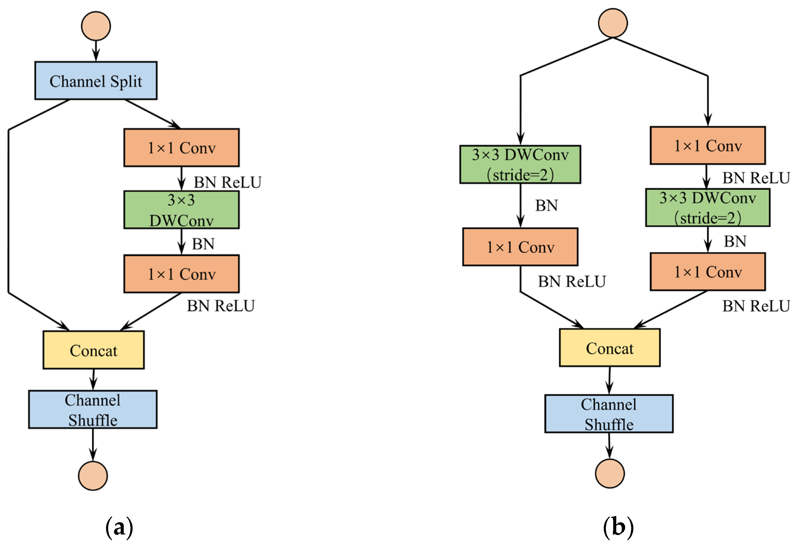
Figure 12 displays the building blocks of ShuffleNetV2. The building blocks utilize a channel split operation, which equally divides the input feature channels into two parts. One part undergoes depth-wise separable convolution to extract deep features, which are then concatenated with the other unprocessed part through a channel concatenation operation. Subsequently, a channel shuffle operation is performed, strategically reorganizing the channels of the two parts of the feature map, breaking the original channel isolation, and promoting inter-channel information exchange. This process significantly enhances the dynamics of the overall information flow of the network, improving its expressive capacity and processing efficiency. In the downsampling module, the channel split operation is omitted; instead, each branch undergoes downsampling with a stride of 2, effectively halving the spatial dimensions of the feature maps and doubling the number of channels. This module design optimizes the use of computational resources of the network, catering to efficient processing demands in resource-constrained environments.
The overall network structure of ShuffleNetV2 is shown in
Table 2.
3.2. Fault Diagnosis Methodology
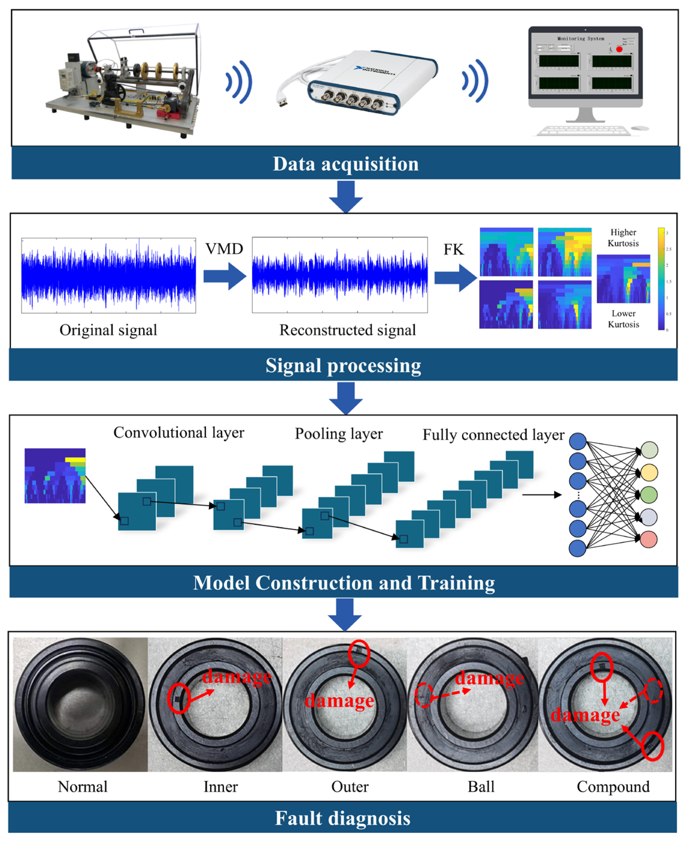
The intelligent fault diagnosis system for bearings based on VMD-FK-Shufflenetv2, as presented in this paper, is depicted in
Figure 13. The diagnostic process encompasses four key steps: data collection, signal processing, model construction and training, and fault diagnosis.
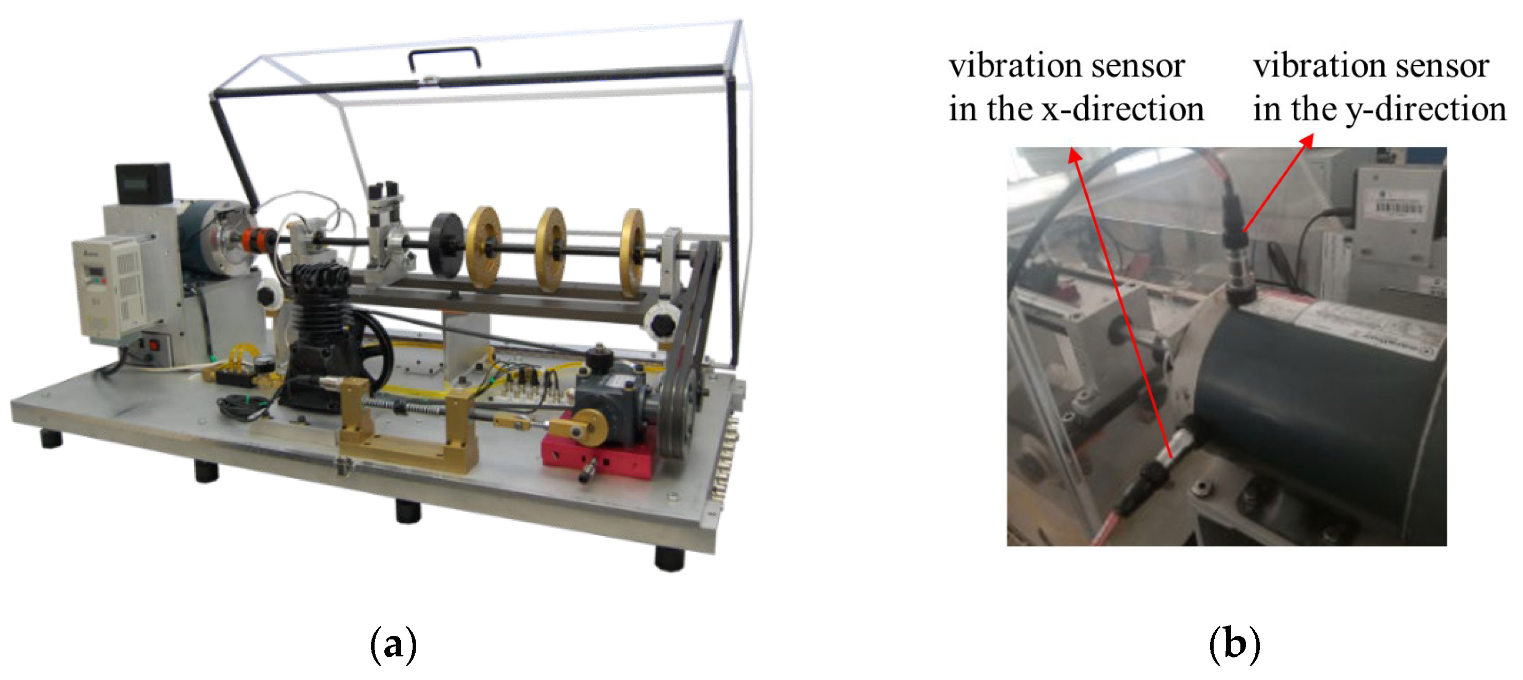
Step 1: Data Collection. Data acquisition forms the foundation of fault diagnosis, as data quality directly affects diagnostic accuracy and reliability. During this phase, vibration sensors are installed on the end cap of the motor shaft in both the horizontal (x-axis) and vertical (y-axis) directions to collect vibration signals. This dual-sensor configuration monitors the vibration characteristics of the equipment from two dimensions, significantly reducing the uncertainty associated with a single measurement point. Additionally, it increases data dimensions and information content, thereby enhancing the comprehensiveness and accuracy of the data.
Step 2: Signal Processing. Signal processing is the core step in the fault diagnosis process, focusing on extracting features highly relevant to the fault state from the signals. In this phase, VMD is initially used to denoise the raw signal. By comparing the energy differences between the raw signal and each decomposed component, the decomposition layer number K with the smallest energy difference is selected. Subsequently, the PCC is used to further quantify the correlation between the denoised IMFs and the raw signal, selecting the IMF components with higher correlation for signal reconstruction. Finally, the FK algorithm is utilized to convert the vibration signals into FK, a method that not only enhances the representation of abnormal signal patterns but also improves the efficiency of pattern recognition.
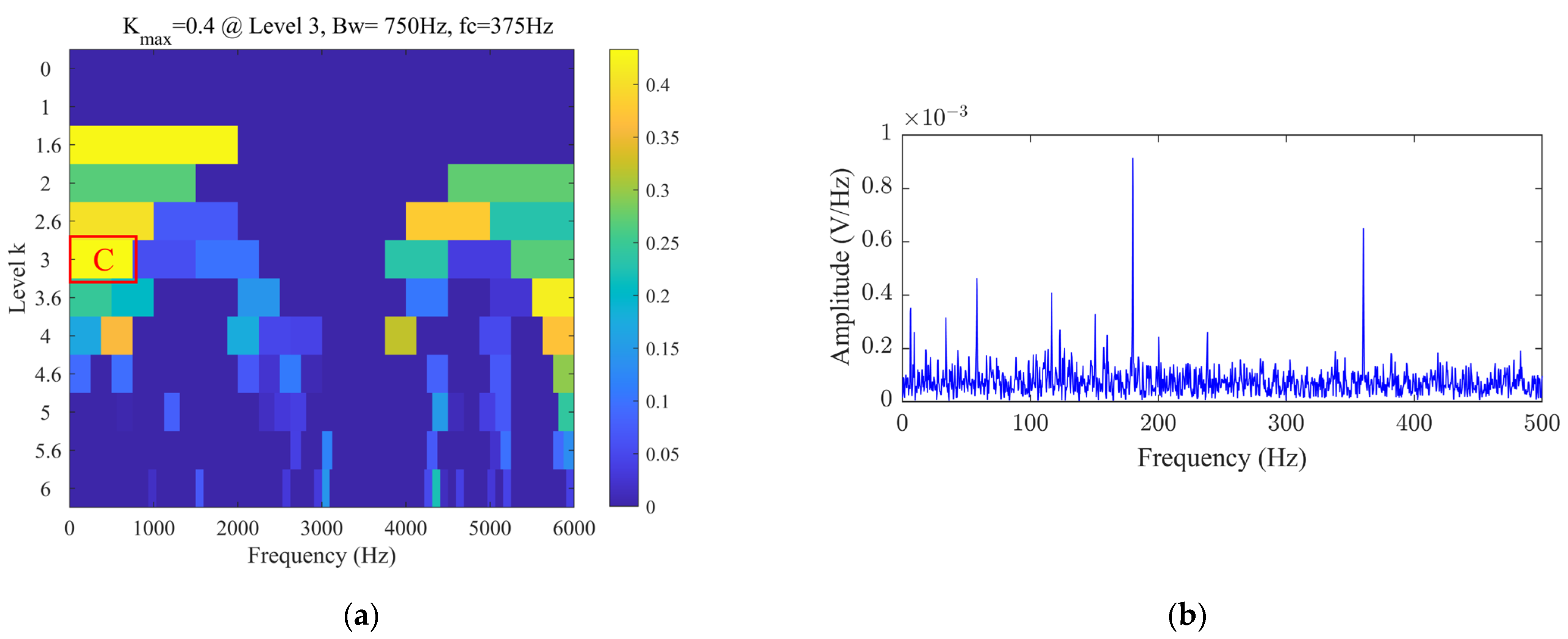
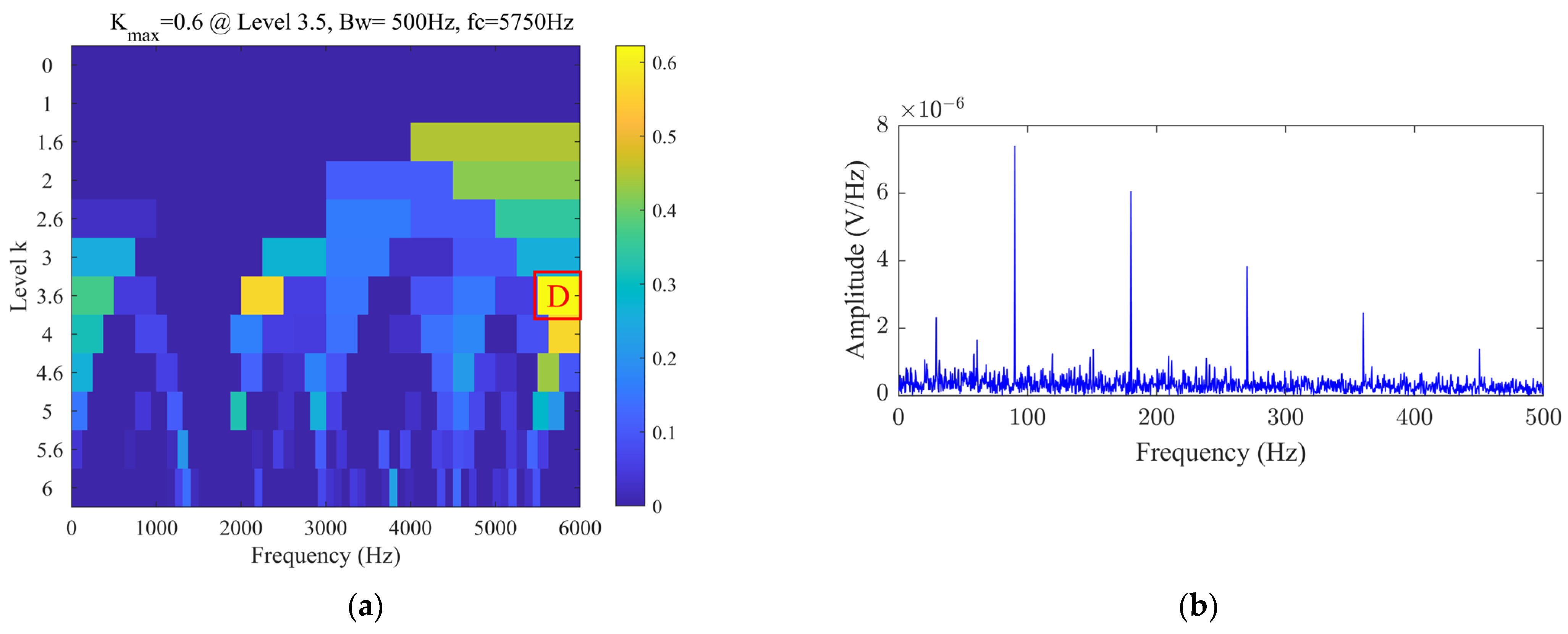
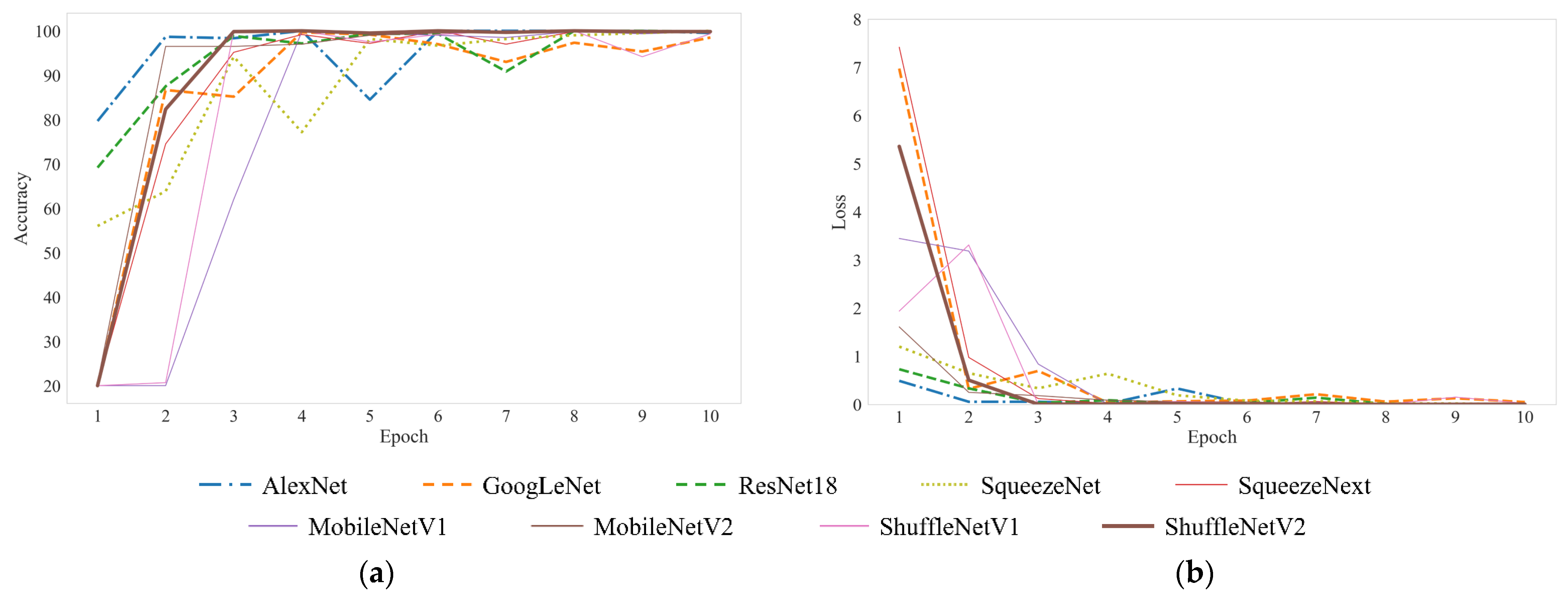
Step 3: Model Construction and Training. The construction and training of neural network models are crucial for achieving intelligent fault diagnosis. Selecting the most appropriate algorithm based on data characteristics, task requirements, and the actual operating environment is essential for effective fault diagnosis. During the model construction phase, the input feature map size of the neural network model is set to pixels to balance performance with resource consumption. For the five types of bearing faults, the output layer of the model is designed with five neurons to meet the requirements of the classification task. During the model training phase, FK data were divided into training, validation, and test sets, which were used for training, validation, and testing, respectively. During the model training process, the training cycles are optimized by real-time monitoring of loss values, terminating the training when the loss values have sufficiently converged. Additionally, a strategy based on saving the best model configuration according to validation accuracy was employed to ensure the accuracy of model selection and its generalization capability. The study constructed three traditional CNNs and six lightweight CNNs, providing a detailed analysis of their performance and training effectiveness.
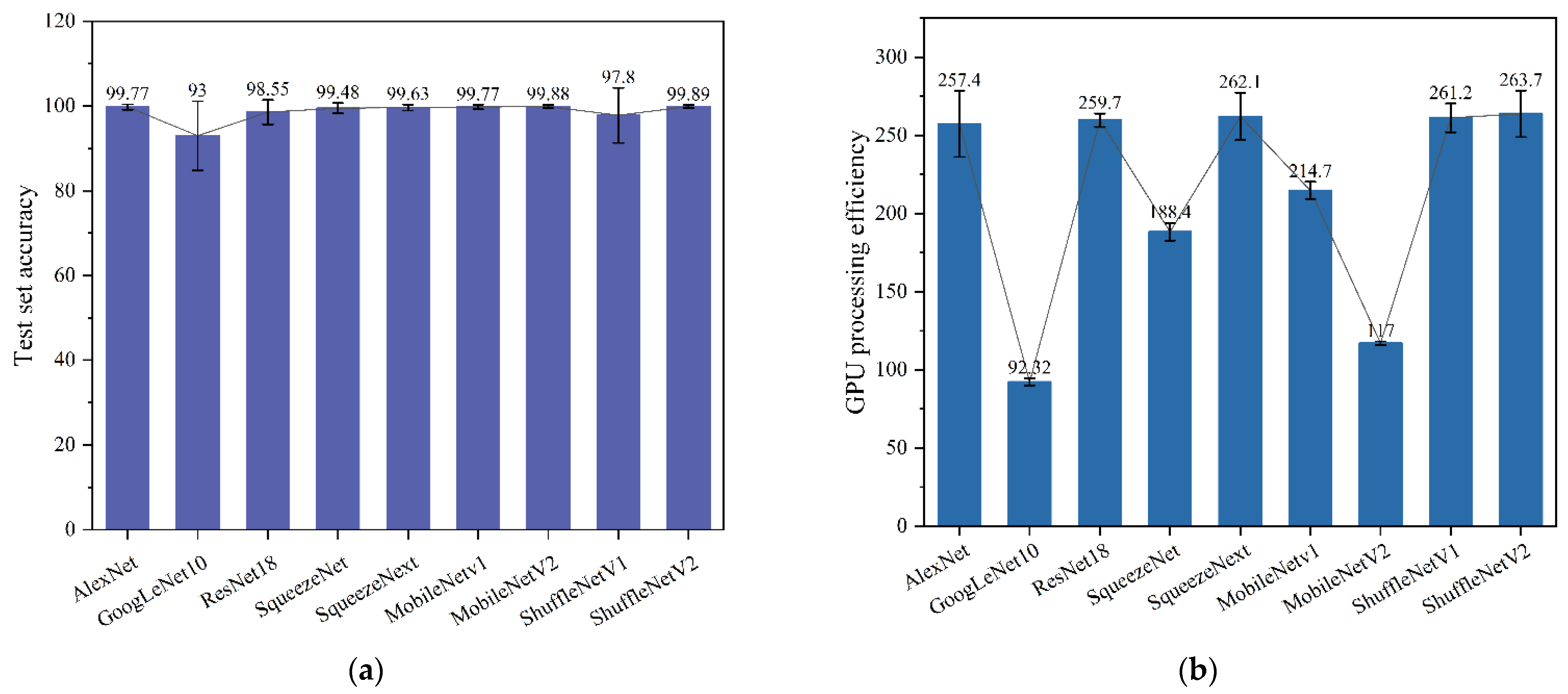
Step 4: Fault Diagnosis. After the training phase is completed, the optimal models saved by each algorithm are used to process the test dataset, performing tasks of identifying and classifying different types of bearing faults. Furthermore, several lightweight metrics and testing performance indicators (such as test accuracy and GPU processing efficiency) are introduced to comprehensively evaluate the performance of traditional neural network models and lightweight neural network models in bearing fault diagnosis.
5. Conclusions
This study introduces a lightweight intelligent fault diagnosis method for bearings based on VMD-FK and ShuffleNetV2, designed to effectively address noise disturbances in bearing vibration signals and to overcome the limitations of traditional CNNs on edge devices with restricted computational resources. The effectiveness of the proposed method was validated through experimental data. The conclusions are as follows:
(1) This study introduces a VMD signal denoising method that integrates energy difference and correlation coefficient, effectively reducing noise levels while preserving critical feature information. Subsequently, the denoised signals were further analyzed using the FK algorithm, and the generated FKs significantly emphasized fault-related features, thereby enhancing the accuracy of fault detection.
(2) Through the assessment of a series of key performance indicators, the study reveals that ShuffleNetV2 outperforms other lightweight and conventional CNN models on a bearing fault dataset. The model not only operates efficiently in environments with limited computational resources but also maintains robust processing capabilities.
The findings of this study highlight the significant advantages of the lightweight intelligent fault diagnosis method for bearings based on VMD-FK-Shufflenetv2 in the field of bearing fault diagnosis. By integrating signal processing techniques with a lightweight neural network model, this method effectively extracts key fault characteristics from complex data, substantially enhancing the accuracy and reliability of fault detection. This establishes a solid theoretical and experimental foundation for the application and expansion of fault diagnosis technologies in resource-limited industrial environments. It holds significant theoretical importance and practical application value in advancing industrial health monitoring systems, particularly in achieving efficient and accurate fault diagnosis and preventative maintenance.
Although the intelligent fault diagnosis method proposed has achieved satisfactory results in preliminary experiments, it still shows limitations in certain areas. Current research focuses primarily on the preliminary diagnosis of bearing faults without delving into diagnosing faults of varying severity or identifying and predicting trends in bearing performance degradation. To overcome these limitations, future research will aim to apply this diagnostic technology to more complex classification and regression tasks, covering areas such as fault severity assessment, health condition evaluation, and remaining life prediction for rotating machinery.
