Abstract
Existing vehicle-road models used for road tracking do not take into account the side slip angle, which leads to a reduction in road tracking accuracy in scenarios where the vehicle is at a large side slip angle, such as an emergency lane change. Consequently, this study presents a path-tracking control technique based on the T-S fuzzy model of heading angle vehicle autonomy. In this paper, based on the yaw angle-based vehicle tracking model, a heading angle-based tracking model considering the side slip angle is constructed. Second, since the vehicle speed varies with time, this paper selects the membership function of the vehicle speed to establish the T-S fuzzy model of autonomous vehicle based on the yaw angle and heading angle, respectively, and ensures the robustness and stability over the whole parameter space by the linear parameter variation robust controller. Then, cost functions based on the yaw angle and heading angle augmented error systems are created separately to optimize the system’s overall performance. Ultimately, simulation and experimentation confirm that the algorithm for control, which is based on the fuzzy model of the heading angle vehicle, has superior autonomous trajectory performance.
1. Introduction
With automobile ownership increasing year by year and problems such as traffic congestion and accidents becoming increasingly severe, the development of traditional automobiles is facing significant challenges [1]. With the integration of the new generation of information and communication, new energy, and other technologies with the automobile industry, the development situation of the world’s automobile industry is facing significant changes. Automobile automatic driving has become the focus and hotspot of research in automobile technology at this stage [2,3]. Automated automobile driving is essential in improving road capacity and reducing traffic congestion [4].
One of the fundamental components of autonomous vehicle driving is the automatic steering system, and the main focus of current research on these systems is trajectory tracking control [5,6]. Since the accuracy of trajectory tracking control correlates significantly with vehicle and road models [7], thoroughly discussing the vehicle-road model is essential. In most vehicle-road models established so far, the heading angle, also known as the yaw angle, is the angle formed by the longitudinal axis of the vehicle and the reference horizontal line. On the other hand, the heading angle, which is the sum of the yaw and side slip angles, is the angle that exists between the vehicle’s traveling direction and the reference horizontal line [8]. When a vehicle is at a large side slip angle, like during an emergency lane change, the accuracy of road tracking decreases since the modeling does not account for the side slip angle’s effect. To help increase path-tracking accuracy, it is crucial to investigate the side slip angle and enhance the vehicle-road model’s accuracy.
Owing to the wheel subsystem’s rapid convergence, a path-tracking model, a friction model in both the longitudinal and transverse directions, and a reduced vehicle motion model based on singular perturbation are constructed [9]. These models are combined to create the final control model. In [10], a path-tracking model is obtained by modeling the dynamics of a four-wheel-independent-steered (4WIS) vehicle and equating the path-tracking problem to minimizing the lateral deviation of the control vehicle concerning the angular deviation of the heading. This paper formulates the vehicle path-tracking task as a constraint-following problem in a novel way [11]. It uses it to represent a model of path-following constraints based on the vehicle model. In [12], an active front steering system’s dynamic model is developed. Unmeasured model perturbations and parameter perturbations in the system are estimated in real-time by introducing a radial-based forward neural network. While the far-precession point model adjusts the steering wheel for anticipated changes in road curvature concerning the lane, the near-precession point model adjusts the steering wheel to estimate the lane center and vehicle state errors. These two steering models are developed independently in [13]. Different models have been developed in the above literature to improve the vehicle path tracking performance, where the heading angle used is the angle between the reference horizontal line and the direction of the vehicle’s longitudinal axis. Still, the actual heading angle is the angle between the vehicle’s direction of travel and the reference horizontal line, and the heading angle is the sum of the yaw angle and the side slip angle [8]. The effect is more pronounced when the vehicle is in a situation with a giant slip angle since this lowers the precision of the vehicle-road model, which, in turn, reduces the accuracy of the route tracking. To improve the accuracy of the model and to study the effect of lateral inclination angle, we propose a vehicle model based on traverse angle and heading angle and draw conclusions by comparing these two models.
Vehicles in the process of driving, vehicle speed, and other vehicle parameters will continue to change, and other elements of the external environment, such as the road surface adhesion coefficient, will also alter. A vehicle two-degree-of-freedom model and nonlinear tires are modeled in [14] with fixed parameters but do not accurately describe the vehicle and the road. Due to the uncertainty in the vehicle’s longitudinal speed and the road friction coefficient, a robust state feedback controller with linear parameters and temporal variation is devised. In the paper, a rectangular polyhedron is built, and the linear matrix inequality (LMI) at the four vertices is solved to realize the feedback gain with different parameter variations [15] Two non-independent parameters, the longitudinal velocity and the reciprocal of the longitudinal velocity, were chosen as variable parameters to design an improved trapezoidal polytope to improve the correlation and to reduce the area of the region in the trapezoidal polytope that is inaccessible to the real state of the vehicle [16]. In order to boost vehicle stability and enhance trajectory tracking precision, adaptive preview times are calculated based on the lateral deviation and road boundaries during vehicle travel [17]. In fact, the modeling of parameter time-varying has been widely studied. In this paper, a T-S fuzzy model is developed for the variation of longitudinal speeds to realize the controller and give the optimal control law at different speeds of the vehicle.
In [18], a fuzzy fast terminal sliding mode control (FFTSM) approach is proposed, which is mainly for multiple-input multiple-output (MIMO) systems. The system state is realized to attain equilibrium more quickly in a finite amount of time by using robust control techniques, and linear matrix inequality (LMI) determines the control parameters. A state feedback controller is suggested in [19] to maintain system performance and stability in the face of time-varying disturbances and system uncertainty. A method of learning-based control for autonomous cars is presented in this research. Using input and output data from an existing controller and the adaptive neuro-fuzzy inference system (ANFIS) method, an explicit Takagi–Sugeno (TS) controller is trained [20]. The hierarchical controller is used, where the upper layer handles the control objectives, the intermediate layer generates the longitudinal slip reference, and the low layer handles the braking of each wheel [21]. In order to provide route tracking control of a vehicle, this study suggests a linear parameter time-varying robust controller. This controller solves the state feedback gain to determine the front wheel steering angle of the vehicle autopilot.
In summary, in order to study the effect of the side slip angle, this paper proposes a vehicle fuzzy model based on the yaw angle and heading angle. It establishes the dynamics and kinematics mathematical models of the two models. On this basis, two robust coordinated control strategies based on the T-S fuzzy model of yaw angle and heading angle vehicles are proposed according to the change in vehicle speed. More effective control schemes are obtained through comparison to improve the accuracy and driving stability of road tracking for autopilot vehicles. The main work of this paper includes the following aspects.
- (1)
- To improve the accuracy of the model and study the influence of the side slip angle on vehicle path tracking, the vehicle path model based on the yaw angle or heading angle is established by taking the line connecting the intersection point of the vehicle traveling direction or body direction and the target path as the origin, respectively.
- (2)
- Aiming at solving the problem of time-varying longitudinal speed of vehicles, the membership function of vehicle speed is selected, the T-S fuzzy model of vehicles is established, and the gain scheduling robust control algorithm considering the variation of the vehicle speed parameter is proposed so as to obtain the optimal control law.
- (3)
- A cost function based on the yaw angle and heading angle augmented error system is defined in order to optimize the system’s overall performance and increase the accuracy of the vehicle path tracking. Additionally, the system’s eigenvalues are limited to a fixed circular region in order to enhance the dynamic performance.
The remainder of this paper is structured as follows. Section 2 presents the T-S fuzzy modeling of vehicle-road systems. Section 3 presents the design of the T-S fuzzy controller. Section 4 and Section 5 validate and compare the two control algorithms through simulation and hardware-in-the-loop (HIL) experiments.
2. Establishment of Vehicle-Road Model Based on T-S Fuzzy Rules
In this section, we present the vehicle dynamics and kinematics model based on the yaw and heading angles. The longitudinal velocity is used as a fuzzy variable to establish the T-S fuzzy modeling of vehicle-road systems.
2.1. Vehicle Dynamics Modeling Based on Yaw Angle and Heading Angle
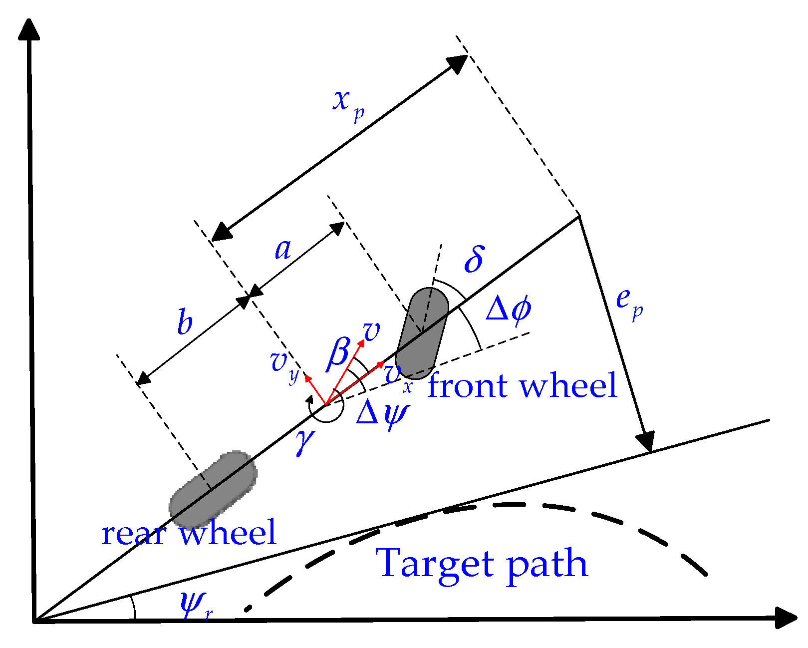
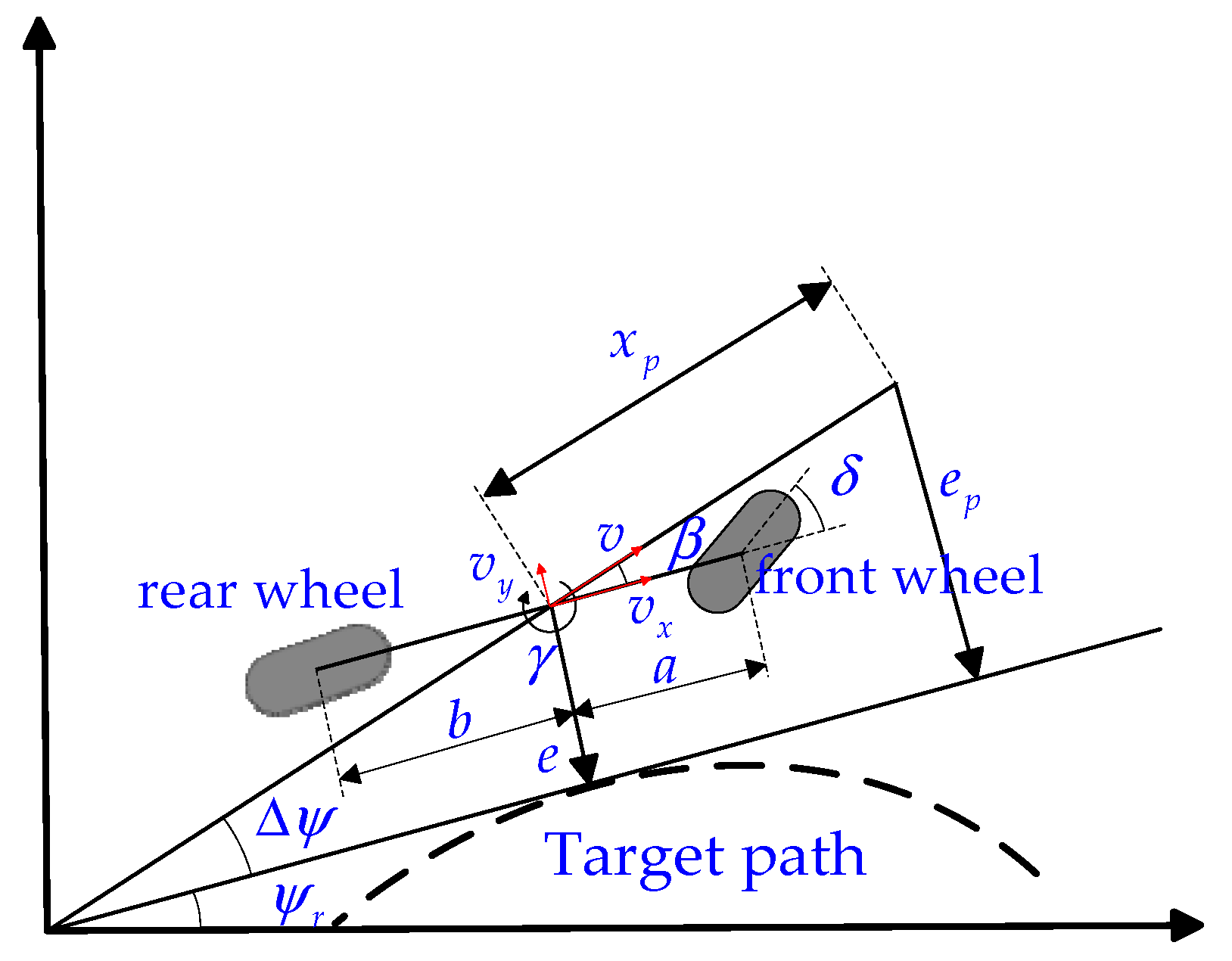
The steering system’s influence is disregarded, the front wheel angle is taken directly as input, the suspension is not taken into consideration, it is determined that the vehicle’s compartment only moves in a planar manner parallel to the ground, and it is assumed that the tire side deflection characteristics are within a linear range, etc., when choosing the vehicle model. On this basis, the vehicle’s two-degree-of-freedom (2DOF) model is selected in this paper. The vehicle dynamics model based on the yaw angle is shown in Figure 1, where the state quantity is the yaw rate, which is the angular velocity in the direction of the vehicle body; it does not take into account the vehicle’s side slip angle. Here, the yaw rate is replaced as the heading rate, and then the heading angle-based vehicle dynamics model is developed, as shown in Figure 2. Figure 1 and Figure 2 show that the vehicle dynamics equations based on the yaw and heading angles can be described as in [22,23,24,25].
where is mass of the vehicle, is the vehicle side slip angle, is the front wheel angle, is yaw inertia of the vehicle, is the vehicle longitudinal velocity, is the vehicle lateral velocity, is vehicle yaw rate, is vehicle heading rate, a and b are the distances from the front and rear axles of the vehicle center of gravity, respectively, and are values of the front and rear tire cornering stiffness, respectively, and the other parameters are defined as follows:

Figure 1.
Schematic of vehicle-road system model based on yaw angle.
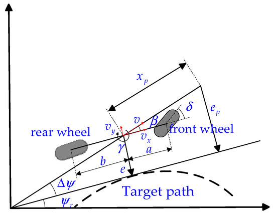
Figure 2.
Schematic of vehicle-road system model based on heading angle.
2.2. Vehicle Kinematics Modeling Based on Yaw and Heading Angles
The lateral deviation of the preview point and the deviation of the yaw or heading angle are selected as the state quantities to guarantee the vehicle’s path tracking, and the vehicle kinematics equations based on the yaw and heading angles are expressed through the dynamics parameters of the vehicle, respectively [26,27,28,29].
The direction of the preview point for the vehicle kinematics equations based on the yaw angle is the vehicle body direction, which can be described as
The simplification by the small angle theorem can be described as
The direction of the preview point for the vehicle kinematics equation based on the heading angle is the direction of vehicle travel, which can be described as
The simplification by the small angle theorem can be described as
where is the vehicle yaw angle, is the heading angle of the reference path, is the pre-scanning distance, and is the road curvature.
Remark 1.
The intersection point of the vehicle moving direction and the target route direction are taken as the origin of the coordinate system in the heading angle-based vehicle-road system model. It takes the heading angle error as the state quantity where the heading angle error is equal to the sum of the yaw angle error and the side slip angle . This accounts for the side slip angle’s influence on increasing the vehicle-road model’s accuracy.
2.3. Vehicle-Road Systems Based on T-S Fuzzy Modeling
Combining (1)–(3), and (5), the vehicle model based on yaw angle and heading angle can be described as
where represents the state vector base on yaw angle, represents the state vector base on heading angle, is the control input, is the disturbance vector, is the measured output base on yaw angle, is the measured output base on heading angle, and the other parameters are defined as follows.
In the process of automobile driving, the longitudinal speed of the vehicle constantly changes to effectively depict the real working conditions of the vehicle in the actual driving, to realize the control system in order to give the optimal control law by judging the current state of the vehicle, and to achieve improvement in the vehicle’s path tracking effect, to take the longitudinal speed of the automobile in the process of driving as a fuzzy variable, and to define i . Then, from system (7), the i rule based on the fuzzy model of yaw angle can be described as [30,31,32].
Control Rule i:
IF v(t) is
Then
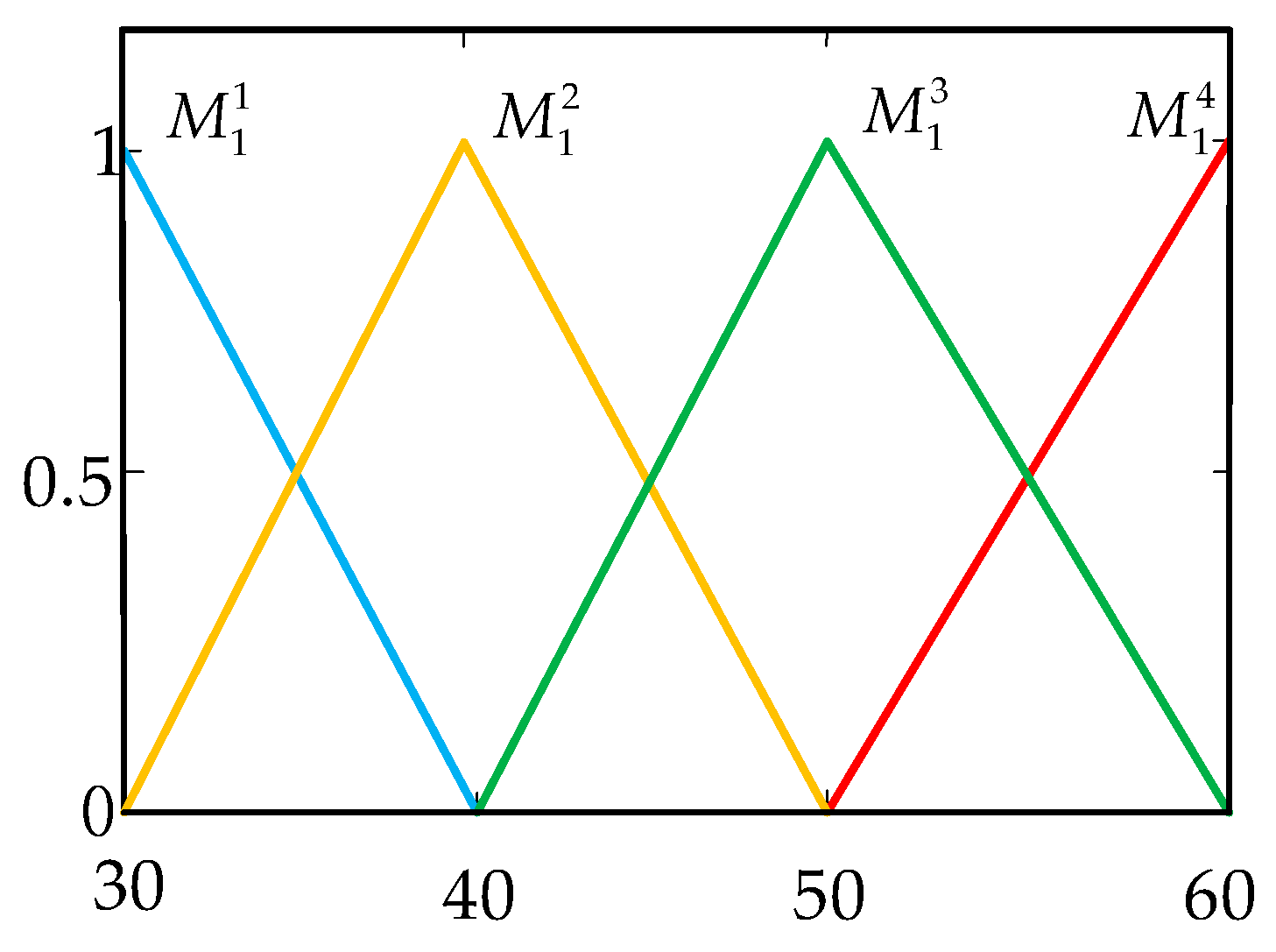
where = are fuzzy variables. The system fuzzy variable is , 40, 50, 60 km/h, where denotes the membership function of v with respect to the fuzzy set [33,34] as shown in Figure 3:

Figure 3.
Membership functions of vehicle speed.
Following fuzzy processing, the yaw angle-based T-S fuzzy system state equation can be obtained, and can be described as [35,36,37]
For any , the following equation holds.
Similarly, the state equation of the T-S fuzzy system based on the heading angle obtained from the system (9) can be described as:
3. Design of Robust Controller Based on T-S Fuzzy Modeling
The path tracking controller for system (10), which is dependent on the yaw angle, can be described as [35]
As a result, the system can be described as
where
Similarly, the system is described by the heading angle-based path tracking controller Equation (14) in the form of Equation (15)
where
Remark 2.
The vehicle-road system based on the T-S fuzzy model takes the longitudinal speed of the vehicle as a variable parameter, and different longitudinal speeds correspond to corresponding feedback gains. The feedback gains in the speed range of neighboring endpoints are solved by the feedback gains of the speeds at the neighboring endpoints with the designed vehicle speed membership function.
In this paper, we consider multiple objectives, including path tracking error, system stability, etc., motivated by the control of the linear quadratic regulator (LQR), and we define the cost function of the system based on the yaw angle augmented error, which can be described as [38,39]
where are the weighting factors and, further, the cost function (16) can be described as
where
The cost function (17) can be equivalently described as
The auxiliary evaluation signal that defines the system based on the cost function can be described as
where
Rewriting the auxiliary evaluation signals yields the final yaw angle-based state system, which can be described as
Similarly, the final state system based on heading angle is obtained, which can be described as
where
Remark 3.

The control objectives are weighted according to the requirements of the control task, and the desired control output is obtained. The matrices , are the weighting matrices which, as shown in Table 1, increases the weights of the lateral deviation and the yaw angle error or heading angle error , where the weight of the lateral deviation is valued more highly to realize the improvement of the path tracking accuracy. To ensure that systems (20) and (21) are stabilized, achieve the control objectives, and satisfy the robust performance requirements, we introduce the following lemmas.

Table 1.
Controller Parameters.
Lemma 1.
For the system that is closed-loop (20), for a given scalar, , holds if there is a positive definite matrix with the right dimension. Following this, the system maintains stability and fulfills the rigorous performance standards for robustness [40,41]. can be described as
Lemma 2.
For the system that is closed-loop (21), for a given scalar, , holds if there is a positive definite matrix with the right dimension. Following this, the system maintains stability and fulfills the rigorous performance standards for robustness. can be described as
Lemma 3.
For D-stability, it is necessary to find a positive definite matrix, denoted as , of suitable dimensions. When Equation (22) is fulfilled, all eigenvalues of this matrix are contained within the region defined by the disk [42].
Due to the influence of the closed-loop system’s state matrix eigenvalues on the controller’s transient response, these eigenvalues undergo scrutiny against the D-stability criterion outlined below, aiming to mitigate transient effects.
Corollary 1.
For D-stability, for the system that is closed-loop (20), when is satisfied, there is a positive definite matrix of suitable dimensions such that each of the matrix’s eigenvalues reside in the disk area. can be described as
The D-stability criterion for the system (20) obtained from Lemma 3 can be described as
The matrix expanded can be described as
The left and right sides of the matrix of Equation (24) are multiplied by the matrix , respectively, to obtain Equation (25), which can be described as
where
The proof of Corollary 1 is completed here.
Corollary 2.
Similarly, for D-stability, for the system that is closed-loop (21), when is satisfied, there is a positive definite matrix of suitable dimensions such that each of the matrix’s eigenvalues reside in the disk area. can be described as
Combining Lemma 1 with the linear matrix inequality (LMI) in Corollary 1, the robust state feedback gain matrix coordinated controller based on the yaw angle fuzzy model can be obtained. Combining Lemma 2 with the linear matrix inequality (LMI) in Corollary 2, the robust state feedback gain matrix coordinated controller based on the heading angle fuzzy model can be obtained.
4. Simulation Setup and Results
This part uses MATLAB/Simulink 2021CarSim 8.02 co-simulation to verify and compare the robust path-tracking control algorithms’ efficacy for the two models presented in this paper.
In MATLAB/Simulink, the fuzzy model of the vehicle is constructed based on the yaw and heading angles. The optimization issue is then addressed for the aforementioned linear matrix inequality (LMI) using YALMIP, a MATLAB toolbox feature. To finish building the joint simulation model, the vehicle’s computed front wheel angle is sent into CarSim, and the state quantity parameters of the vehicle that CarSim produces are fed into MATLAB/Simulink. Table 2 displays the parameter list for the entire vehicle model.

Table 2.
Parameters for an autonomous vehicle.
The maximum permitted deviation for trajectory tracking is one example of the data provided by the literature [35]. Using these parameters, we calculate the weights and of the cost function, as indicated in Table 1, which also includes the pole configuration parameters and the recommended attenuation level.
Using these parameters, by resolving the optimization issue, we obtain the control gains of the two models at the endpoint speeds, and the feedback control gains at different speeds can be obtained by the affiliation function of the vehicle speeds in Figure 3. To confirm whether the controllers, which use fuzzy models for heading and yaw angles, are effective, additional robust controllers based on the yaw angle and heading angle models were added, and the controllers of the four models were evaluated for their performance in the following scenarios: vehicles are subjected to path-following experiments under serpentine and double lane change with high pavement adhesion coefficients at different speeds.
4.1. Serpentine Road Path Tracking
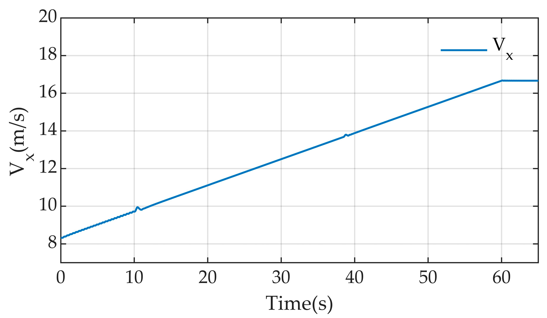
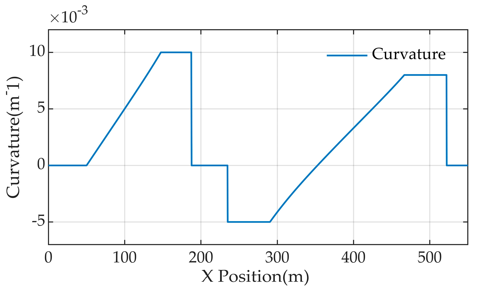
The speed variation of the autonomous vehicle for path tracking on a serpentine road is shown in Figure 4; the speed is increased from the initial 30 km/h, after 60 s increments to 60 km/h, and after that, the speed is uniform. In this paper, the curvature of the target path is selected to change in a certain range, and there is a continuous curve of the serpentine line road. The curvature of the serpentine line road changes, as shown in Figure 5, and the curvature changes in (−0.005, 0.01).

Figure 4.
Vehicle speed changes on a serpentine road.
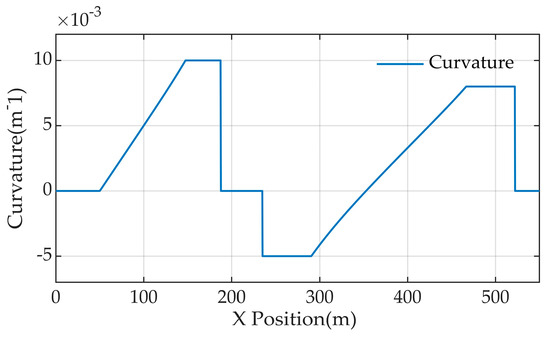
Figure 5.
Serpentine road curvature.
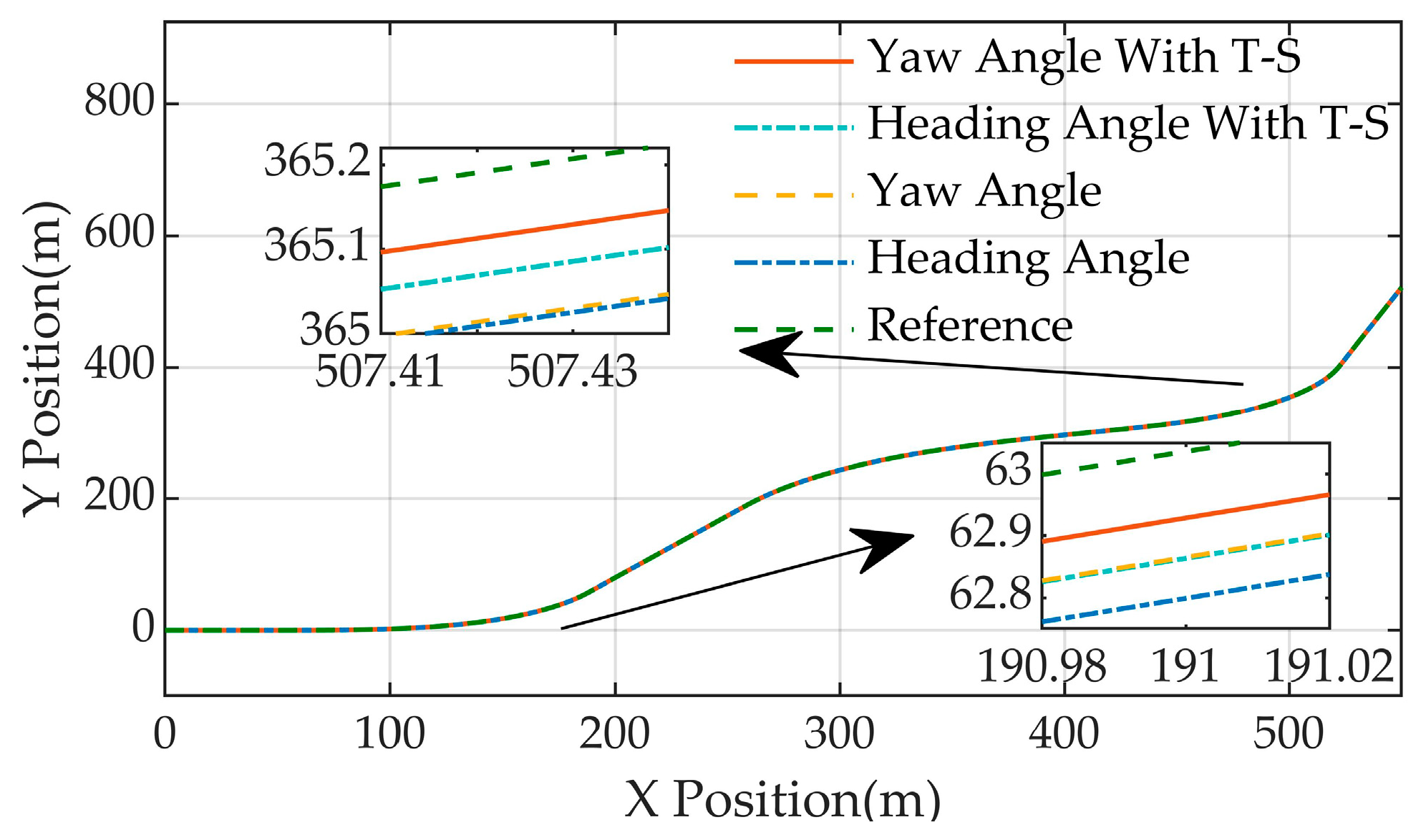
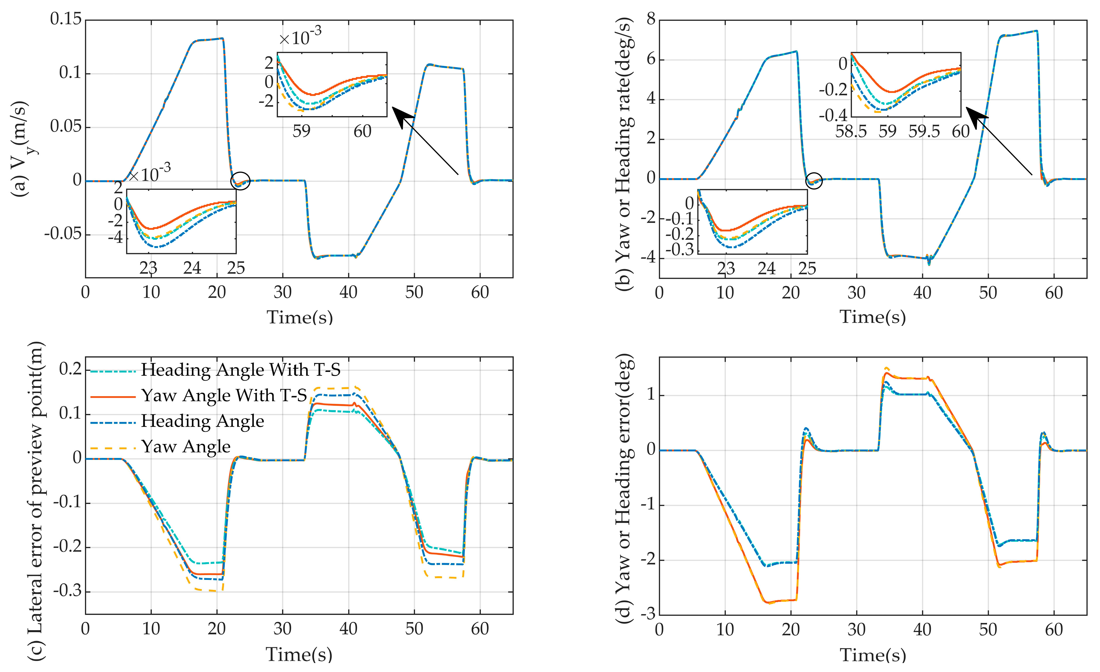
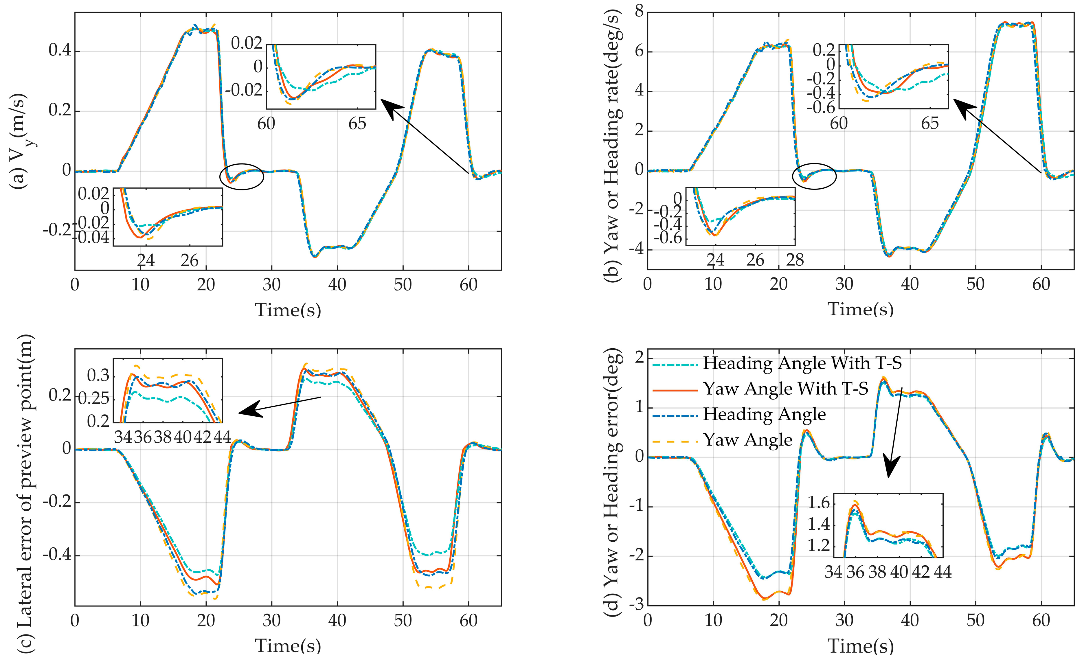
The path tracking and lateral deviation comparison results for the four model control algorithms are given in Figure 6 and Figure 7c. In the figure below the initial end of the arrow shows the position of the corresponding curve, and the end points to a magnified view at that position. Based on the figures, it is evident that the maximum lateral deviation of the algorithm for control of the yaw angle model does not exceed 0.3 m, the maximum lateral deviation of the algorithm for control of the heading angle model does not exceed 0.27 m, the maximum lateral deviation of the algorithm for control based on the fuzzy model of the yaw angle does not exceed 0.25 m, the maximum lateral deviation of the algorithm for control based on the fuzzy model of the heading angle does not exceed 0.23 m, and the tracking accuracies of the paths of the four control algorithms are increased in order.
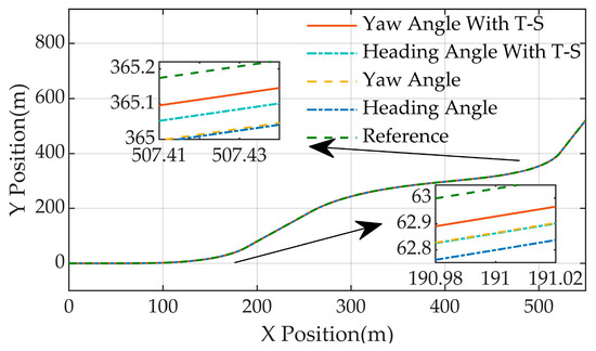
Figure 6.
The simulation results of path tracking on a serpentine road are compared.
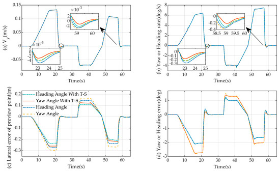
Figure 7.
The simulation results of the state vector on a serpentine road are compared. (a) Results of lateral velocity simulations are compared; (b) results of yaw velocity and heading velocity simulations are compared; (c) results of lateral deviation simulations are compared; (d) results of the yaw angle error and heading angle error simulations are compared.
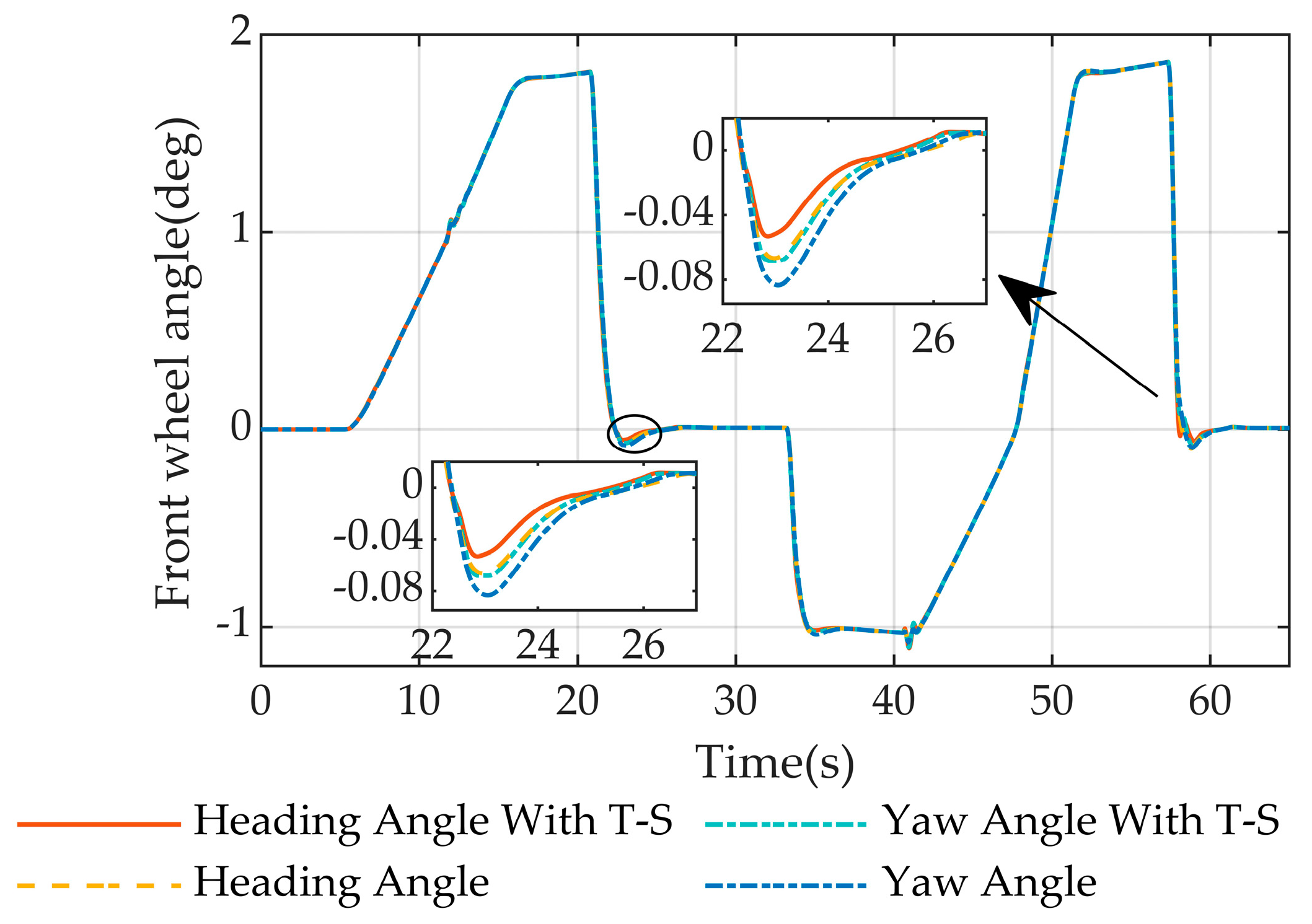
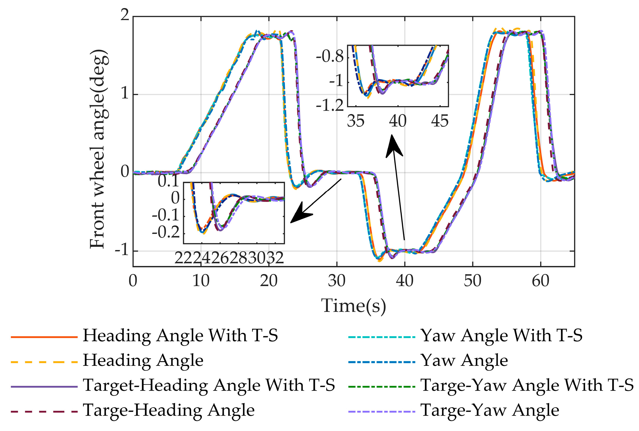
The comparative results of lateral velocity , yaw velocity and heading velocity , and front-wheel steering angle for the four model control algorithms are given in Figure 7a,b and Figure 8. As illustrated in the figure, the four model control algorithms have the same variation in the above three parameters when tracking a vehicle’s path. Figure 7d gives the results of the comparison of the yaw angle error and heading angle error . From the figure, it is evident that the magnitude of the yaw angle error is close to and does not exceed 2.8° for the two models, the yaw angle fuzzy model based on the yaw angle and the yaw angle model based on the yaw angle. The magnitude of the heading angle error of both models, the heading angle fuzzy-based model and heading angle-based model, is close to and does not exceed 2.1°. It is evident that the heading angle error is less than the yaw angle error .

Figure 8.
The simulation results of the front-wheel steering angle on a serpentine road are compared.
From the analysis of the above results, it is obtained that the algorithm for control based on the vehicle fuzzy model has a more excellent automatic trajectory performance. Comparing the algorithm for control based on the yaw angle fuzzy model with the algorithm for control based on the heading angle fuzzy model, the algorithm for control based on the heading angle fuzzy model has better automatic trajectory performance.
4.2. Double Lane Change Path Tracking
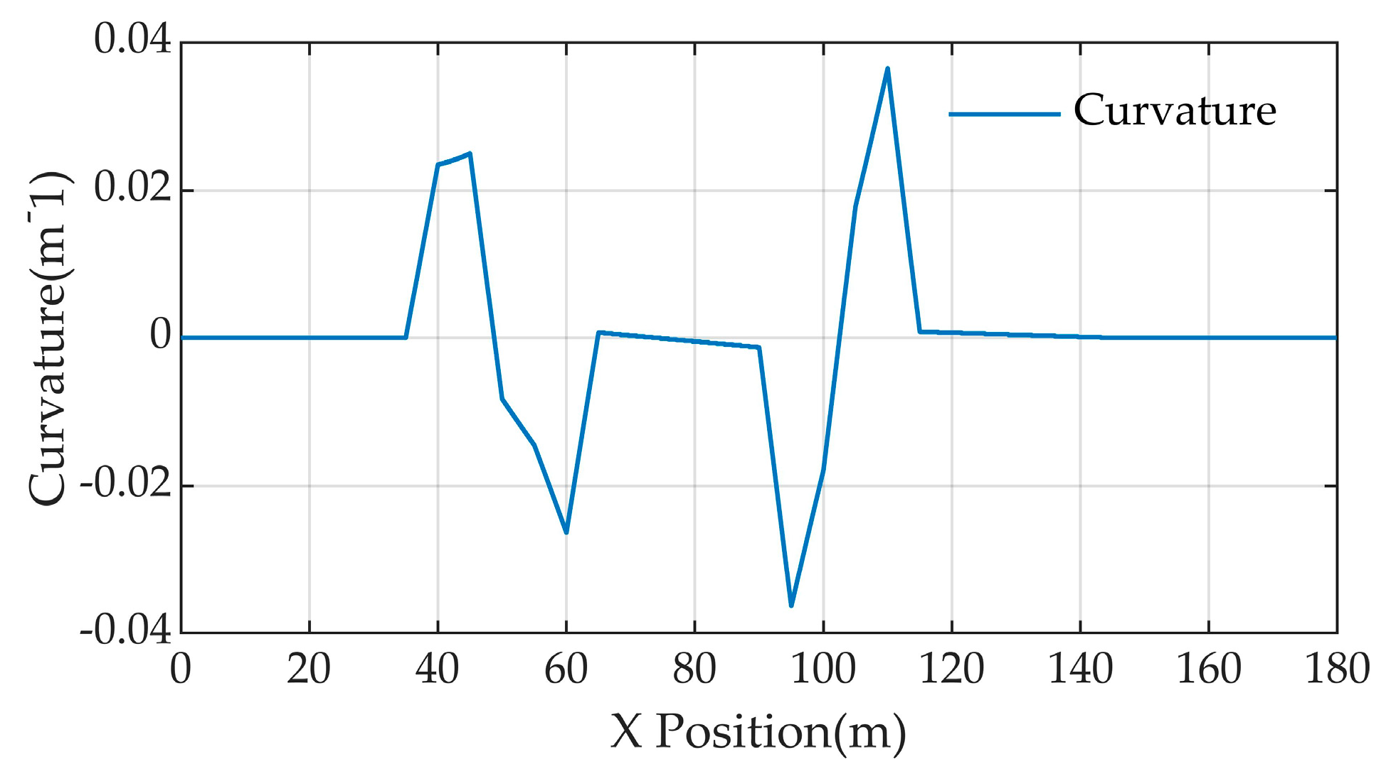
The speed variation of the autonomous vehicle for path tracking on a double lane change is shown in Figure 9; the speed is increased from the initial 30 km/h, after 10 s increments to 50 km/h, and after that the speed is uniform. The curvature of the double lane change changes, as shown in Figure 10, and the curvature changes in (−0.04, 0.04).
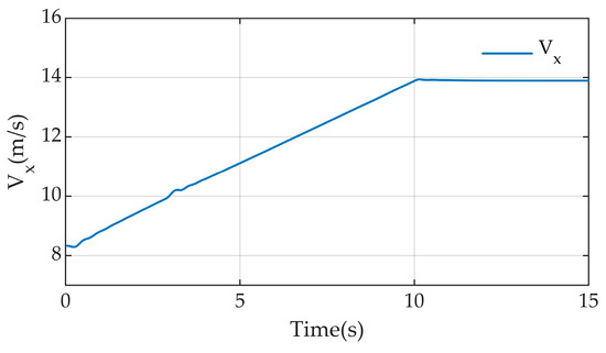
Figure 9.
Vehicle speed changes on a double lane change.
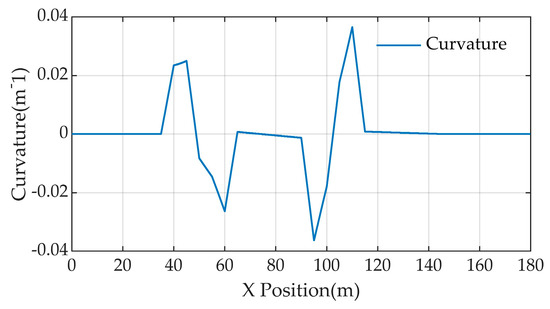
Figure 10.
Double lane change curvature.
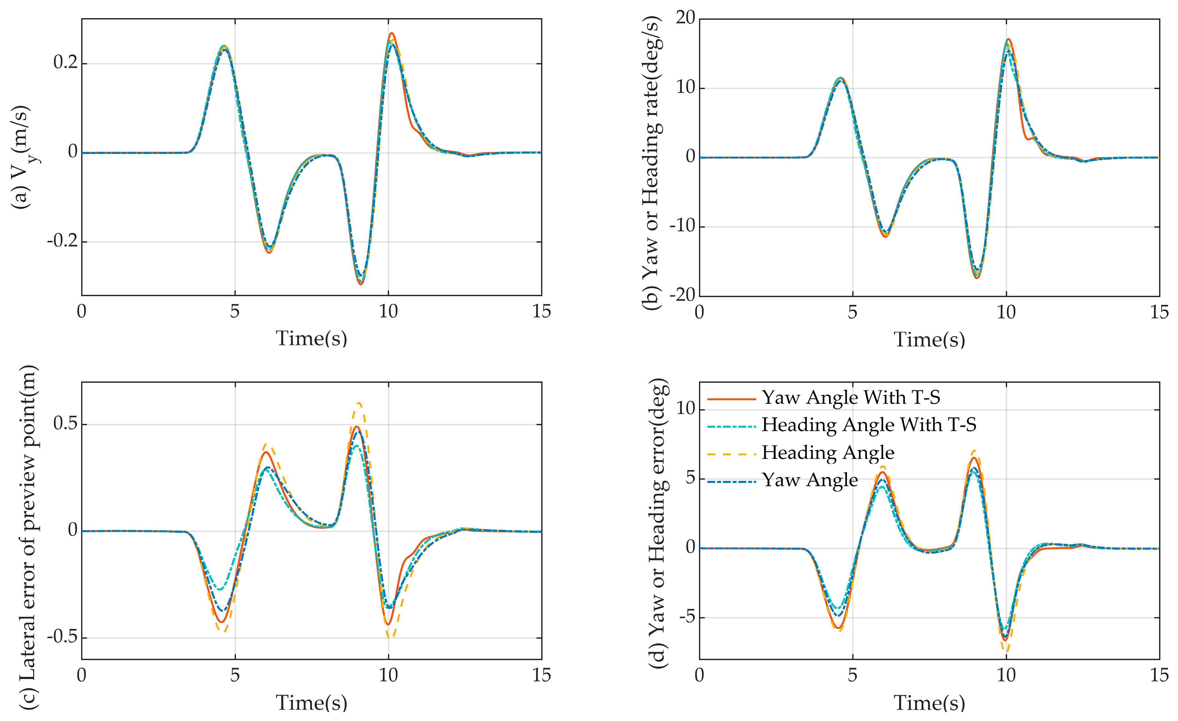
The path tracking and lateral deviation comparison results for the four model control algorithms are given in Figure 11 and Figure 12c. Based on the figure, it is evident that the maximum lateral deviation of the algorithm for control of the yaw angle model does not exceed 0.61 m, the maximum lateral deviation of the algorithm for control of the heading angle model does not exceed 0.51 m, the maximum lateral deviation of the algorithm for control based on the fuzzy model of the yaw angle does not exceed 0.47 m, the maximum lateral deviation of the algorithm for control based on the fuzzy model of the heading angle does not exceed 0.41 m, and the tracking accuracies of the paths of the four control algorithms are increased in order.
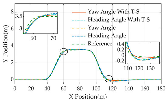
Figure 11.
The simulation results of path tracking on a double lane change are compared.
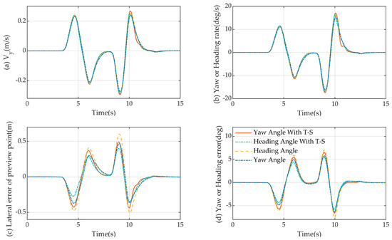
Figure 12.
The simulation results of the state vector on a double lane change are compared. (a) Results of lateral velocity simulations are compared; (b) results of yaw velocity and heading velocity simulations are compared; (c) results of lateral deviation simulations are compared; (d) results of the yaw angle error and heading angle error simulations are compared.
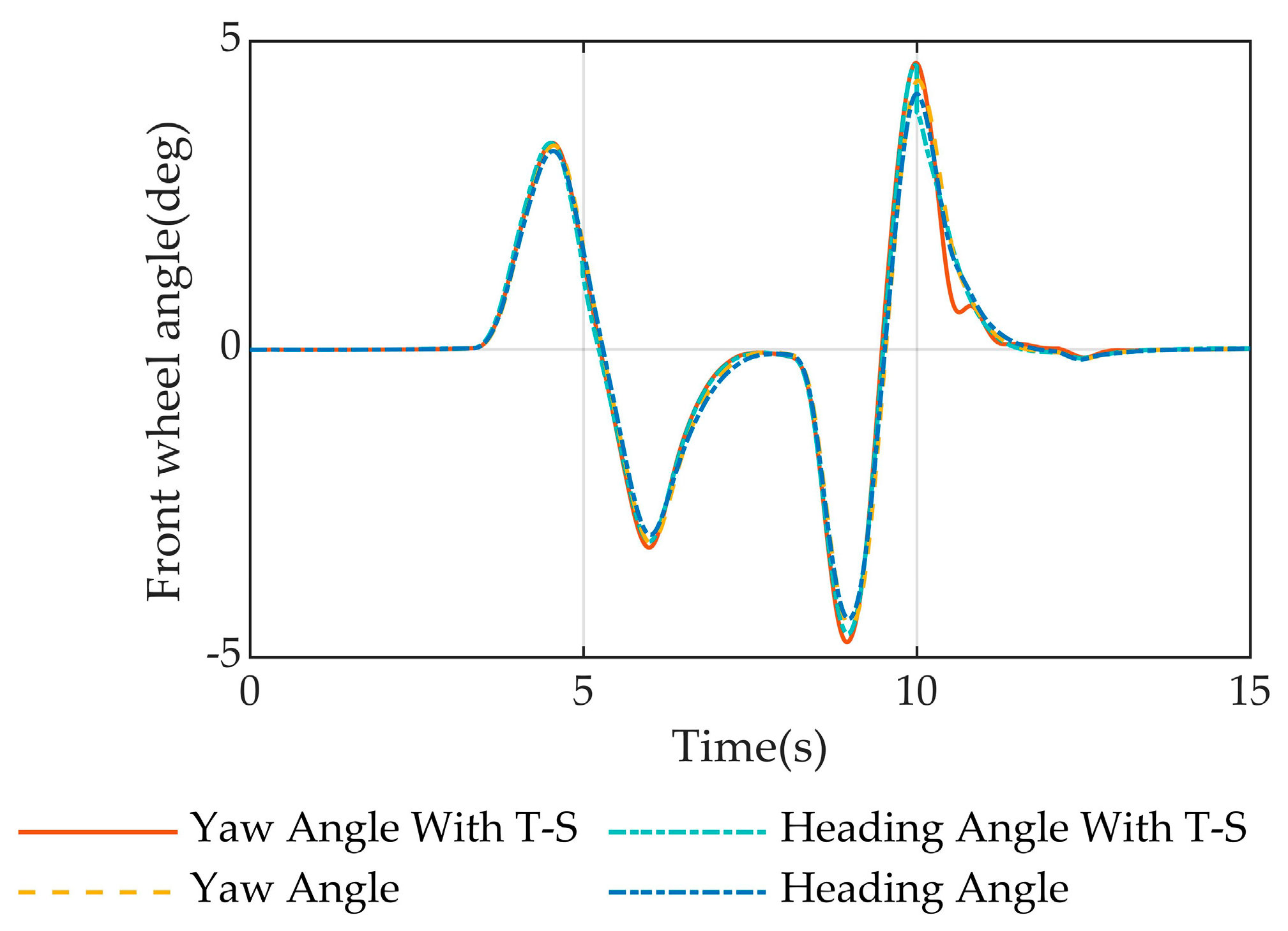
The comparative results of lateral velocity , yaw velocity and heading velocity , and front-wheel steering angle for the four model control algorithms are given in Figure 12a,b and Figure 13. As illustrated in the figure, the four model control algorithms have the same variation in the above three parameters when tracking a vehicle’s path. Figure 12d gives the results of the comparison of the yaw angle error and heading angle error . From the figure, it is evident that the magnitude of the yaw angle error is close to and does not exceed 7.3° for the two models, the yaw angle fuzzy model based on the yaw angle and the yaw angle model based on the yaw angle. The magnitude of the heading angle error of both models, the heading angle fuzzy-based model and heading angle-based model, is close to and does not exceed 6.2°. It is evident that the heading angle error is less than the yaw angle error .

Figure 13.
The simulation results of the front-wheel steering angle on a double lane change are compared.
By analyzing the above results in conjunction with the results of path tracking on serpentine roads by autonomous vehicles, it is demonstrated that the control algorithm based on the vehicle fuzzy model has more excellent automatic trajectory performance. Comparing the algorithm for control based on the yaw angle fuzzy model with the algorithm for control based on the heading angle fuzzy model, the algorithm for control based on the heading angle fuzzy model has better automatic trajectory performance.
5. Experimental Setup and Results
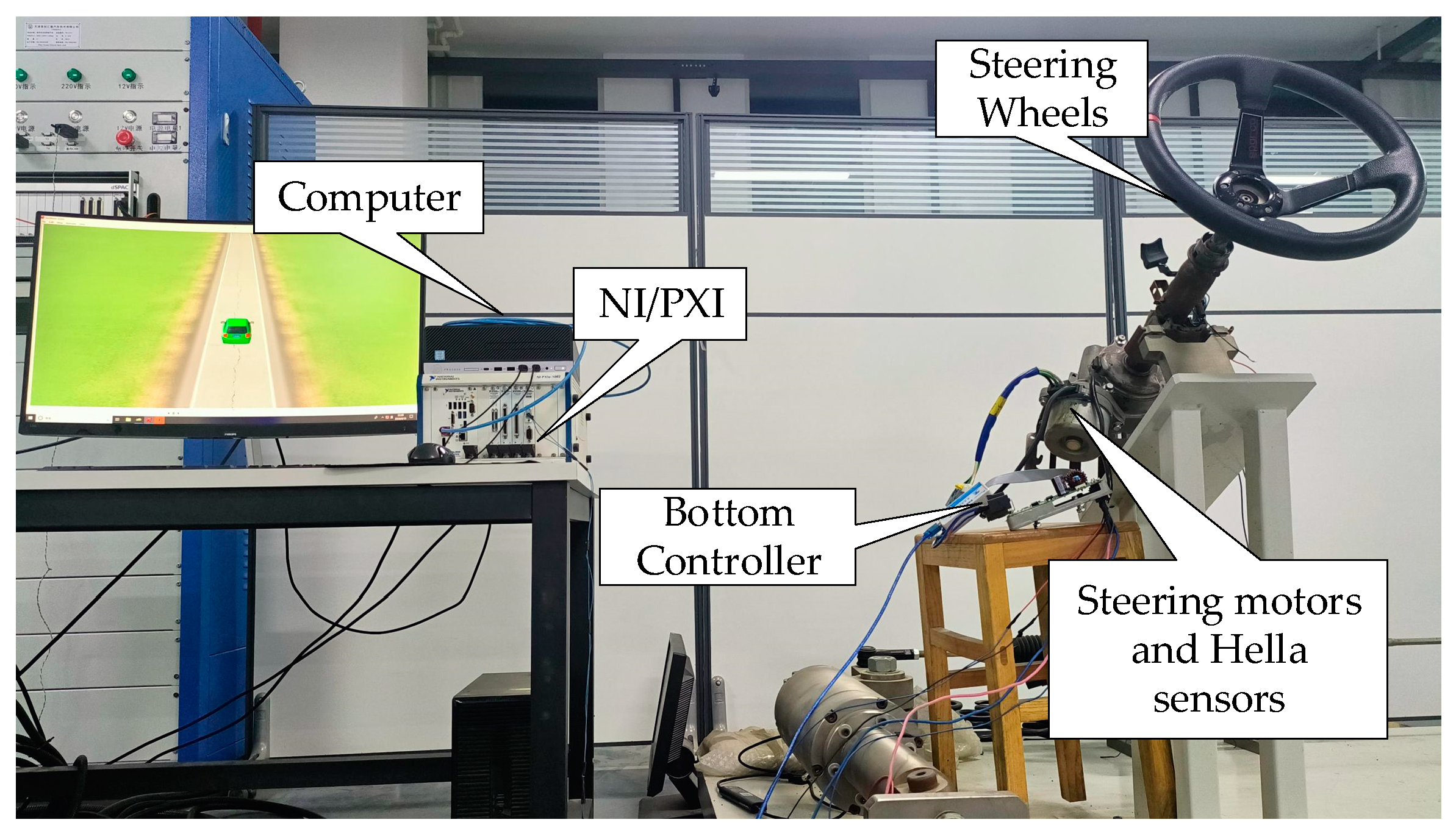
In this section, to validate the real-time performance of the two model control algorithms, hardware-in-the-loop (HIL) experiments are conducted using a serpentine road as an example in this paper. Figure 14 shows the structure of the control scheme based on the yaw or heading angle model. Figure 15 shows the steering control experimental bed used for the hardware-in-the-loop (HIL) experiments, and the related hardware includes the upper computer, the lower computer-NI/PXI system, and the steering system hardware.
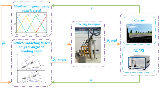
Figure 14.
Structure of the control scheme based on the model of the yaw angle or heading angle.
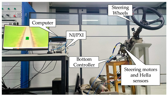
Figure 15.
Hardware-in-the-loop (HIL) test rig.
The upper computer controls the program via the LabView RT 2017 software. The lower computer-NI/PXI system is embedded in the real-time simulation scenario provided by CarSim (Ann Arbor, MI, USA), receives the actual steering angle transmitted by the steering system hardware, obtains the vehicle’s state quantities and other parameters in CarSim, obtains the target steering angle calculated by the algorithm of this paper through the above parameters, and finally sends the target steering angle to the steering system hardware. The steering system hardware includes items such as the steering wheel, sensors, and steering motor. One of the sensors used is the Hella sensor, which obtains information such as steering angle and steering. The steering motor receives the control signals sent by the bottom controller and controls them. The design of the bottom steering controller mainly relies on the 5744 chip, which is developed based on C language using the S32 environment. The bottom controller receives the target turning angle and sends the required control signals according to the target steering angle to drive the steering motor to rotate. All of the above hardware uses CAN for real-time information exchange.
To verify the conclusions obtained above, the four control algorithms mentioned above are experimented with path tracking at varying speeds, respectively.
Experiment-Path Tracking with Varying Vehicle Speed.
The path tracking and lateral deviation comparison results for the four model control algorithms are given in Figure 16 and Figure 17c. In the figure below the initial end of the arrow shows the position of the corresponding curve, and the end points to a magnified view at that position. Based on the figure, it is evident that the maximum lateral deviation of the algorithm for control of the yaw angle model does not exceed 0.57 m, the maximum lateral deviation of the algorithm for control of the heading angle model does not exceed 0.54 m, the maximum lateral deviation of the algorithm for control based on the fuzzy model of the yaw angle does not exceed 0.5 m, the maximum lateral deviation of the algorithm for control based on the fuzzy model of the heading angle does not exceed 0.47 m, and the tracking accuracies of the paths of the four control algorithms are increased in order.
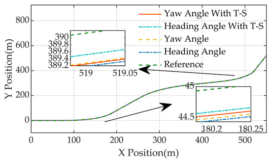
Figure 16.
The experimental results of path tracking on a serpentine road are compared.
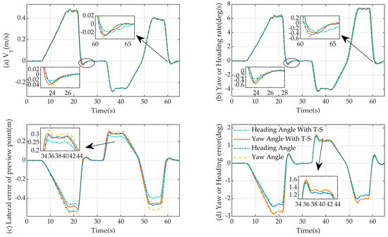
Figure 17.
The experimental results of the state vector on a serpentine road are compared. (a) Results of lateral velocity experimental are compared; (b) results of yaw velocity and heading velocity experimental are compared; (c), results of lateral deviation experimental are compared; (d) results of the yaw angle error and heading angle error experimental are compared.
Figure 17d gives the results of the comparison of the yaw angle error and heading angle error . From the figure, it is evident that the magnitude of the yaw angle error is close to and does not exceed 2.88° for the two models, the yaw angle fuzzy model based on the yaw angle and the yaw angle model based on the yaw angle. The magnitude of the heading angle error of both models, the heading angle fuzzy-based model and heading angle-based model, is close to and does not exceed 2.45°. It is evident that the heading angle error is less than the yaw angle error . The comparative results of lateral velocity , yaw velocity and heading velocity , and front-wheel steering angle for the four model control algorithms are given in Figure 17a,b, and Figure 18. As illustrated in the figure, the four model control algorithms have the same variation in the above three parameters when tracking a vehicle’s path.
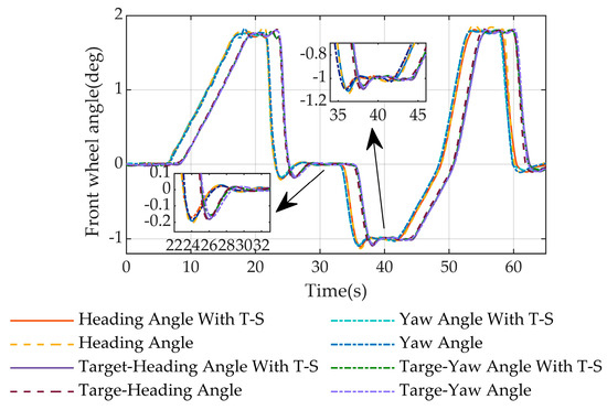
Figure 18.
The experimental results of front-wheel steering angle on a serpentine road are compared.
Where the target and actual front wheel steering angles for each of the four control methods are displayed in Figure 18, the graphic shows that the target steering angle’s size and the actual steering angle follow the same trend, and there exists only a lag of 1.5 s. The actual steering angle is the same as that of the target steering angle.
From the above hardware-in-the-loop (HIL) experimental results, the algorithm for control based on the vehicle fuzzy model has more excellent automatic trajectory performance. Comparing the algorithm for control based on the fuzzy model of yaw angle and the algorithm for control based on the fuzzy model of heading angle, the algorithm for control based on the fuzzy model of heading angle has better lateral stability and automatic trajectory performance.
Following analysis of the outcomes of hardware-in-the-loop (HIL) experiments and co-simulation using MATLAB 2021/Simulink–CarSim 8.02, the two results are similar, and both of them verified that the heading angle fuzzy model based on the fuzzy model has a more excellent automatic trajectory performance.
Since many parameters, such as vehicle or environment, vary over time, more time-varying parameters need to be selected to build the T-S fuzzy model in order to accurately portray the vehicle-road model, which increases the complexity of the control algorithm, thereby increasing the response time, etc., which further leads to an increase in the cost of the product. The accuracy of the control algorithm is inversely proportional to the product cost.
6. Conclusions
This work proposes a path-tracking control approach for autonomous cars based on the T-S fuzzy model of heading angle. First, the autonomous driving vehicle model based on heading angle is established by taking the intersection point between the vehicle traveling direction and the target path direction as the origin of the coordinate system and, in the significant side slip angle instances, the side slip angle is taken into consideration to enhance the precision of the vehicle’s road tracking. To guarantee that the control system can provide the best control law, the longitudinal speed of the vehicle is used as a variable parameter, and the domain and affiliation function is identified in order to build further a T-S fuzzy model based on heading angle. Inspired by the linear quadratic regulator (LQR) control, a performance metric function for heading angle state broadening error-based systems is defined to account for multiple control objectives. The system’s poles are limited to a fixed circular region to ensure a given dynamic performance. Ultimately, co-simulation with Matlab/Simulink–CarSim and hardware-in-the-loop (HIL) experiments are conducted. The outcomes demonstrate the superior automatic trajectory performance of the algorithm for control based on the fuzzy model of the vehicle with a heading angle. The advancement of automated driving control technology will be impacted by this study.
In future work, the introduction of observers into the model is considered to allow for the observation of parameters such as transverse velocity, which are difficult to measure. If the experimental conditions allow, real vehicle tests can be conducted to test the conditions under which the control algorithm is applicable.
Author Contributions
Conceptualization, J.W., Y.H. and X.L.; writing—original draft preparation, Y.H.; writing—review and editing, J.W., Y.H. and S.W.; methodology, J.W. and Y.H.; data curation, Y.H.; hardware, F.X., Y.H. and G.C.; software, Y.H., X.L. and G.C.; visualization, J.W.; formal analysis, F.X. and S.W. All authors have read and agreed to the published version of the manuscript.
Funding
This research was funded by the Shandong Province Key R and D Program (Major Science and Technology Innovation Project) Tasks, grant number 2023CXGC010214. This research also was funded by Shandong Province Key R and D Program (Competitive Innovation Platform), grant number 2022CXPT025.
Data Availability Statement
Data are contained within the article.
Conflicts of Interest
The authors declare no conflict of interest.
References
- Mahmud, K.; Gope, K.; Chowdhury, S.M.R. Possible causes & solutions of traffic jam and their impact on the economy of Dhaka City. J. Mgmt. Sustain. 2012, 2, 112. [Google Scholar]
- Gan, L. Globalization of the automobile industry in China: Dynamics and barriers in greening of the road transportation. Energy Policy 2003, 31, 537–551. [Google Scholar] [CrossRef]
- Yuan, X.; Liu, H.; Qi, R. Research on key technologies of autonomous driving platform. J. Phys. Conf. Ser. 2021, 1754, 012127. [Google Scholar] [CrossRef]
- Narla, S.R. The evolution of connected vehicle technology: From smart drivers to smart cars to… self-driving cars. Ite J. 2013, 83, 22–26. [Google Scholar]
- Sorniotti, A.; Barber, P.; De Pinto, S. Path tracking for automated driving: A tutorial on control system formulations and ongoing research. In Automated Driving: Safer and More Efficient Future Driving; Springer: Cham, Switzerland, 2017; pp. 71–140. [Google Scholar]
- Wang, R.; Ye, Q.; Cai, Y.; Wang, Y.; Xu, X.; Meng, X.; Long, C. Analyzing the influence of automatic steering system on the trajectory tracking accuracy of intelligent vehicle. Adv. Eng. Softw. 2018, 121, 188–196. [Google Scholar] [CrossRef]
- Wu, H.; Li, Z.; Si, Z. Trajectory tracking control for four-wheel independent drive intelligent vehicle based on model predictive control and sliding mode control. Adv. Mech. Eng. 2021, 13, 16878140211045142. [Google Scholar] [CrossRef]
- Li, X.; Chan, C.-Y.; Wang, Y. A reliable fusion methodology for simultaneous estimation of vehicle sideslip and yaw angles. IEEE Trans. Veh. Technol. 2015, 65, 4440–4458. [Google Scholar] [CrossRef]
- Yang, M.; Chen, C.-F.; Shu, M.-L.; Yang, Y.-Y. Path Tracking Control for Uncertainty Vehicles via LMI Optimization. In Proceedings of the 3rd International Conference on Wireless Communication and Sensor Networks (WCSN 2016), Wuhan, China, 10–11 December 2016; pp. 338–344. [Google Scholar]
- Hang, P.; Chen, X.; Luo, F.; Fang, S. Robust control of a four-wheel-independent-steering electric vehicle for path tracking. SAE Int. J. Veh. Dyn. Stab. NVH 2017, 1, 307–316. [Google Scholar] [CrossRef]
- Yang, Z.; Huang, J.; Yang, D.; Zhong, Z. Design and optimization of robust path tracking control for autonomous vehicles with fuzzy uncertainty. IEEE Trans. Fuzzy Syst. 2021, 30, 1788–1800. [Google Scholar] [CrossRef]
- Chen, M.; Ren, Y.; Ou, M. Adaptive robust path tracking control for autonomous vehicles considering multi-dimensional system uncertainty. World Electr. Veh. J. 2023, 14, 11. [Google Scholar] [CrossRef]
- Shen, H.; Ling, R.; Mao, J.; Li, S. Steering control strategy guide by two preview vision cues. Sci. China Technol. Sci. 2012, 55, 2662–2670. [Google Scholar] [CrossRef]
- Hiraoka, T.; Nishihara, O.; Kumamoto, H. Automatic path-tracking controller of a four-wheel steering vehicle. Veh. Syst. Dyn. 2009, 47, 1205–1227. [Google Scholar] [CrossRef]
- Hang, P.; Chen, X. Path tracking control of 4-wheel-steering autonomous ground vehicles based on linear parameter-varying system with experimental verification. Proc. Inst. Mech. Eng. Part I J. Syst. Control. Eng. 2021, 235, 411–423. [Google Scholar] [CrossRef]
- Jin, X.J.; Yin, G.; Chen, N. Gain-scheduled robust control for lateral stability of four-wheel-independent-drive electric vehicles via linear parameter-varying technique. Mechatronics 2015, 30, 286–296. [Google Scholar] [CrossRef]
- Hu, H.; Bei, S.; Zhao, Q.; Han, X.; Zhou, D.; Zhou, X.; Li, B. Research on trajectory tracking of sliding mode control based on adaptive preview time. Actuators 2022, 11, 34. [Google Scholar] [CrossRef]
- Mokhtare, Z.; Vu, M.; Mobayen, S.; Fekih, A. Design of an LMI-Based Fuzzy Fast Terminal Sliding Mode Control Approach for Uncertain MIMO Systems. Mathematics 2022, 10, 1236. [Google Scholar] [CrossRef]
- Chatavi, M.; Vu, M.T.; Mobayen, S.; Fekih, A. H∞ robust LMI-based nonlinear state feedback controller of uncertain nonlinear systems with external disturbances. Mathematics 2022, 10, 3518. [Google Scholar] [CrossRef]
- Sheikhsamad, M.; Puig, V. Learning-Based Control of Autonomous Vehicles Using an Adaptive Neuro-Fuzzy Inference System and the Linear Matrix Inequality Approach. Sensors 2024, 24, 2551. [Google Scholar] [CrossRef] [PubMed]
- Chen, C.; Jia, Y.; Shu, M.; Wang, Y. Hierarchical adaptive path-tracking control for autonomous vehicles. IEEE Trans. Intell. Transp. Syst. 2015, 16, 2900–2912. [Google Scholar] [CrossRef]
- Du, H.; Zhang, N.; Naghdy, F. Velocity-dependent robust control for improving vehicle lateral dynamics. Transp. Res. Part C Emerg. Technol. 2011, 19, 454–468. [Google Scholar] [CrossRef]
- Feng, J.; Yin, G.; Liang, J.; Lu, Y.; Xu, L.; Zhou, C.; Peng, P.; Cai, G. A Robust Cooperative Game Theory based Human-machine Shared Steering Control Framework. IEEE Trans. Transp. Electrif. 2023; Early Access. [Google Scholar] [CrossRef]
- Liang, J.; Wang, F.; Feng, J.; Zhao, M.; Fang, R.; Pi, D.; Yin, G. A Hierarchical Control of Independently Driven Electric Vehicles Considering Handling Stability and Energy Conservation. IEEE Trans. Intell. Veh. 2023, 9, 38–751. [Google Scholar] [CrossRef]
- He, X.; Huang, W.; Lv, C. Trustworthy autonomous driving via defense-aware robust reinforcement learning against worst-case observational perturbations. Transp. Res. Part C Emerg. Technol. 2024, 163, 104632. [Google Scholar] [CrossRef]
- He, X.; Liu, Y.; Yang, K.; Wu, J.; Ji, X. Robust coordination control of AFS and ARS for autonomous vehicle path tracking and stability. In Proceedings of the 2018 IEEE International Conference on Mechatronics and Automation (ICMA), Changchun, China, 5–8 August 2018; pp. 924–929. [Google Scholar]
- Wu, J.; Kong, Q.; Yang, K.; Liu, Y.; Cao, D.; Li, Z. Research on the steering torque control for intelligent vehicles co-driving with the penalty factor of human–machine intervention. IEEE Trans. Syst. Man Cybern. Syst. 2022, 53, 59–70. [Google Scholar] [CrossRef]
- He, X.; Lou, B.; Yang, H.; Lv, C. Robust decision making for autonomous vehicles at highway on-ramps: A constrained adversarial reinforcement learning approach. IEEE Trans. Intell. Transp. Syst. 2022, 24, 4103–4113. [Google Scholar] [CrossRef]
- Wu, J.; Zhang, J.; Nie, B.; Liu, Y.; He, X. Adaptive control of PMSM servo system for steering-by-wire system with disturbances observation. IEEE Trans. Transp. Electrif. 2021, 8, 2015–2028. [Google Scholar] [CrossRef]
- Tseng, C.-S.; Chen, B.-S.; Uang, H.-J. Fuzzy tracking control design for nonlinear dynamic systems via TS fuzzy model. IEEE Trans. Fuzzy Syst. 2001, 9, 381–392. [Google Scholar] [CrossRef]
- He, X.; Wu, J.; Huang, Z.; Hu, Z.; Wang, J.; Sangiovanni-Vincentelli, A.; Lv, C. Fear-neuro-inspired reinforcement learning for safe autonomous driving. IEEE Trans. Pattern Anal. Mach. Intell. 2023, 46, 267–279. [Google Scholar] [CrossRef] [PubMed]
- He, X.; Huang, W.; Lv, C. Toward Trustworthy Decision-Making for Autonomous Vehicles: A Robust Reinforcement Learning Approach with Safety Guarantees. Engineering 2024, 33, 77–89. [Google Scholar] [CrossRef]
- Wang, C.; Qin, J.; Guo, M.; Xu, Y. Prediction of vehicle trajectory based on Fuzzy colored petri net. TELKOMNIKA Indones. J. Electr. Eng. 2013, 11, 5824–5832. [Google Scholar] [CrossRef]
- He, X.; Yang, H.; Hu, Z.; Lv, C. Robust lane change decision making for autonomous vehicles: An observation adversarial reinforcement learning approach. IEEE Trans. Intell. Veh. 2022, 8, 184–193. [Google Scholar] [CrossRef]
- Wang, J.; Zhang, G.; Wang, R.; Schnelle, S.C.; Wang, J. A gain-scheduling driver assistance trajectory-following algorithm considering different driver steering characteristics. IEEE Trans. Intell. Transp. Syst. 2016, 18, 1097–1108. [Google Scholar] [CrossRef]
- Xie, W. An equivalent LMI representation of bounded real lemma for continuous-time systems. J. Inequalities Appl. 2008, 2008, 1–8. [Google Scholar] [CrossRef]
- Liang, J.; Feng, J.; Fang, Z.; Lu, Y.; Yin, G.; Mao, X.; Wu, J.; Wang, F. An energy-oriented torque-vector control framework for distributed drive electric vehicles. IEEE Trans. Transp. Electrif. 2023, 9, 4014–4031. [Google Scholar] [CrossRef]
- Lee, H.J.; Park, J.B.; Chen, G. Robust fuzzy control of nonlinear systems with parametric uncertainties. IEEE Trans. Fuzzy Syst. 2001, 9, 369–379. [Google Scholar]
- Liang, J.; Tian, Q.; Feng, J.; Pi, D.; Yin, G. A polytopic model-based robust predictive control scheme for path tracking of autonomous vehicles. IEEE Trans. Intell. Veh. 2023, 9, 3928–3939. [Google Scholar] [CrossRef]
- Benloucif, A.; Nguyen, A.-T.; Sentouh, C.; Popieul, J.-C. Cooperative trajectory planning for haptic shared control between driver and automation in highway driving. IEEE Trans. Ind. Electron. 2019, 66, 9846–9857. [Google Scholar] [CrossRef]
- Zhang, H.; Zhang, X.; Wang, J. Robust gain-scheduling energy-to-peak control of vehicle lateral dynamics stabilisation. Veh. Syst. Dyn. 2014, 52, 309–340. [Google Scholar] [CrossRef]
- Taheri, S.; Rakheja, S.; Hong, H. Influence of human driving characteristics on path tracking performance of vehicle. In Proceedings of the Intelligent Robotics and Applications: 5th International Conference, ICIRA 2012, Montreal, QC, Canada, 3–5 October 2012; Proceedings, Part II 5, 2012. pp. 207–216. [Google Scholar]
Disclaimer/Publisher’s Note: The statements, opinions and data contained in all publications are solely those of the individual author(s) and contributor(s) and not of MDPI and/or the editor(s). MDPI and/or the editor(s) disclaim responsibility for any injury to people or property resulting from any ideas, methods, instructions or products referred to in the content. |
© 2024 by the authors. Licensee MDPI, Basel, Switzerland. This article is an open access article distributed under the terms and conditions of the Creative Commons Attribution (CC BY) license (https://creativecommons.org/licenses/by/4.0/).

