Abstract
The expansion of DC electrical distribution systems necessitates advancements in detecting and mitigating DC arc events, a significant contributor to fire accidents in low-voltage DC distribution systems. Detecting DC arc faults poses considerable challenges, making them a major safety concern in DC power lines. Conventional approaches mainly rely on arc current, which can vary during normal operation, potentially leading to false alarms. Moreover, these methods often require manual adjustment of detection thresholds for different systems, introducing the risk of malfunction. This study proposes an advanced arc fault recognition procedure that extracts and utilizes various key features for the DC arc detection. This work investigated new various features, which are the square average, the average, the median, the rms, the peak-to-peak, and the variance values, to find out which one can be the most effective features to detect the DC arc failure. The results of this detection process show good evidence for the effectiveness and reliability of the proposed malfunction detecting plan.
1. Introduction
Despite the myriad advantages that DC systems offer over AC systems, their extensive implementation has been impeded by the absence of fully developed and stable transmission and distribution tools. Safety is a paramount concern for practical DC system implementation [1,2,3]. DC arc faults, often overlooked by fault protection equipment, pose severe fire hazards in DC power systems [4]. Unlike AC systems, DC systems lack a current zero point, making them susceptible to the development and sustained presence of high-temperature plasma arc discharges during electric arc faults, which can lead to disastrous electric fires [5,6]. Additionally, if a DC arc persists, it can escalate into a large-scale fire hazard [7]. Detecting and interrupting series arc faults before they escalate is crucial. Arc faults are accompanied by distinctive characteristics, including sound, light, heat rises, distortion voltage, and high-frequency component signals [8]. Previous research has focused on modeling DC arc faults, both theoretically and experimentally [9,10,11]. Two types of arc faults are possible: parallel and series. Parallel arc faults are usually caused by short circuits and are relatively easier to detect. However, series arc faults, occurring in conductors carrying normal load currents, are more challenging to detect and locate [12]. The voltage and current characteristics of arc faults have been extensively studied in both time and frequency domains [13,14,15]. Detection methods based solely on time domain information require careful threshold selection to avoid false alarms. Series arc faults typically introduce high-frequency components into the circuit current [16,17]. Machine learning algorithms have shown promise in DC arc fault detection. Nevertheless, current methodologies frequently concentrate exclusively on time or frequency domain currents, overlooking the necessity for inclusive preprocessing of signals [18,19,20,21,22,23,24,25,26,27,28], although an approach with simple indexes has been tried for DC arc detection [19].
This research presents a novel methodology to detect arc fault recognition by extracting and utilizing various key features for DC arc detection. This work investigated new features, namely the square average, the average, the median, the rms, the peak-to-peak, and the variance values, to find out which one can be the most effective features to detect DC arc failure using intelligent learning models (ILMs) to tackle the complex issue of DC arc fault diagnosis. The diagnostic outcomes validate the remarkable effectiveness of this approach in improving detecting results. This paper is outlined as follows: Section 2 comprehensively details the configuration of the arc setup, explicating the alterations in current characteristics throughout different domains during different phases, as well as an in-depth discussion of the ILMs utilized for arc fault detection. Section 3 reports the deductions of the fault diagnosis techniques with various features, covering scenarios involving different current scales and functioning rates. Lastly, Section 3 synthesizes the cumulative discoveries and comprehensions obtained from the application of ILMs in arc fault detection, culminating in the conclusion of this study.
2. Hardware Specifications and Data Processing
2.1. Hardware Specifications
In order to emulate intentional DC arc faults in DC power lines connected with very popular three-phase switching loads in practical DC power systems, the arc generator was installed between the three-phase voltage source inverter and the DC power source. The three-phase voltage source inverter was used to generate three-phase balanced adjustable sinusoidal ac voltages and currents. Different switching frequencies and different output current magnitudes were produced by the three-phase voltage source inverters, to test effectiveness of the developed algorithm under a variety of operating conditions for the three-phase voltage source inverter. The three-phase voltage source inverter was controlled by a common space vector pulse-width modulation technique, which can synthesize the variable magnitude and variable frequencies of three-phase AC output voltage waveforms. The space vector pulse-width modulation method was programmed in a digital signal processor to control the three-phase voltage source inverter. Figure 1 provides a hardware setup for acquiring DC arc data based on the standard in UL1699B [23]. The recorded data underwent a careful investigation with MATLAB software. The setup involved fundamental modules, including a power supply, failure generator, and load parts. Of particular significance was the N8741A DC source, generously provided by Keysight Technologies, USA, and which prominently features in Figure 1. This power source supply provided a power range of 0–100 V and a current range of 0–20 A, with voltage and current resolutions of 1 mV and 1 mA, respectively. The precision of the arc rod separation was impeccably executed through the highly accurate activation of a step motor intricately linked with these rods. On the other hand, the authors harnessed the abilities of an oscilloscope working at a sampling rate of 250 kHz. The oscilloscope used was the Tektronix MSO3054 (Beaverton, OR, USA) boasting a bandwidth of 500 MHz, four analog channels, and a sample rate of 5 GS/s per channel. The current possession procedure was additionally assisted by the Tektronix TCP312 current probe, guaranteeing the exact measurement of arc currents. The Tektronix TCP312 current probe, featuring a bandwidth of DC to 100 MHz and a maximum input current of 30 A continuous (50 A peak), offered sensitivity ranging from 10 mA/div to 50 A/div. Our comprehensive investigation of DC arc failure spanned different domains. Systematic initiation of DC arcs took place under a varied range of investigational conditions. The investigational factors were thoroughly specified, using a DC source of 300 V. The authors investigated a variety of current scales of 5 and 8 A, within different switching rates. The experiments were performed using the load combinations of resistor (10 Ω) and inductor (10 mH). Furthermore, Figure 1 offers a visual representation of the fundamental configuration of the three-phase DC-AC converters, which were pivotal as the main load modules in our investigation and constructed from the insulated gate bipolar transistor (IGBT). Additionally, the IGBT module (SKM50GB123D, SEMIKRON, Nuremberg, Germany) boasted a maximum collector current of 100 A and a maximum collector–emitter voltage of 1200 V, with an operating temperature range of −40 °C to 125 °C. The inverters were qualified to convert DC–AC signals. Throughout our research, we maintained precise control over these inverter units by implementing space vector modulation (SVPWM)., The SVPWM method was realized in a Texas Instrument (TI) digital signal processor (DSP) to synthesize the well-regulated balanced three-phase sinusoidal output currents in three-phase ac loads. The main aim was to employ a predestined DC voltage while operating the on and off conditions of the six switches, thereby emulating the sinusoidal signals that characterize the AC network. This high level of control enabled us to make meticulous adjustments to both the rate and amplitude parameters, confirming the accurate and reliable adjustment of our experiments.

Figure 1.
Arc hardware setup. (a) Experimental circuit. (b) Arc generator. (c) Arcing event.
2.2. Failure Event Descriptions
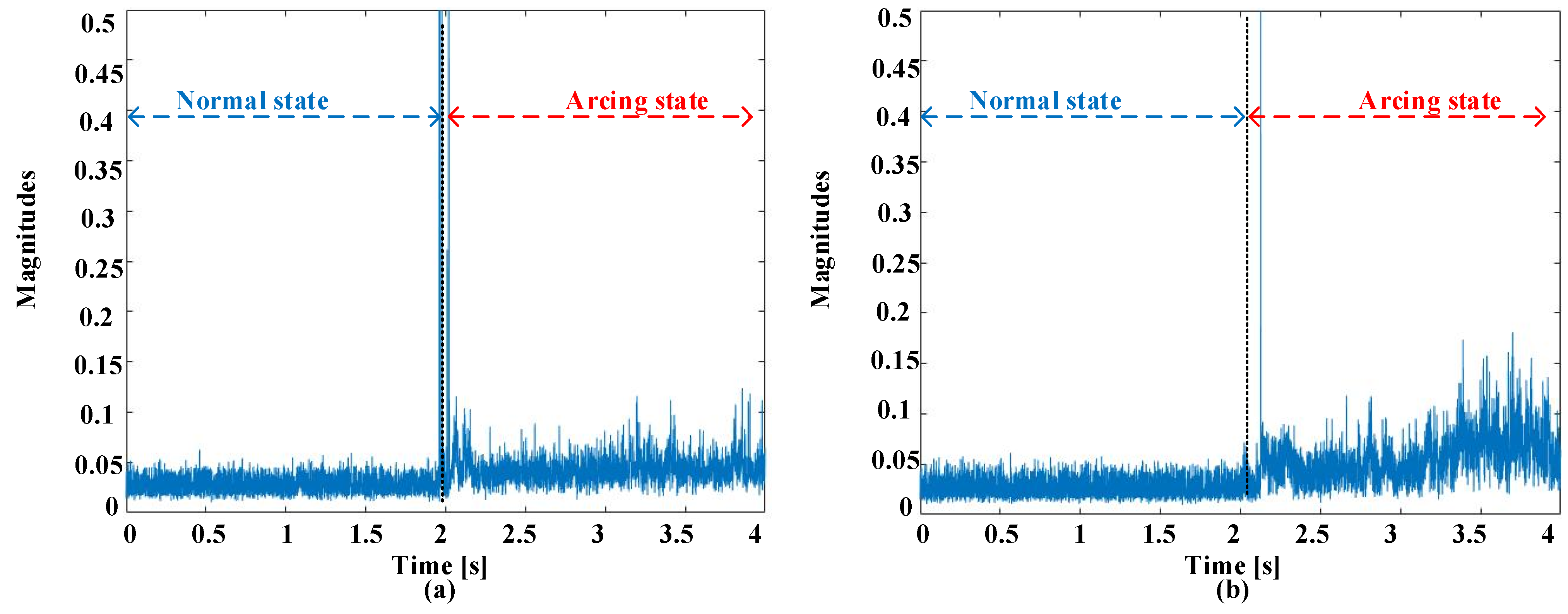
Figure 2 offers a visual representation elucidating the waveforms observed in the time domains, showcasing instances of ordinary working and the inception of failure experiences at switching frequencies of 5 kHz. These observations encompass two scenarios, one with a current amplitude of 5 A and another with an amplitude of 8 A. Prior to the initiation of arcing, there is a discernible uniformity in waveform characteristics across various current amplitudes and switching frequencies. Nonetheless, the establishment of an electric failure into the circuit injects a myriad of abnormalities into these signals. These anomalies entail an increased prevalence of harmonic components overlaid on the load current, a deformation leading to distorting characteristics, and a slight reduction in the amount of the existing current. The initial phase of the failure incident is conspicuously characterized by prominent spikes in amplitude. These spikes are a straightforward effect of the heated leak of electrical flashes. It is imperative to underscore that the exposed and uncharacteristic occurrences sustain meaningful promise as distinctive pointers within the realm of arc fault detection. Indeed, the behavior of the current during arcing events can exhibit variations that may not align with conventional expectations. In this study, the authors have observed that while there is a general trend of current reduction during the onset of arcing, there are also instances where large fluctuations occur at the beginning of the fault event. These fluctuations are often characterized by sudden spikes in amplitude and may not follow a regular cycling pattern. These abrupt fluctuations in current amplitude can be attributed to the dynamic nature of arc discharge. When an electrical arc is initiated, there is a rapid and chaotic exchange of energy between the electrodes, resulting in the formation of fiery sparks and the generation of high-frequency harmonics. These transient phenomena manifest as sharp peaks in the current waveform, indicating the presence of arcing activity. It is important to note that the behavior of the current during arcing events can vary depending on other factors, such as the severity of the fault, the characteristics of the arc, and the surrounding circuit conditions. While a reduction in current may be observed as the fault progresses, the initial stages of the arcing event are often characterized by these erratic fluctuations and transient spikes in amplitude. Therefore, in Figure 2, the observed reduction in current during arcing is accompanied by the presence of conspicuous spikes and abnormalities in the waveform, highlighting the complex nature of arc fault phenomena.
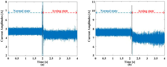
Figure 2.
Waveforms at the rate of 5 kHz in time domains. (a) 5 A current amplitude. (b) 8 A current amplitude.
Conversely, a completely distinct pattern materializes following the initiation of the arc event. This pattern is marked by the noticeable emergence of a multitude of distortions prominently evident inside the spectrum covering a specified range (3–30 kHz). These complex interactions within the frequency spectrum provide valuable insights into the distinctive characteristics of both switching noise and arc-induced distortions, enhancing our understanding of the underlying phenomena.
2.3. Screening Procedures in Time and Frequency Domains
Table 1 presents the structural parameters of the various learning models utilized in this study. A support vector machine (SVM) is a powerful tool for effective classification tasks, as it identifies the optimal hyperplane that maximizes the margin between different groups, aiding in the separation of data points into multiple categories. This hyperplane acts as the decision boundary, effectively distinguishing between diverse groups of data points. SVMs find application in various fields, such as text classification, image classification, face detection, bioinformatics, and financial modeling due to its versatility. When using SVM, it is essential to select appropriate values for certain parameters, like gamma and C, to prevent overfitting or underfitting. The value of C should be chosen optimally, as it regulates the trade-off between a smooth decision boundary and correct classification. Similarly, the gamma value determines the curvature of the decision boundary, with higher values resulting in more curvature and lower values leading to less curvature. In this context, a regulation parameter C of 1, a radial basis function kernel function, degree 3, and an automatic gamma value are commonly used settings [24]. K-nearest neighbor (KNN) is a classification algorithm that assigns a class label to an input data point based on the majority class among its k-nearest neighbors. It calculates the distances between each data point and others in the data set, typically using the Euclidean distance metric. The algorithm then selects the k-nearest data points with the smallest distances as neighbors. In this context, a common choice for the number of neighbors (k) is 20. KNN operates using a brute force algorithm type, where distances are computed for all pairs of points in the data set. This approach ensures that the nearest neighbors are accurately identified and considered in the classification process [25]. Decision trees (DTs) are versatile algorithms that recursively split data into subsets based on significant features to maximize information gain. This process continues until a stopping criterion is met, resulting in a tree structure that represents decision rules for partitioning data into classes or making predictions. Decision nodes within the tree represent decisions based on feature values, with branches for possible outcomes, while leaf nodes correspond to final predictions. In this case, the decision tree type used is the classification and regression tree (CART), suitable for both classification and regression tasks. The depth of the tree, which determines the maximum number of splits, is set to 4 with 14 leaf nodes [26]. Ensemble learning, a powerful technique in machine learning, combines predictions from multiple models to enhance accuracy and reliability. Random forest (RF) is a popular ensemble method that creates an ensemble of decision trees. The forest size, which can vary from 100 to 1000 trees, allows for a balance between performance and computational resources. RF overcomes the limitations of individual decision trees by implementing bootstrap aggregation, where each tree is trained on a random subset of the data and considers a random subset of features. In this case, the RF consists of 500 decision trees, ensuring robustness and diversity in the ensemble [27]. Naive Bayes (NB) is a probabilistic classifier widely used for classification tasks. It calculates the probability of a data point belonging to different classes and assigns the class with the highest probability as the predicted class. NB employs Bayes’ theorem to compute class probabilities based on the features associated with the data point. Despite its “naive” assumption of feature independence, NB remains effective due to its simplicity and efficiency. In this case, the naive Bayes classifier adopts a Gaussian distribution model, with hyperparameter optimization performed using a Bayesian approach. This model assumes a normal distribution of features, allowing it to effectively classify data points based on their probabilities [28].

Table 1.
Specifications of learning models.
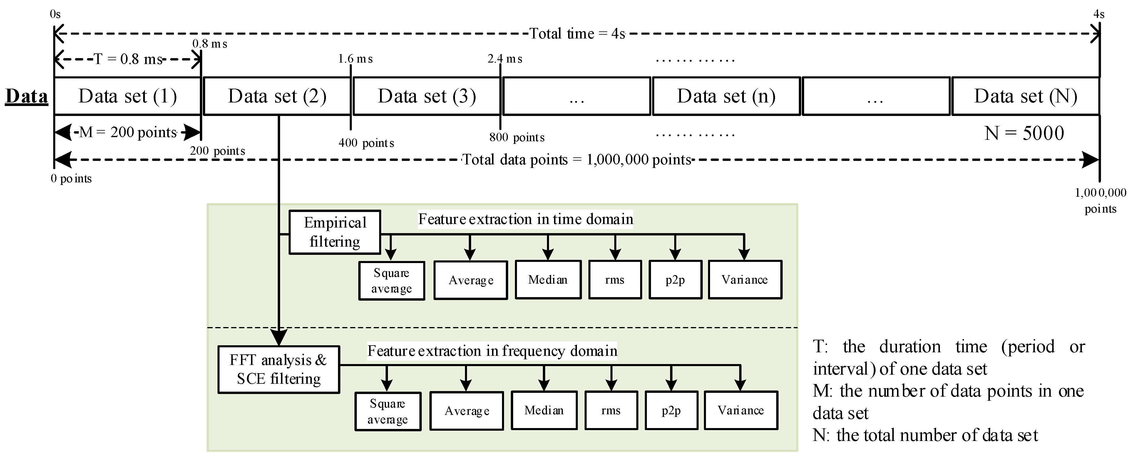
The empirical rule, also known as the 68–95–99.7 rule or the three-sigma rule, represents a foundational rule in statistics. It posits that in the data conforming to a normal distribution, an overwhelmingly significant greater part, roughly 99.7%, of experiential statistics elements are concentrated inside the range of the three standard deviations (±3sig) aligned nearby the mean (mu) [24]. To elaborate, it predicts that approximately 95% of data are located inside the space of the two standard deviations (mu ± 2sig), while roughly 68% exist in the span of the one standard deviation (mu ± sig). Figure 3 presents the process of feature extraction in this study. The data, sampled at a rate of 250 kHz, is partitioned into separated portions, each with a period or interval (T) of 0.8 ms, to assist the filtering procedure. Inside these individual segments or data sets, each segment contains 200 data points, and the standard deviation and the mean are computed.
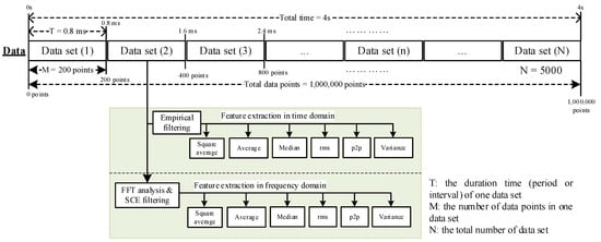
Figure 3.
Feature extraction process.
We establish three distinct empirical filtering ranges for each data set, and after filtering, the features of each data set are obtained as follows:
where is the data point at position in the data set ( varies from 1 to 200), M is the number of data points in an every period, M is equal to 200 in this study, and data set(n) denotes the particular data set sampled at specific moment (n varies from 1 to 5000). The equations outlined in this paper function as statistical tools applied to each data set, extracting specific characteristics crucial for analyzing arc faults. These equations, including metrics, like averages, medians, root mean square (RMS) values, peak-to-peak amplitudes, variances, and other pertinent parameters, are individually employed on each data set. Each data set represents a unique moment or time interval during which electrical signals were sampled and logged. In contrast, the figures in this paper depict the amalgamation of these features across all data sets, with each data set encapsulating a time interval of 0.8 milliseconds. These figures offer a holistic perspective on the arc fault behavior over time. The curves in the figures represent a collective view of features extracted from multiple data sets, each corresponding to a specific moment in time. By aggregating feature values from all data sets, the overall trend or pattern in arc fault behavior is captured, facilitating a comprehensive understanding of its dynamics and characteristics.
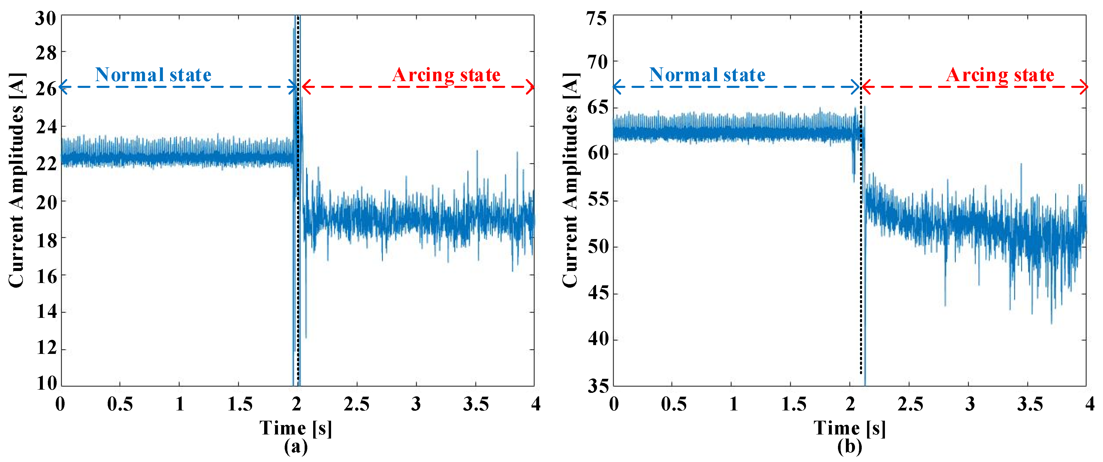
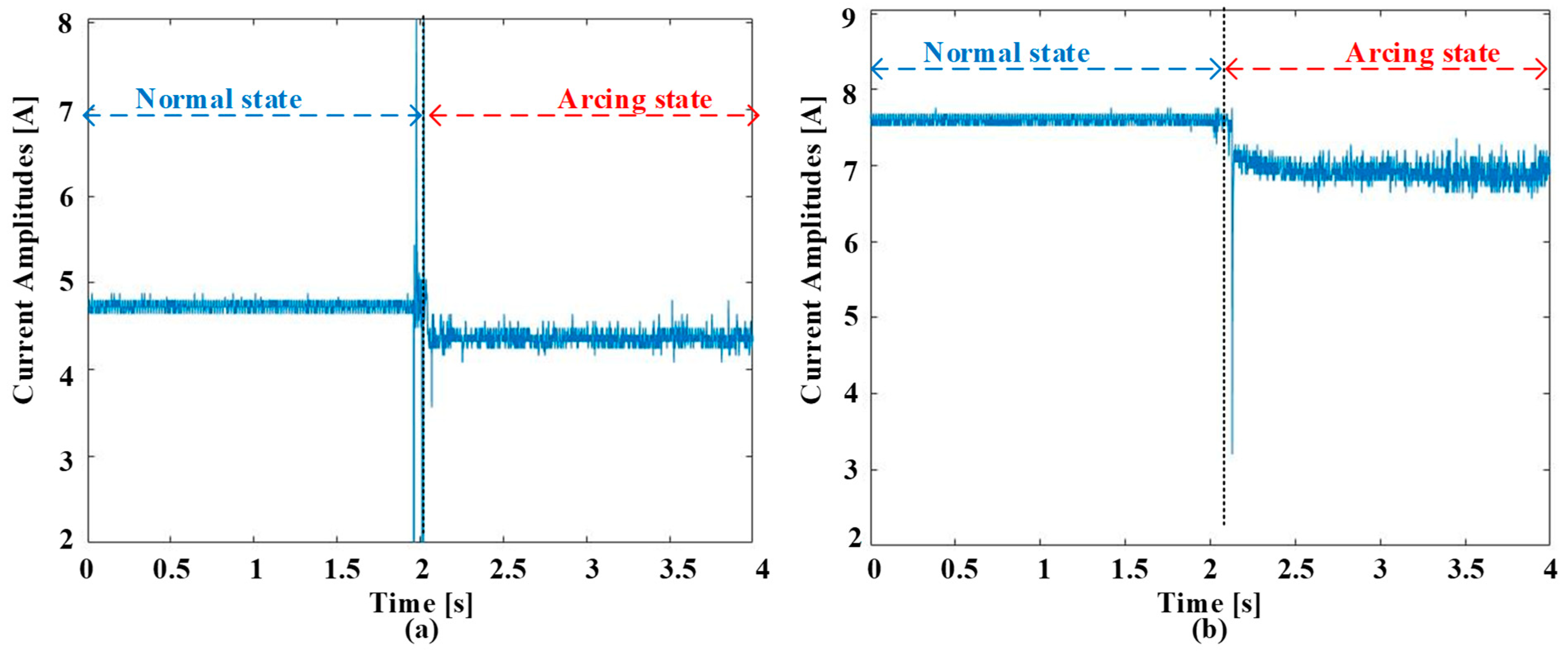
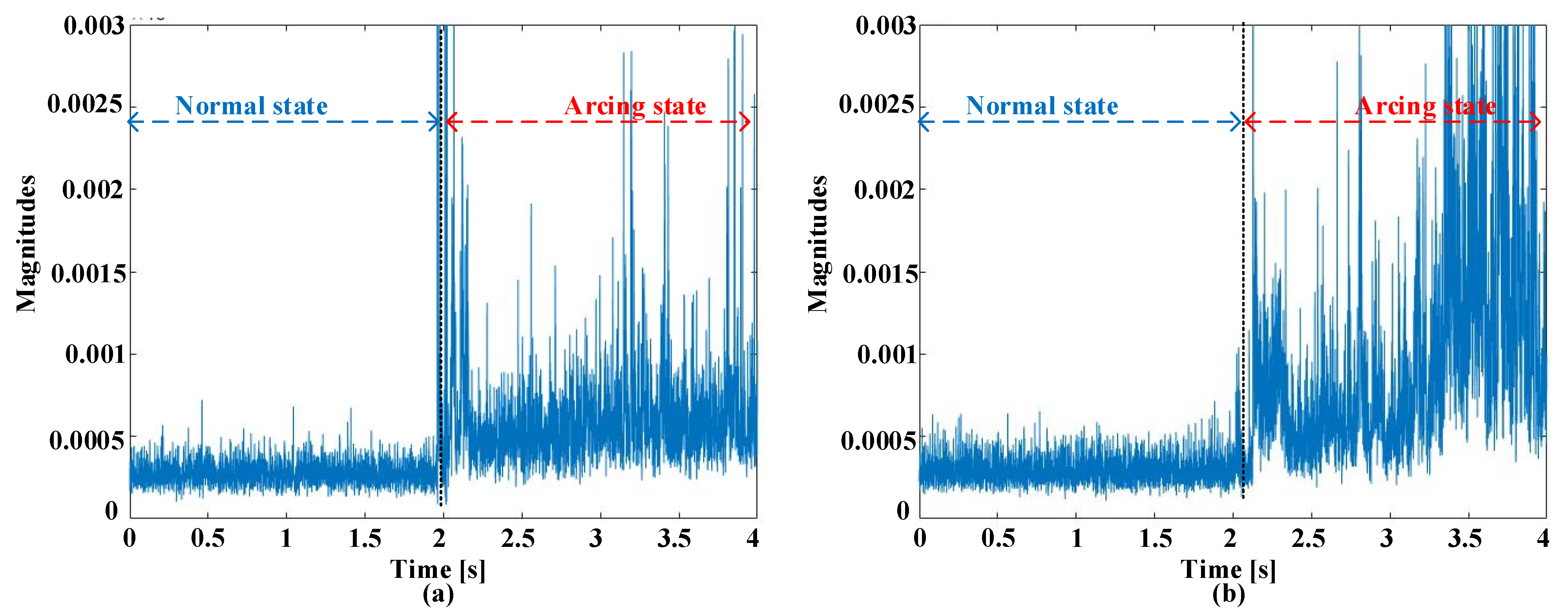
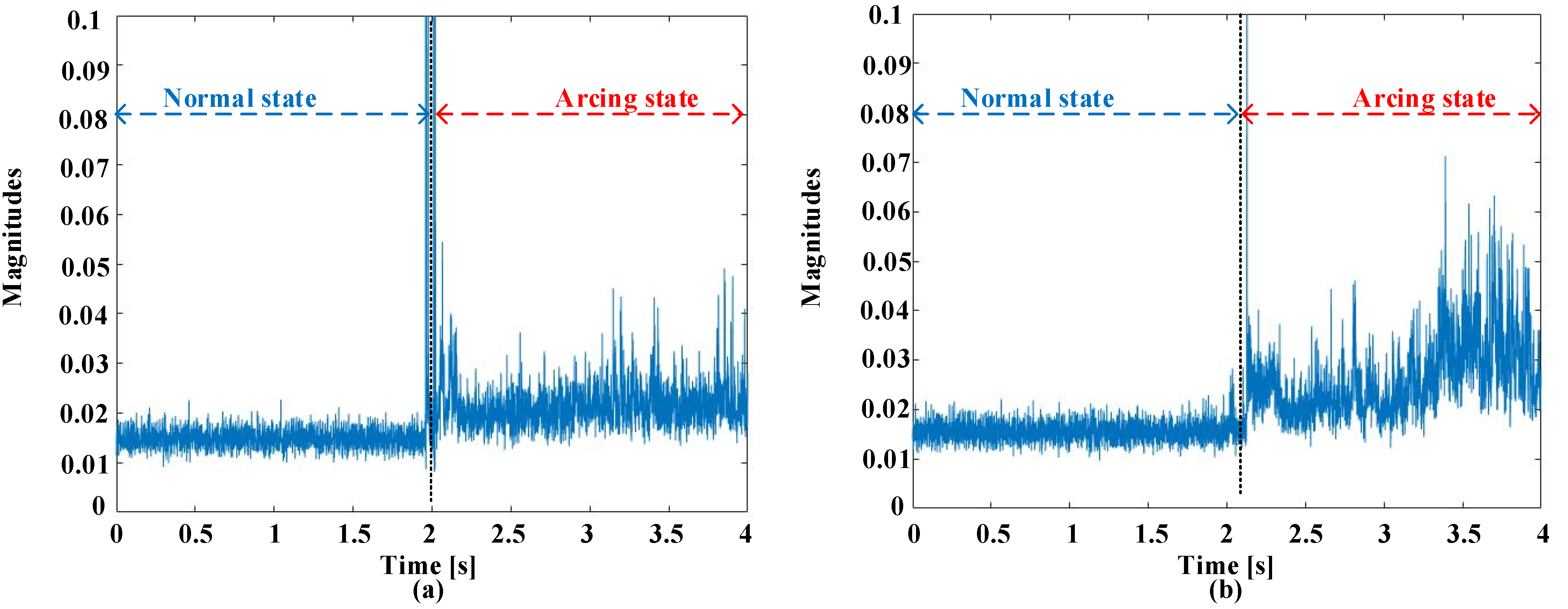
The data, sampled with the rate of 250 kHz, are initially partitioned into separated segments, individually with a period of 0.8 ms. This segmentation facilitates the filtering process and ensures that each data set represents a distinct sampling moment. After partitioning, the filtering process is applied to each segmented data set to extract relevant features. These features include statistical parameters, such as median, average, root mean square (rms), variance, and peak-to-peak. For each data set, these statistical parameters are calculated based on the data points within that specific segment. This process yields a set of feature values corresponding to each segmented data set. Once the feature values are obtained for each segmented data set, they are combined to create a comprehensive data set encompassing all feature values across different sampling moments. This combination involves aggregating the feature values from each segmented data set, resulting in a data set that encapsulates the complete range of feature values over time. Each data point on the curve represents a specific statistical index (e.g., average, median, rms) derived from the aggregated feature values at a particular sampling moment. By plotting these empirical filtering indexes against time, the figure provides insights into how these statistical indexes evolve over the duration of the data set. Figure 4 visually depicts the square average at 5 A and 8 A with the time domain refining where a encompassing a range of three sigma is employed. As depicted in Figure 4, the utilization of square averages results in conspicuous distinctions between the processed signals during various conditions for both the 5 A and 8 A current amplitudes. As a consequence, these signals hold the promise of substantially improving the performance of ILMs in effectively distinguishing between normal and arcing states. Figure 5 illustrates the average values at current amplitudes of 5 A and 8 A. The computation of the average involves summing up all data points within a data set and dividing it by the total number of points. Notably, the average values showcase consistent patterns across normal and arcing states. The normal state exhibits a relatively small change, whereas fluctuations are higher during the arc condition. The fluctuations, however, might not be distinctive enough to serve as a singular discriminative feature between the two states.

Figure 4.
Square average with time domain refining at a 5 kHz switching frequency. (a) 5 A current amplitude. (b) 8 A current amplitude.
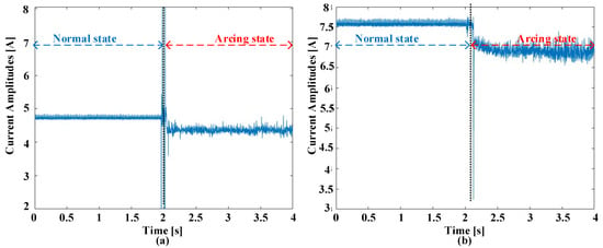
Figure 5.
Averages with time domain refining at a 5 kHz switching frequency. (a) 5 A current amplitude. (b) 8 A current amplitude.
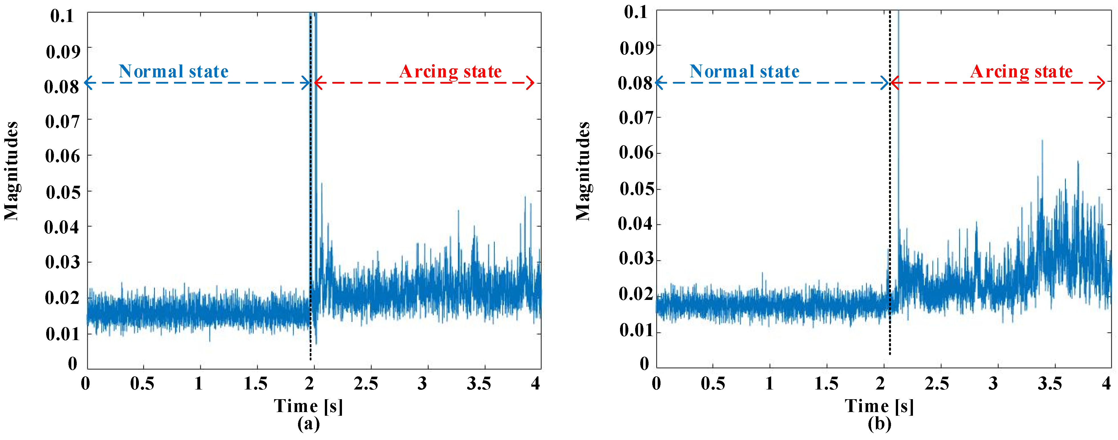
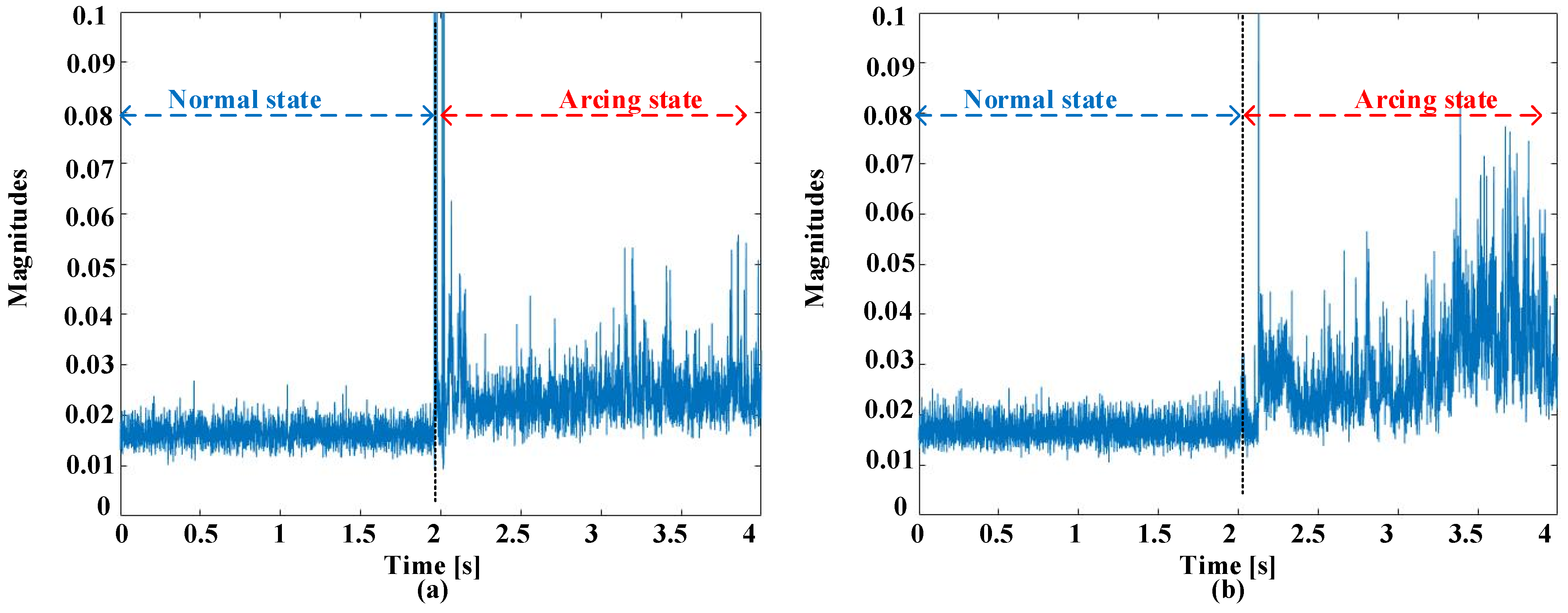
In Figure 6, the median values derived from the signals are presented. The median, which represents the middle point of a data set, offers a robust measure of central tendency. Similar to the average, the median values exhibit discernible differences between normal and arcing states. The stability of the median in the normal state contrasts with the fluctuating nature of the median in the arcing state, providing a potential discriminative feature for classification. Moving to Figure 7, the root mean square (RMS) values obtained from the current signals are shown. The RMS is a measure of the magnitude of a varying quantity, in this context, the signals. The RMS values, akin to the average and median, portray a consistent behavior in the normal state and notable variations during arcing states. The RMS values contribute additional insights into the characteristics of the signals, aiding in the classification process.
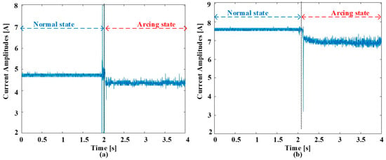
Figure 6.
Medians with time domain refining at a 5 kHz switching frequency. (a) 5 A current amplitude. (b) 8 A current amplitude.
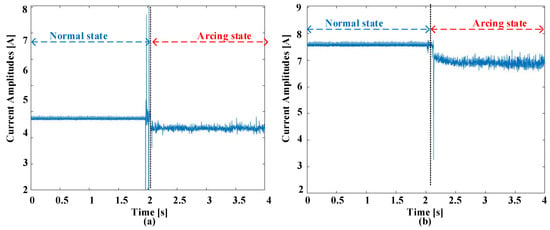
Figure 7.
RMSs with time domain refining at a 5 kHz switching frequency. (a) 5 A current amplitude. (b) 8 A current amplitude.
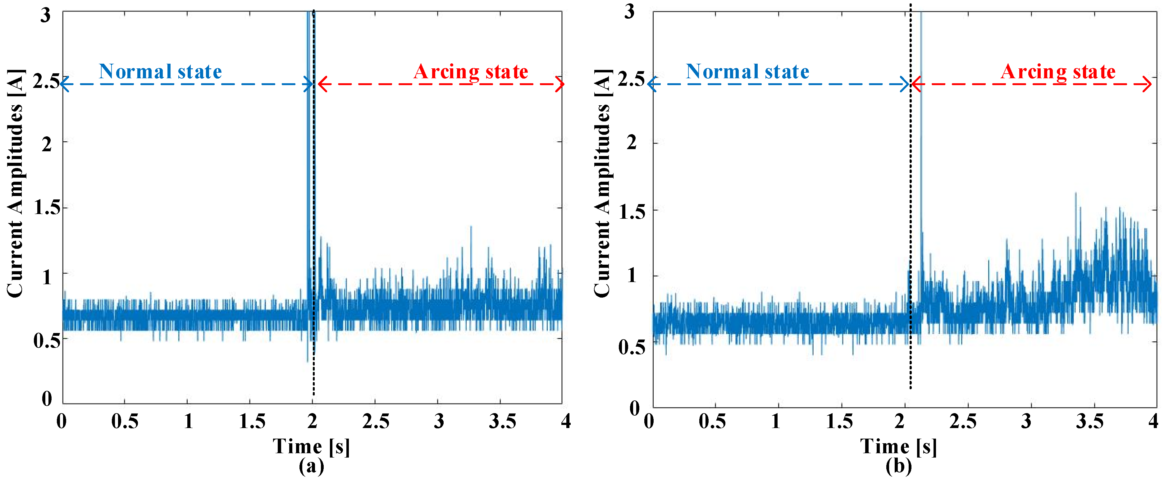
In Figure 8, the peak-to-peak (p2p) values extracted from the current signals are presented. Unlike the average, median, and RMS, the peak-to-peak values do not display as comprehensible differences among various states. The variations in peak-to-peak values for both states are less pronounced, making them less reliable as discriminative features. This suggests that certain signal characteristics might not be as effectively captured by the peak-to-peak measure in the context of arc fault detection. Figure 9 showcases the variance values calculated from the current signals. Variance is a measure of the spread or dispersion of a set of values. Similar to the peak-to-peak values, variance does not distinctly differentiate between normal and arcing states. The intersection in variance quantities for various states indicates that this characteristic aspect alone could not support a satisfactory inequitable capability for precise categorization. In summary, while average, median, and RMS values exhibit consistent patterns aligning with the square averages, peak-to-peak and variance values do not demonstrate vivid gaps in the two states. This nuanced understanding of various signal features contributes to a more comprehensive analysis of the effectiveness of different metrics in the context of DC arc fault detection.

Figure 8.
Peak-to-peaks with time-domain refining at 5 kHz switching frequency. (a) 5 A current amplitude. (b) 8 A current amplitude.
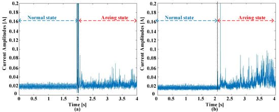
Figure 9.
Variances with time domain refining at a 5 kHz switching frequency. (a) 5 A current amplitude. (b) 8 A current amplitude.
The approach devised for mitigating switching frequency noise is rooted in the frequency domain and is intricately tied to the sampled current [21]. Initially, each segment of the data set undergoes FFT analysis to transform the time domain signal into the frequency domain. This step yields frequency domain features, such as spectral components and harmonics associated with the signal. Following FFT analysis, the filtering technique aims to attenuate or eliminate noise components attributable to the system. After FFT analysis and switching frequency noise filtering, the frequency domain features for each segmented data set are evaluated. These features encompass various statistical parameters similar to those extracted in the time domain, including average, median, rms, peak-to-peak, and variance. Each feature group obtained from the frequency domain analysis represents a specific point in time, reflecting the characteristics of the signal at that particular sampling moment. By combining the feature values obtained from all segmented data sets, a comprehensive data set that captures the behavior of frequency domain features over time is constructed, as shown in Figure 10, Figure 11, Figure 12, Figure 13, Figure 14 and Figure 15. Figure 10 demonstrates the square average with the current amplitudes of both 5 A and 8 A, with a switching frequency set at 5 kHz. This advancement is pivotal in making the arc distortions more conspicuously discernible within the data. It implies that the once obscured arc-related characteristics now stand out more prominently. This improvement in signal property supports substantial capability for fortifying the aspect extraction procedure essential for effective arc identification. Similarly, when the system operates with an increased current of 8 A and 5 kHz, the results remain comparable. These outcomes hold across various scenarios, effectively mitigating switching frequency interferences and ultimately enhancing signal visibility. Consequently, this heightened visibility significantly improves the detectability of arc distortions, ultimately leading to more accurate detection. Figure 11 depicts the average values extracted from the current signals, focusing on current amplitudes of 5 A and 8 A. Averaging involves summing up data points within a data set and dividing by the total number of points. In the context of arc fault detection, the average values present a clear pattern in the two conditions. The normal period exhibits a relatively stable average, while the arcing state introduces fluctuations. These variations, similar to the square average, contribute to the discriminative power of this feature in the classification process.

Figure 10.
Square averages with frequency domain screening at 5 kHz. (a) 5 A current amplitude. (b) 8 A current amplitude.

Figure 11.
Averages with frequency domain screening at 5 kHz. (a) 5 A current amplitude. (b) 8 A current amplitude.
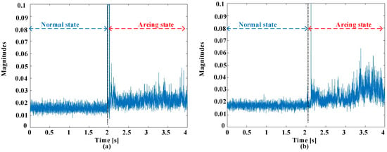
Figure 12.
Medians with frequency domain screening at 5 kHz. (a) 5 A current amplitude. (b) 8 A current amplitude.
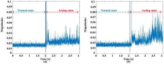
Figure 13.
RMS values with frequency domain screening at 5 kHz. (a) 5 A current amplitude. (b) 8 A current amplitude.

Figure 14.
Peak-to-peak values with frequency domain screening at 5 kHz. (a) 5 A current amplitude. (b) 8 A current amplitude.
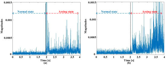
Figure 15.
Variances with frequency domain screening at a 5 kHz switching frequency. (a) 5 A current amplitude. (b) 8 A current amplitude.
In Figure 12, the median values obtained from the signals are illustrated. The median, as a measure of central tendency, is robust in capturing the middle point of a data set. Similar to the average, the median values showcase discernible differences between normal and arcing states. The stability of the median in the normal state and its fluctuations in the arcing state provide valuable information for effective classification. Figure 13 presents the RMS values calculated from the current signals. RMS, as a measure of magnitude, reflects the overall energy content of the signals. The RMS values exhibit patterns similar to the square averages, demonstrating consistency in the normal state and variability in the arcing state.
Moving to Figure 14, the peak-to-peak values extracted from the current signals are shown. Unlike the average, median, and RMS, the peak-to-peak values do not demonstrate comprehensible differences between various states. The variations in peak-to-peak values for both states are less pronounced, suggesting that this feature might not be as efficient in catching the dissimilarities of the two different conditions. Figure 15 illustrates the variance values calculated from the signals. The variance, as a measure of spread, provides insights into the dispersion of values within a data set. Similar to the square average, the variance values present clear differences in the two different conditions. The overlap in variance values for both states indicates the potential of this feature in enhancing the discriminative power for accurate classification. In summary, average, median, rms, and variance values exhibit consistent patterns akin to the square average, contributing to the enhanced visibility of arc distortions. However, peak-to-peak values do not show clear differences in the two different conditions, suggesting limited efficacy in the context of arc fault detection. This detailed analysis of various signal features provides valuable insights for optimizing the detection method.
3. Diagnosis of DC Arc Failure Using Various Indexes with Intelligence Learning Models
This approach commences with the collection of operational data, which are subsequently divided into data sets, each containing 200 data points, equivalent to a duration of 0.8 ms. The choice of 200 data points aligns with practical considerations, such as computational efficiency and memory constraints, making it feasible to process and analyze the data effectively. Overall, with the choice of 200 data points, it is important to consider its implications in relation to the specific requirements and characteristics of the signal being analyzed. The statistics are originally tested at 250 kHz to ensure the capture of fine-grain details. Subsequently, a rigorous process is applied to substitute statistics elements by dropping the outer predefined spans. Time domain square averages are then extracted for each data set. Simultaneously, the data subgroups undergo FFT examination with the output of the FFT operation Both input square averages, originating from both time and frequency domains, are preserved for further analysis. This comprehensive framework spans both training and testing phases, ensuring valuation of the algorithm’s performance under various operative circumstances. The process is systematically applied to various cases, starting with the extraction of square averages in different scenarios. This includes analyzing square averages in the time domain, as well as in the frequency domain. By comparing the performance across these different cases, the optimal approach is determined and subsequently applied to other aspects, such as the median, average, peak-to-peak, rms, and variance. The feature that yields the highest diagnosis rates among all features is identified as the best-performing feature and is consequently prioritized for further analysis and model refinement.
The process of training a machine learning model for an arc identification task involves several key steps. Initially, the data are collected and split into data sets. Next, data preprocessing is performed, including filtering and feature extraction. The data are then divided into training and testing sets. Following this, the machine learning models are selected, and the models are trained on the training data. During training, the model learns the patterns and relationships between the features and labels in the data set. The trained model is evaluated using the testing data, and its performance is assessed using metrics, such as accuracy. In this study, the authors meticulously assembled a training data set comprising 2000 data sets for the training phase and 1000 data sets for each test scenario, covering a range of current amplitudes and switching frequencies. This extensive data set totaled 16,000 data sets for training and 8000 data sets for testing. Each sample within the data set corresponds to a precise moment in time, capturing the electrical signals sampled and recorded at that particular instance. Care was taken to ensure a balanced representation of normal and arcing states within the data set, maintaining a 1:1 ratio between the two states. During the testing phase, this study relied on the accuracy metric as the primary evaluation criterion. The accuracy metric, derived from the confusion matrix, performs by quantifying the proportion of properly categorized instances relative to the entire quantity of instances. The accuracy metric is computed as the correctness detection rate, representing the percentage of precisely forecasted sets out of the entire quantity of examination sets. Precisely forecasted data sets comprise the sum of true positive and true negative instances, while the total number of examination data sets includes true positive, true negative, false positive, and false negative instances. Given the balanced data set distribution and the binary classification task of distinguishing between normal and arcing states, accuracy provides a robust indicator of our model’s classification accuracy.
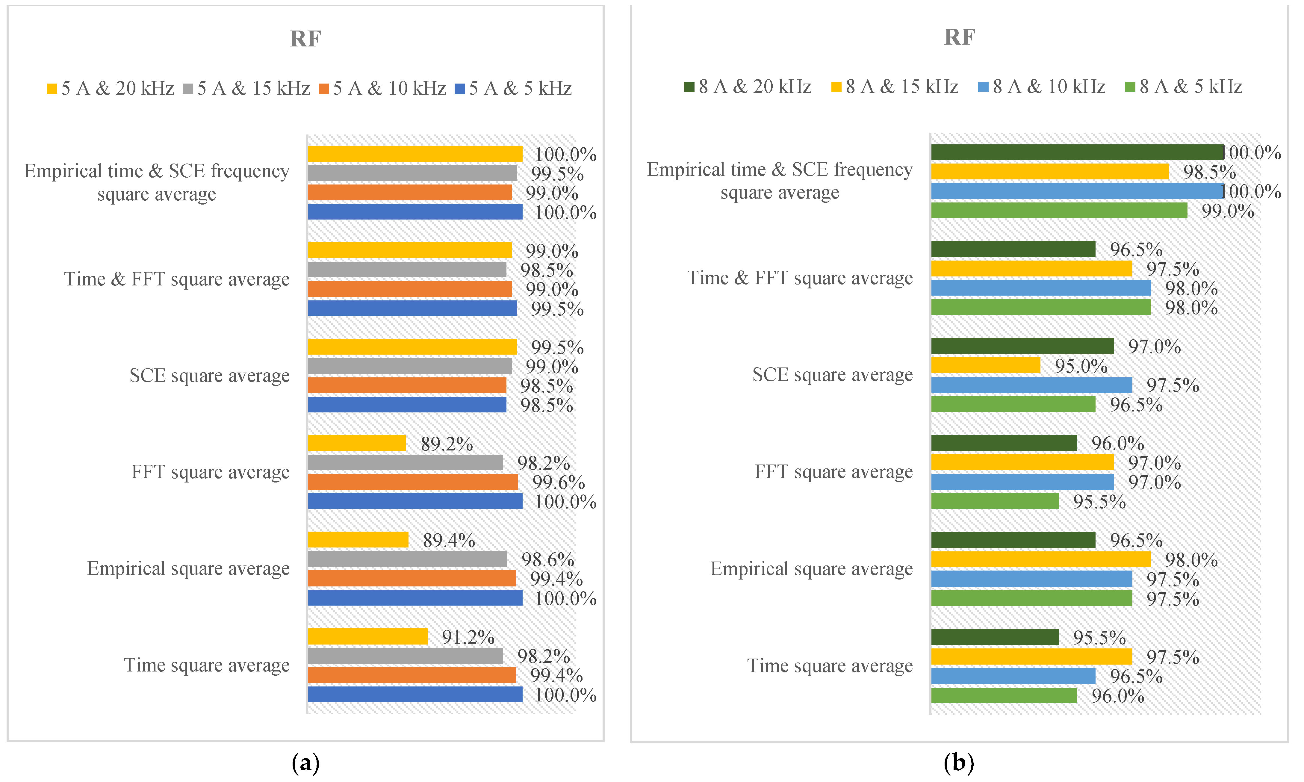
The depiction in Figure 16 showcases the efficacy of arc fault diagnosis in a three-phase inverter across different operational parameters. These outcomes are derived from the SVM algorithm. A noteworthy observation is the superior accuracy achieved with the square average underscoring the efficacy of the filtering process in amplifying the visibility of arc distortions. Moreover, combining square averages in both domains yields a substantial upgrade in the precision of diagnosis when compared to using either the empirical or SCE square averages alone. This enhancement is particularly prominent across all switching rates, signifying the efficiency of this approach in enhancing diagnostic accuracy. It is important to emphasize that, in certain cases, the accuracy achieved by combining the time domain signal square average and FFT square average is similar to the proposed method. However, it should be noted that the proposed approach significantly improves the overall diagnostic accuracy, offering a more robust and effective solution for arc fault detection. This enhanced accuracy is specifically distinct for a current of 8 A, showcasing the robustness and efficiency of this technique across different scenarios. In Figure 17, the authors present a comprehensive analysis of the fault diagnosis performance for an inverter system, investigating a range of operational conditions encompassing various current scales (5 A and 8 A) and various switching rates. This in-depth analysis involves the utilization of an integrated methodology that combines filtering techniques and the RF model. The results of this analysis shed light on the system’s effectiveness in detecting and diagnosing arc faults under diverse scenarios. It is particularly striking to observe that the accuracy of the signal square average consistently outperforms that of the raw signal square average. By preprocessing the data, we effectively amplify the diagnostic potential of the signal, resulting in more pronounced and discernible fault signatures. Furthermore, a significant breakthrough emerges when we combine square averages that have undergone a preprocessing operation.
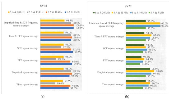
Figure 16.
The diagnosis rates of SVM under various current scales and switching rates. (a) 5 A load. (b) 8 A load.
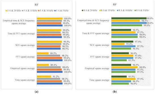
Figure 17.
The diagnosis rates of RF under various current scales and switching rates. (a) 5 A load. (b) 8 A load.
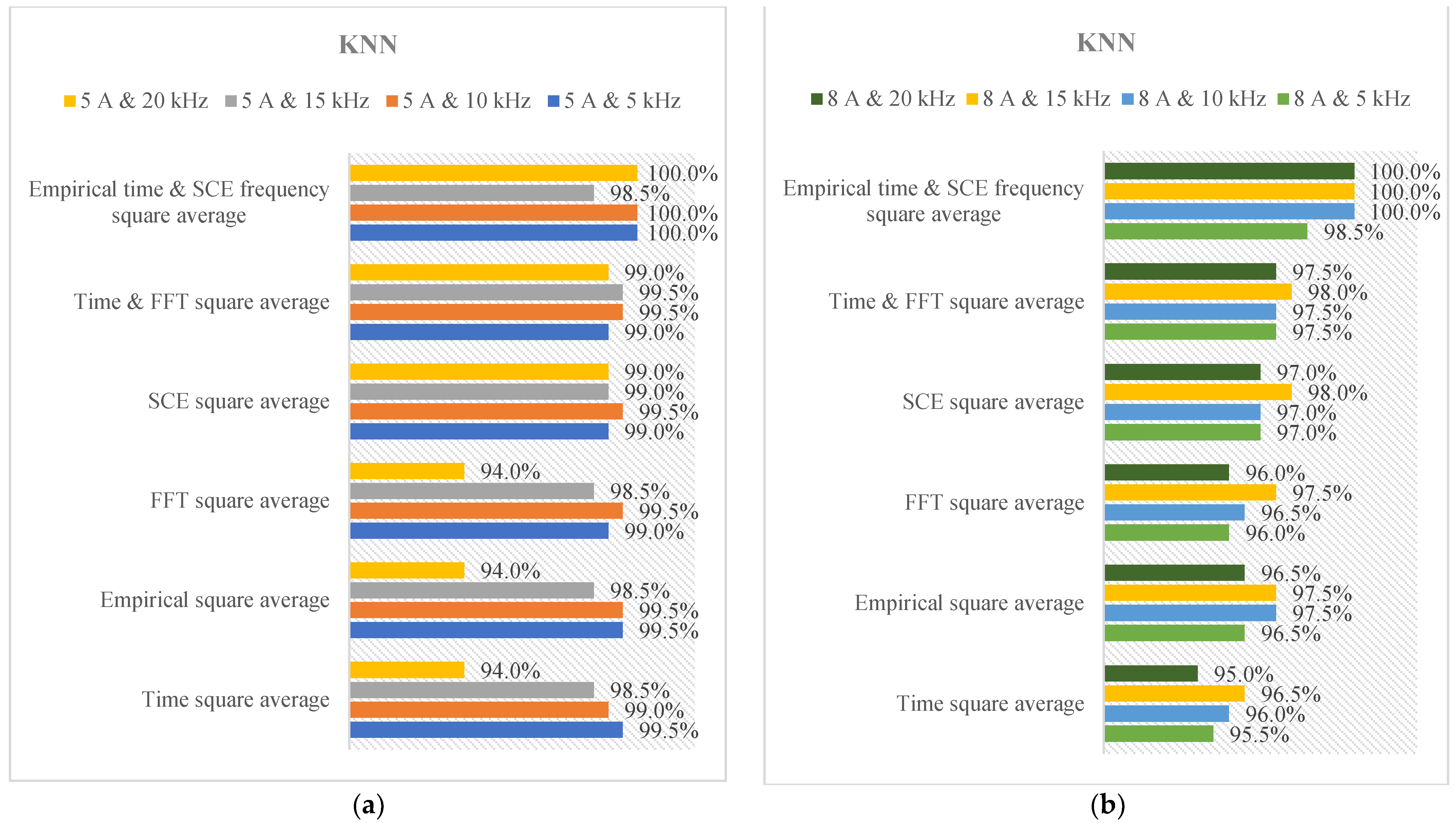
This hybrid approach substantially bolsters the precision of fault diagnosis. In direct comparison to using the square average in isolation, the combined approach excels across the entire spectrum of switching frequencies. This not only reaffirms the value of the filtering process but also highlights the complementary nature of SCE, which enhances the diagnostic accuracy by considering the signal’s complexity. It is worth noting that in specific instances, combining the time domain signal square average with the FFT square average appears to yield accuracy levels similar to those achieved through the proposed methodology. However, what sets the proposed approach apart is its consistent and significant improvement in overall diagnostic accuracy. This improvement is particularly evident when dealing with a higher current of 8 A. The robustness and efficiency of this method in diagnosing arcing failures across diverse scenarios become evident, making it a superior choice for enhancing diagnostic precision. Moreover, the precision achieved with the proposed approach outperforms other input combinations with remarkable accuracy, underscoring its effectiveness in arc fault detection. In Figure 18, we present a comprehensive and meticulous examination of the performance of an arc fault diagnosis system within the context of a three-phase inverter setup. This investigation encompasses a spectrum of operational scenarios, spanning altered scales (5 A and 8 A) and an array of switching rates. This detailed analysis employs an integrated methodology that harmoniously combines empirical filtering, SCE, and the KNN algorithm. The findings that emerge from this thorough evaluation illuminate the system’s prowess in the detection and diagnosis of arc faults across a diverse range of operational contexts. Notably, a prominent and consistent trend arises throughout the analysis: the accuracy of the filtered signal square average consistently surpasses that of the raw signal square average. This observation underscores the invaluable role of the filtering procedure in accentuating the discernibility and unequivocal identification of arcing alterations within the signal. By subjecting the data to empirical filtering, we significantly amplify the diagnostic potential of the signal, leading to the emergence of more pronounced and distinctly discernible fault signatures.
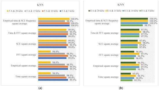
Figure 18.
The diagnosis rates of KNN under various current scales and switching rates. (a) 5 A load. (b) 8 A load.
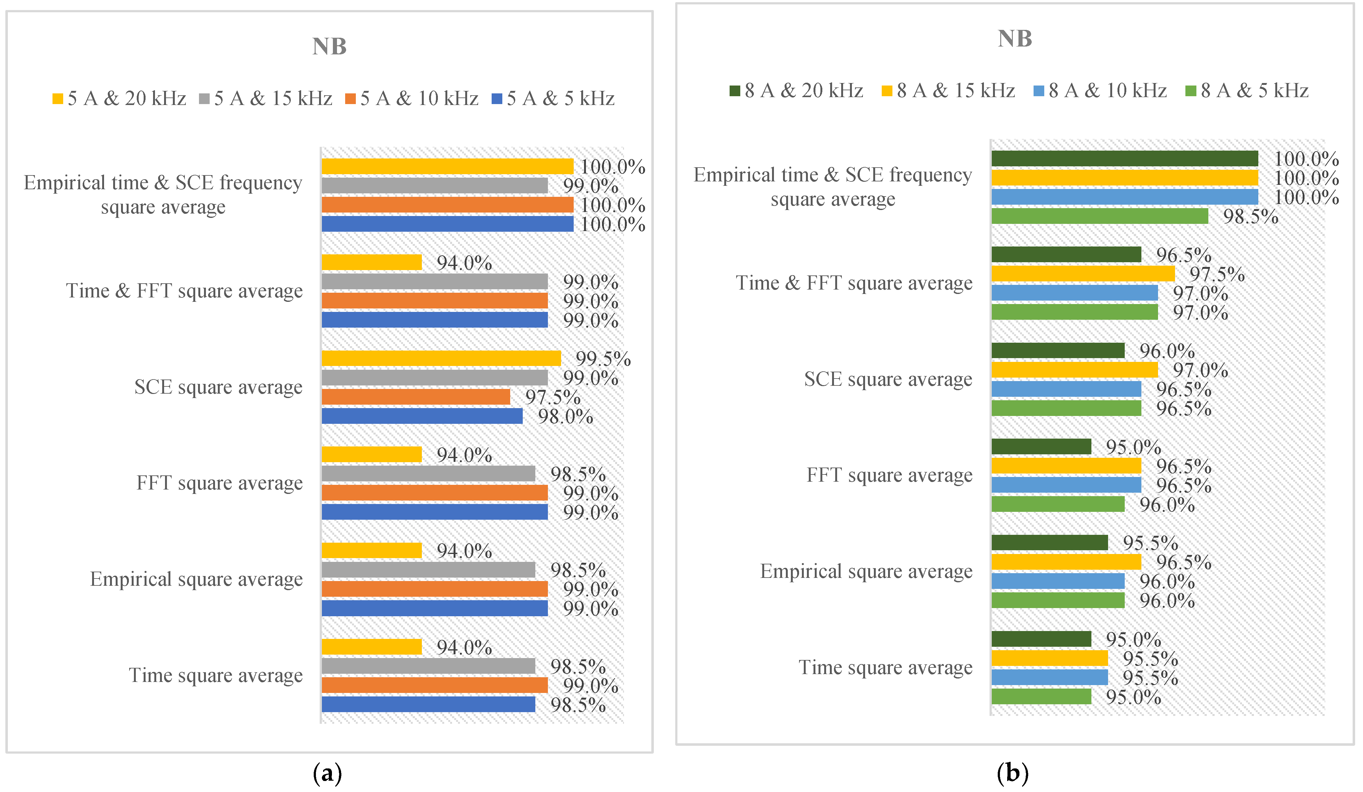
Moreover, a pivotal advancement materializes when we amalgamate square averages that have undergone preprocessing with both empirical filtering and SCE. This hybrid approach markedly bolsters the precision of arcing diagnosis. In direct comparison to the utilization of either the empirical or SCE square average in isolation, the combined approach consistently excels across the entire spectrum of switching frequencies. This outcome reaffirms the intrinsic value of the filtering process and accentuates the complementarity of SCE in terms of enhancing diagnostic accuracy, considering the signal’s complexity. This improvement is particularly evident in scenarios involving higher current amplitudes, such as 8 A. This underscores the robustness and efficiency of this method in diagnosing arcing failures across diverse operational settings, establishing it as the preferred choice for enhancing diagnostic precision. In Figure 19, we present a meticulous and all-encompassing examination of the performance of an arc fault diagnosis system implemented within the context of a three-phase inverter configuration. This comprehensive investigation spans a gamut of operational scenarios, including varying current amplitudes (5 A and 8 A) and an assortment of switching frequencies. This detailed analysis is underpinned by an integrated methodology that seamlessly harmonizes empirical filtering, SCE, and the NB algorithm. The outcomes emerging from this exhaustive evaluation shed light on the system’s remarkable capabilities in the domain of detecting and diagnosing arc faults across a wide spectrum of operational conditions. A conspicuous and recurring trend permeates this extensive analysis: the accuracy of the filtered signal square average consistently outperforms that of the raw signal square average. This observation accentuates the invaluable role of the filtering procedure in developing the discernibility and unequivocal identification of arc distortions embedded within the signal. By subjecting the data to empirical filtering, we conspicuously amplify the diagnostic potential of the signal, thereby inducing the emergence of more pronounced and distinctly discernible fault signatures. Furthermore, a significant milestone is achieved when we amalgamate square averages that have undergone preprocessing with both empirical filtering and SCE.

Figure 19.
The diagnosis rates of NB under various current scales and switching rates. (a) 5 A load. (b) 8 A load.
This hybrid approach substantially bolsters the precision of failure diagnosis. In direct comparison to the use of either the empirical or SCE square average in isolation, the combined approach consistently excels across the entire spectrum of switching frequencies. This outcome not only reaffirms the intrinsic value of the filtering process but also underscores the complementarity of SCE in terms of enhancing diagnostic accuracy, particularly with regards to the complexity of the signal. This enhancement is especially prominent in scenarios involving higher current amplitudes, such as 8 A, underscoring the robustness and efficacy of the proposed technique in diagnosing arc faults across diverse operational settings. This firmly establishes it as the preferred choice for enhancing diagnostic precision in a wide array of situations. In Figure 20, we present an exhaustive and comprehensive analysis of the performance of an arc fault diagnosis system, operating within the framework of a three-phase inverter setup. This in-depth investigation encompasses a wide spectrum of operational scenarios, incorporating variable amplitudes (5 A and 8 A) and an array of switching rates. This intricate analysis is underpinned by an integrated methodology that harmoniously blends empirical filtering, SCE, and the DT algorithm. The outcomes arising from this thorough evaluation shed illuminating insights into the system’s formidable capabilities in the realm of detecting and diagnosing arc faults under a diverse range of operational contexts. A prominent and consistent trend surfaces throughout this extensive analysis: the accuracy of the filtered signal square average consistently surpasses that of the raw signal square average. This observation underscores the invaluable role of the filtering process in accentuating the visibility and unequivocal identification of arc distortions within the signal. By subjecting the data to empirical filtering, we significantly amplify the diagnostic potential of the signal, leading to the emergence of more pronounced and distinctly discernible fault signatures.
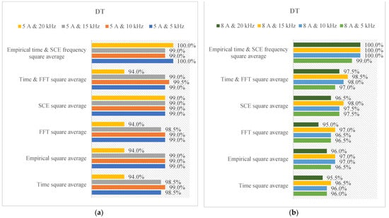
Figure 20.
The diagnosis rates of DT under various current scales and switching rates. (a) 5 A load. (b) 8 A load.
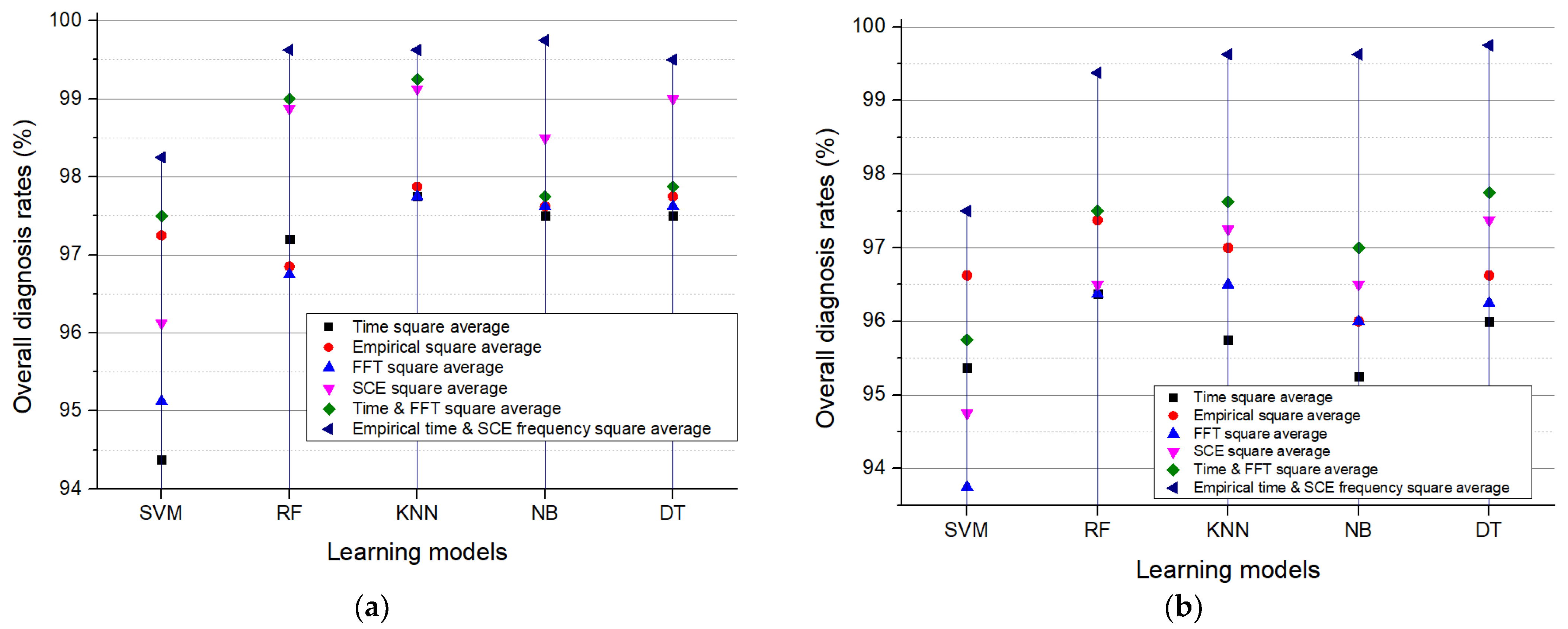
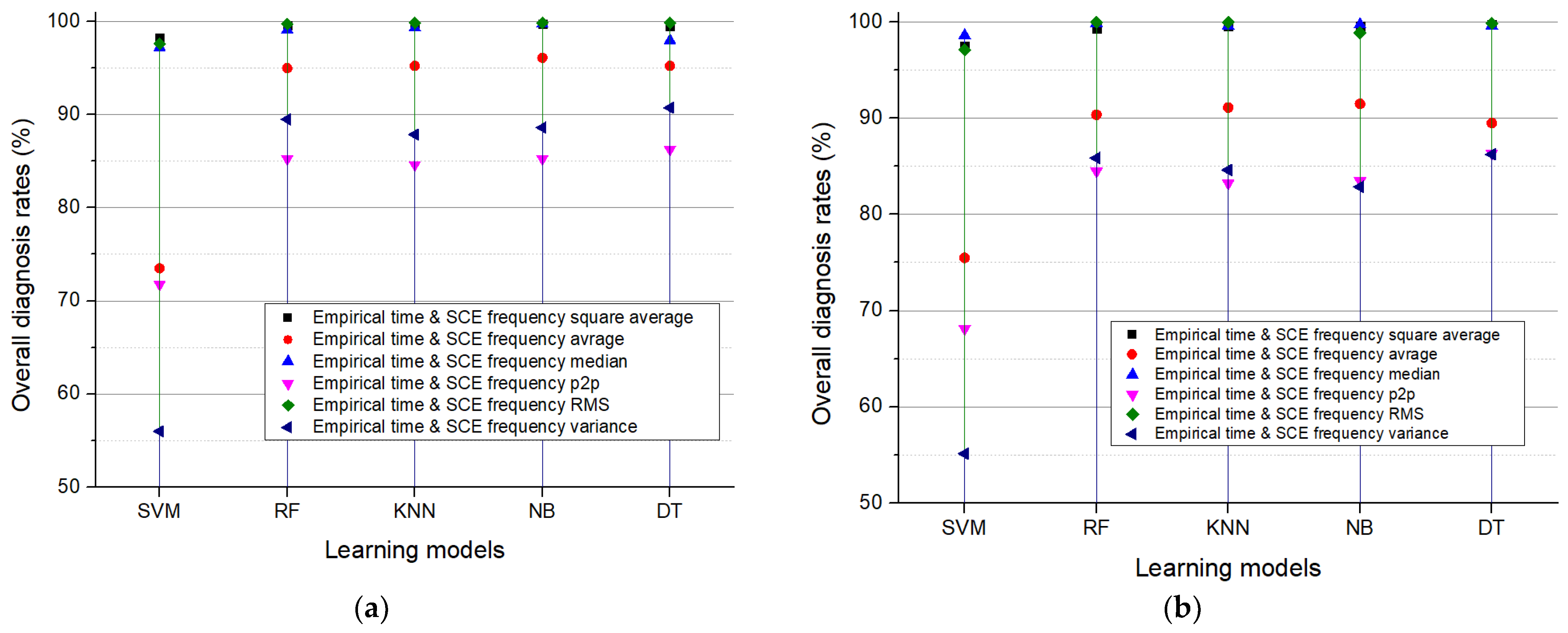
Figure 21 provides results of the accuracy of ILMs in the exciting field of DC arcing failure diagnosis using various features and different models. This observation emphasizes that the preprocessing techniques complement each other effectively, enhancing diagnostic accuracy. Additionally, it is worth noting that the accuracy achieved using the combination of time domain square average and frequency FFT square average closely align with the proposed scheme. This result suggests that traditional methods that do not require advanced preprocessing can still provide competitive accuracy, particularly in specific scenarios. This indicates that while advanced techniques, like empirical filtering and SCE, offer significant benefits, there is still value in more straightforward approaches. Within the domain of ILMs, RF and KNN consistently stand out as the top performers, irrespective of the input or switching rates. This incredible reliability emphasizes the strong abilities of ILMs for DC arcing failure diagnosis. Their adaptability and accuracy in providing diagnoses across diverse conditions render them highly suitable for arc fault detection systems. In summary, the diagnostic results are both evident and compelling. The proposed approach for DC arc fault diagnosis consistently surpasses various alternative techniques, underscoring its potential to enhance diagnosis accuracy across a spectrum of scenarios. The integration of empirical filtering and SCE, coupled with versatile learning models, such as RF and KNN, presents a formidable strategy for DC arc fault detection. This study constitutes a significant contribution to the realm of electrical system safety, addressing a critical concern in applications where DC arc faults pose substantial risks. The results confirm the viability of these approaches and lay the foundation for more reliable and accurate arc fault detection systems, ultimately enhancing safety and reducing the potential for catastrophic electrical events. The comprehensive diagnostic procedures applied to square averages were replicated for additional features, including average, median, p2p, RMS, and variance. Through extensive analysis, it is clear that the combination of the empirical filtering square average with the SCE square average consistently outperforms alternative configurations across diverse input scenarios. The intricate details of this comparison are omitted for brevity, focusing on the collective superiority of these combined square averages. In Figure 22, an exhaustive overview of the accuracy of ILMs is presented, utilizing various input features in the demanding area of DC arcing failure diagnosis. The performance evaluation indicates that the square average, median, and RMS features exhibit superior capabilities in diagnosing arc faults compared to p2p and variance features. These findings underscore the effectiveness of this diagnosis approach, consistently surpassing alternative techniques and demonstrating its potential to enhance diagnostic accuracy across a spectrum of scenarios. The results not only validate the viability of the employed approaches but also establish a robust foundation for the development of more reliable and accurate arc fault detection systems. This advancement holds significant promise for improving overall safety in electrical systems and mitigating the risks associated with potentially catastrophic electrical events. The thorough exploration and comparison of various features contribute valuable insights to the refinement and optimization of future diagnostic methodologies in the context of DC arc fault detection. The developed features in this paper showed better performance in comparison with previous approaches to detect the DC arc failures using some catalogue [19]. The previous approach in [19] used a few simple features, which were integral, kurtosis, and Shannon entropy, to detect the DC arc faults. On the other hand, this work proposed new features different than those used in the previous paper, which are the square average, the average, the median, the rms, the peak-to-peak, and the variance values, to find out which one can be the most effective features to detect DC arc failure. In this paper, the new features, such as the square average, the rms, and the median values among the various features, which can detect the DC arc failure more accurately than the simple features of the previous paper. Furthermore, this paper addressed which artificial learning model can be better in conjunction with the various developed features, and the K-nearest neighbor (KNN) was found out to show the best accuracy. In addition, the proposed setup includes an arc generator designed to produce well-defined arcs, as evidenced by the distinct patterns observed in Figure 2, which depict the differences between different states. These patterns serve as valuable indicators for identifying and characterizing fault events within the electrical system. However, the system’s performance in scenarios involving the superimposition of a normal state with a state of low-intensity arcing is noteworthy. In such cases, where low-intensity arcing may occur concurrently with normal operating conditions, the detection of arcing events becomes more challenging due to the presence of subtle variations in the electrical signals. To address this challenge, this proposed detection method leverages advanced signal processing techniques and feature extraction algorithms to discern subtle changes in the waveform characteristics associated with low-intensity arcing. By analyzing the temporal and spectral features of the electrical signals, this method is capable of detecting and distinguishing between different states, even in scenarios where the intensity of the arcing event is relatively low. Furthermore, the use of machine learning algorithms enhances the system’s ability to identify patterns indicative of arcing activity, allowing for the reliable detection of fault events amidst varying operating conditions. Through rigorous testing and validation procedures, we have demonstrated the effectiveness of our detection method in accurately identifying and classifying arcing events. Despite the challenges posed by the superimposition of normal and low-intensity arcing states, this proposed system is designed to address these challenges through its robust signal processing techniques and machine learning capabilities. This approach offers a reliable solution for detecting and mitigating the risks associated with arc faults in electrical systems.
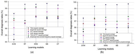
Figure 21.
The overall detection rates of ILMs under various type of square average. (a) 5 A load. (b) 8 A load.
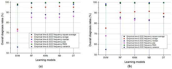
Figure 22.
The overall detection rates of ILMs under various inputs. (a) 5 A load. (b) 8 A load.
4. Conclusions
This pioneering study introduces a novel strategy for addressing the intricate challenge of DC arc fault detection. In this paper, notably, RF and KNN emerge as top-performing ILMs, consistently exhibiting robust diagnostic capabilities under different operating conditions. The comparison between features highlights the superior performance of ILMs using various input features in the demanding realm of DC arc fault detection. Specifically, the square average, median, and RMS features stand out as exceptional performers, outclassing peak-to-peak (p2p) and variance features. This collective success underscores the considerable potential of the proposed approach to enhance safety and reliability in electrical systems. Beyond laboratory settings, its real-world impact is tangible, addressing critical concerns in industrial settings and data centers. By laying the groundwork for more robust, precise, and dependable arc fault detection, this research contributes promising strides towards safety and reliability in diverse critical electrical systems.
Author Contributions
Conceptualization, S.K.; methodology, S.K. and S.C.; software, H.-L.D.; validation, H.-L.D.; formal analysis, S.K.; investigation, H.-L.D.; resources, S.K.; data curation, H.-L.D.; writing—original draft preparation, H.-L.D.; writing—review and editing, S.K. and S.C.; visualization, H.-L.D.; supervision, S.K.; project administration, S.K.; funding acquisition, S.K. All authors have read and agreed to the published version of the manuscript.
Funding
This work was supported by the National Research Foundation of Korea (NRF) grant funded by the Korea government (MSIT) (2020R1A2C1013413) and the Korea Institute of Energy Technology Evaluation and Planning (KETEP) and the Ministry of Trade, Industry & Energy (MOTIE) of the Republic of Korea (No. 20214000000280).
Data Availability Statement
Data are contained within the article.
Conflicts of Interest
The authors declare no conflicts of interest.
References
- Lee, S.; Kim, H. A study on low-voltage DC circuit breakers. In Proceedings of the 2013 IEEE International Symposium on Industrial Electronics, Taipei, Taiwan, 28–31 May 2013; pp. 1–6. [Google Scholar]
- Gammon, T.; Lee, W.J.; Zhang, Z.; Johnson, B.C. A review of commonly used DC arc models. IEEE Trans. Ind. Appl. 2015, 51, 1398–1407. [Google Scholar] [CrossRef]
- Klement, K. DC arc flash studies for solar photovoltaic systems: Challenges and recommendations. IEEE Trans. Ind. Appl. 2015, 51, 4239–4244. [Google Scholar] [CrossRef]
- Zhao, S.; Wang, Y.; Niu, F.; Zhu, C.; Xu, Y.; Li, K. A Series DC Arc Fault Detection Method Based on Steady Pattern of High-Frequency Electromagnetic Radiation. IEEE Trans. Plasma Sci. 2019, 47, 4370–4377. [Google Scholar] [CrossRef]
- Park, S.Y.; Choi, H.S. Operation characteristics of DC circuit breaker using arc induction technique according to the magnetism of the superconducting magnet. J. Electr. Eng. Technol. 2024, 19, 845–850. [Google Scholar] [CrossRef]
- Georgijevic, N.L.; Jankovic, M.V.; Srdic, S.; Radakovic, Z. The detection of series arc fault in photovoltaic systems based on the arc current entropy. IEEE Trans. Power Electron. 2016, 31, 5917–5930. [Google Scholar] [CrossRef]
- Chae, S.; Park, J.; Oh, S. Series DC arc fault detection algorithm for DC microgrids using relative magnitude comparison. IEEE J. Emerg. Sel. Top. Power Electron. 2016, 4, 1270–1278. [Google Scholar] [CrossRef]
- Ahn, J.-B.; Jo, H.-B.; Ryoo, H.-J. Real-Time DC Series Arc Fault Detection Based on Noise Pattern Analysis in Photovoltaic System. IEEE Trans. Ind. Electron. 2023, 70, 10680–10689. [Google Scholar] [CrossRef]
- Khamkar, A.; Patil, D.D. Arc fault and flash signal analysis of DC distribution system sing artificial intelligence. In Proceedings of the 2020 International Conference on Renewable Energy Integration into Smart Grids: A Multidisciplinary Approach to Technology Modelling and Simulation (ICREISG), Bhubaneswar, India, 14–15 February 2020; pp. 10–15. [Google Scholar]
- Dang, H.-L.; Kwak, S.; Choi, S. Different Domains Based Machine and Deep Learning Diagnosis for DC Series Arc Failure. IEEE Access 2021, 9, 166249–166261. [Google Scholar] [CrossRef]
- Ni, Y.; Zhang, X.; Chen, Q.; Huang, Y.; Wang, Q. Performance comparison of surface-inset machines with two layer equal/unequal magnet-arc halbach magnets. J. Electr. Eng. Technol. 2024, 19, 845–850. [Google Scholar] [CrossRef]
- Xiong, Q.; Feng, X.; Gattozzi, A.L.; Liu, X.; Zheng, L.; Zhu, L.; Ji, S.; Hebner, R.E. Series Arc Fault Detection and Localization in DC Distribution System. IEEE Trans. Instrum. Meas. 2020, 69, 122–134. [Google Scholar] [CrossRef]
- Yao, X.; Wang, J.; Schweickart, D.L. Review and recent developments in DC arc fault detection. In Proceedings of the 2016 IEEE International Power Modulator and High Voltage Conference (IPMHVC), San Francisco, CA, USA, 6–9 July 2016; pp. 467–472. [Google Scholar]
- Wang, Y.; Zhang, F.; Zhang, S. A new methodology for identifying arc fault by sparse representation and neural network. IEEE Trans. Instrum. Meas. 2018, 67, 2526–2537. [Google Scholar] [CrossRef]
- Laldingliana, J.; Biswas, P.K. Artificial intelligence based fractional order PID control strategy for active magnetic bearing. J. Electr. Eng. Technol. 2022, 17, 3413–3426. [Google Scholar] [CrossRef]
- Uriarte, F.M.; Gattozzi, A.L.; Herbst, J.D.; Estes, H.B.; Hotz, T.J.; Kwasinski, A.; Hebner, R.E. A DC arc model for series faults in low voltage microgrids. IEEE Trans. Smart Grid 2012, 3, 2063–2070. [Google Scholar] [CrossRef]
- Som, S.; Samantaray, S.R. Wavelet based fast fault detection in LVDC micro-grid. In Proceedings of the 2017 7th International Conference on Power Systems (ICPS), Pune, India, 21–23 December 2017; pp. 87–92. [Google Scholar]
- Dang, H.-L.; Kwak, S.; Choi, S. DC Series Arc Fault Diagnosis Scheme Based on Hybrid Time and Frequency Features Using Artificial Learning Models. Machines 2024, 12, 102. [Google Scholar] [CrossRef]
- Gu, J.-C.; Lai, D.-S.; Wang, J.-M.; Huang, J.-J.; Yang, M.-T. Design of a DC Series Arc Fault Detector for Photovoltaic System Protection. IEEE Trans. Ind. Appl. 2019, 55, 2464–2471. [Google Scholar] [CrossRef]
- Dang, H.-L.; Kwak, S.; Choi, S. DC Series Arc Failure Diagnosis using Artificial Machine Learning with Switching Frequency Component Elimination Technique. IEEE Access 2023, 11, 119584–119595. [Google Scholar] [CrossRef]
- UL 1699B; Outline of Investigation for Photovoltaic (PV) dc Arc-Fault Circuit Protection, Issue 2. Underwriters Laboratories, Inc.: Northbrook, IL, USA, 2013.
- Boser, B.E.; Guyon, I.M.; Vapnik, V.N. A training algorithm for optimal margin classifiers. In Proceedings of the Fifth Annual Workshop on Computation Learning Theory (COLT’92), Pittsburgh, PA, USA, 27–29 July 1992; pp. 144–152. [Google Scholar]
- Dang, H.-L.; Kwak, S.; Choi, S. Empirical Filtering-Based Artificial Intelligence Learning Diagnosis of Series DC Arc Faults in Time Domains. Machines 2023, 11, 968. [Google Scholar] [CrossRef]
- Cover, T.; Hart, P. Nearest neighbor pattern classification. IEEE Trans. Inf. Theory 1967, 13, 21–27. [Google Scholar] [CrossRef]
- Breiman, L.; Friedman, J.; Olshen, R.; Stone, C. Classification and Regression Trees; ser. Statistics/Probability Series; Wadsworth and Brooks: Belmont, CA, USA, 1984. [Google Scholar]
- Dang, H.-L.; Kwak, S.; Choi, S. Identifying DC Series and Parallel Arcs Based on Deep Learning Algorithms. IEEE Access 2022, 10, 76386–76400. [Google Scholar] [CrossRef]
- Breiman, L. Random forests. Mach. Learn. 2001, 45, 5–32. [Google Scholar] [CrossRef]
- Langley, P.; Iba, W.; Thompson, K. An analysis of Bayesian classifiers. In Proceedings of the 10th National Conference on Artificial Intelligence, San Jose, CA, USA, 12–16 July 1992; pp. 223–228. [Google Scholar]
Disclaimer/Publisher’s Note: The statements, opinions and data contained in all publications are solely those of the individual author(s) and contributor(s) and not of MDPI and/or the editor(s). MDPI and/or the editor(s) disclaim responsibility for any injury to people or property resulting from any ideas, methods, instructions or products referred to in the content. |
© 2024 by the authors. Licensee MDPI, Basel, Switzerland. This article is an open access article distributed under the terms and conditions of the Creative Commons Attribution (CC BY) license (https://creativecommons.org/licenses/by/4.0/).


