Abstract
This study introduced a novel path-following controller tailored to electric vehicles equipped with a steer-by-wire system, i.e., the steering angle of the vehicle was defined by an electrical actuator. The control objective was to force the proper steering angle of the vehicle, which permits following a desired path. The system presupposed that an external algorithm that utilized sensor data provided the lateral movement references while maintaining a steady longitudinal velocity for the vehicle. The proposed control scheme was based on a robust sliding mode steering controller to manage the vehicle’s lateral movement. Furthermore, a brushless DC (BLDC) motor was considered as the steering actuator, which was controlled by a field-oriented controller (FOC), which was based on four internal proportional–integral (PI) control loops for precise steering actuation. To assess the performance of the proposed control scheme, numerical simulations were obtained, which demonstrated its effectiveness in achieving the control objective.
1. Introduction
Advanced driving assistance systems are evolving rapidly, with the ultimate goal to achieve full self-driving vehicles that can be applied in many fields and industries, such as transportation and mobility, surveillance, healthcare, agriculture, construction, and manufacturing. One of the advantages of these systems is the improvement of the safety of the passengers and operators of machinery on roads since these systems do not get tired or commit unsafe behaviors or risky actions.
We can mention some automotive systems intended to keep a vehicle on track or to assist the driver in this task. Some of these systems are commercially known as lane-keeping assist systems (LKASs), whose objective is to help the driver to maintain the vehicle in its respective lane; lane departure avoidance (LDA) SAE L0 (no automation), which corrects the steering angle of the vehicle to prevent departure from a specific lane; the emergency lane-keeping system (ELKS), which is an adaptive application to reduce the effort required by the driver to keep their vehicle centered in the lane; the lane-change system SAE L2 (partially automated system), which, after an initial command or confirmation by the driver, applies automatic steering to move the vehicle to an adjacent lane; and, of course, the full automation driving from SAE L4 to L5.
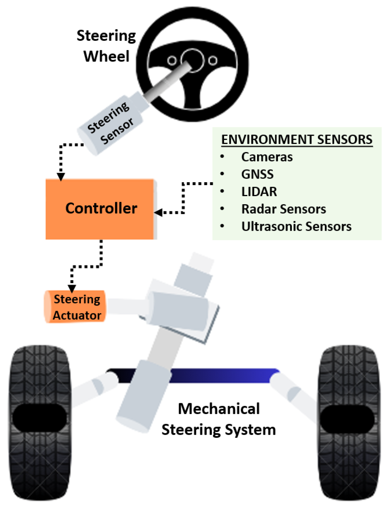
These systems provide different levels of autonomy to the vehicle and are based on automatically controlling its inputs, such as the steering angle, traction torque, and braking. Usually, a path-following scheme for a vehicle considers the integration of a steer-by-wire system, as depicted in Figure 1, which represents a simplified version of the real system. In this case, the steering wheel does not have a physical connection to the mechanical steering system. Instead, a controller monitors the steering wheel using a steering sensor and determines how the mechanical system is modified by means of a steering actuator. Furthermore, the controller receives information about the environment of the vehicle from a set of sensors, such as cameras, a global navigation satellite system (GNSS), LIDAR, and radar and ultrasonic sensors. It is important to note that the performance of the global control scheme fundamentally depends on the accuracy and precision of the environment sensors and the algorithms that permit monitoring the environment and, in particular, the road. This represents a very promising research area in the field of autonomous vehicles, but it is not within the scope of the presented work.

Figure 1.
Overall control architecture for path following with different levels of autonomy.
The controller block in Figure 1 was designed using different approaches. For instance, in [1], two nonlinear controllers were developed for autonomous vehicles, while ref. [2] presents a path-following control algorithm for a vehicle. Some controller design techniques include adaptive control [3], optimal control schemes [4,5], algorithms based on model predictive control (MPC) [6,7], and controllers using artificial intelligence algorithms as reinforcement learning [8], among others, such as [9,10,11,12]. On the other hand, other works were focused on taking advantage of the robustness of the sliding mode control (SMC) algorithms, as any vehicle will encounter the effect of disturbances due to external and internal factors, such as wind, road irregularities, noise in sensor data, model uncertainties, and parameter variations. Sliding mode control is a nonlinear control technique that aims to compensate for the discrepancies that exist between reality and the mathematical model used to analyze and design the control algorithm. Essentially, the SMC consists of switching the inputs of a system at high frequency in order to force the states of the system to converge to a manifold, which is usually expressed as a function of these states [13]. Moreover, the control law is designed to assure that the state of the system remains within the sliding surface in any future instant. Generally speaking, the control consists of two parts: one is in charge of compensating for the linear part of the system and the other is designed to establish some robustness in the response of the system. The second part is usually modeled by means of a switching function, and hence, this kind of control is also known as variable structure control (VSC). An important aspect of the system when it enters into a sliding mode, known as the sliding motion, is that the order of its dynamics is reduced with respect to the original system. This approach is used in [14,15], where trajectory planning and tracking controllers for automotive vehicles are presented. In addition, a combination of sliding mode controller and neural networks are proposed in [16] for the path following of autonomous vehicles. Moreover, in [17,18], robust sliding mode controllers are proposed with the inclusion of prediction capabilities and an extended state observer, correspondingly. Also, these control strategies that provide autonomy to automotive vehicles can be applied to other types of vehicles, such as tractors [19] and marine surface vehicles [20,21].
None of the referenced works took into consideration the dynamical model of the actuators as part of their control strategies. This is important because the features of the actuators, such as the response time, sensitivity, and bandwidth, define the performance of the controller in a real application. Furthermore, neglecting the effect of the actuators could compromise the stability of the overall control scheme. In this regard, this work presents the design and simulation of the model in Simulink of a path-following controller for an electric vehicle while considering the actuator’s dynamics. This consists of two control loops: the inner loop for the steering actuator is based on the FOC (field-oriented control) algorithm and the standard PI (proportional–integral) controller, and the outer control loop is based on sliding mode control. In Section 2, the path-following problem for an automotive vehicle is stated, and in Section 3, the proposed overall control scheme is depicted, which includes the lateral sliding mode controller (outer loop) and the inner control loop for the actuator. It is worth mentioning that the stability for the proposed lateral sliding mode controller in a closed loop is demonstrated. In Section 4, the simulation results for a predefined trajectory are presented, which demonstrate the effectiveness of the proposed control scheme. Finally, in Section 5, the conclusions of the presented work are outlined and future research paths for the project are established.
2. Path following for an Automotive Vehicle
The control architecture of an autonomous vehicle is commonly composed of the following layers [22]: the route-planning layer, the behavioral-decision-making layer, and the motion-planning layer. The first is in charge of constructing and selecting a particular route to be followed by the vehicle among all the possibilities determined by the current position of the vehicle and a destination. The behavioral-decision-making layer provides the vehicle with the ability to react to changes in its environment and the interaction with other vehicles, the status of the traffic lights, pedestrians, etc. Moreover, it must dynamically modify the behavior of the vehicle depending on the prediction of the motion of the other elements within its environment to avoid an accident or undesired event. In this sense, the output of this layer relates to a decision, such as stop, change lane, turn left or right, brake or accelerate, and passing another vehicle. Finally, the motion-planning layer translates the decision taken by the previous layers into a path or trajectory that shall be followed by the vehicle. To this end, a control algorithm must determine a proper value for the inputs of the vehicle so that its states correspond to the desired path or trajectory. Precisely, the control algorithm proposed in this work corresponds to the one depicted in the abovementioned autonomous vehicle architecture, and therefore, it was assumed that the desired path to follow was already defined by the upper layers of the architecture.
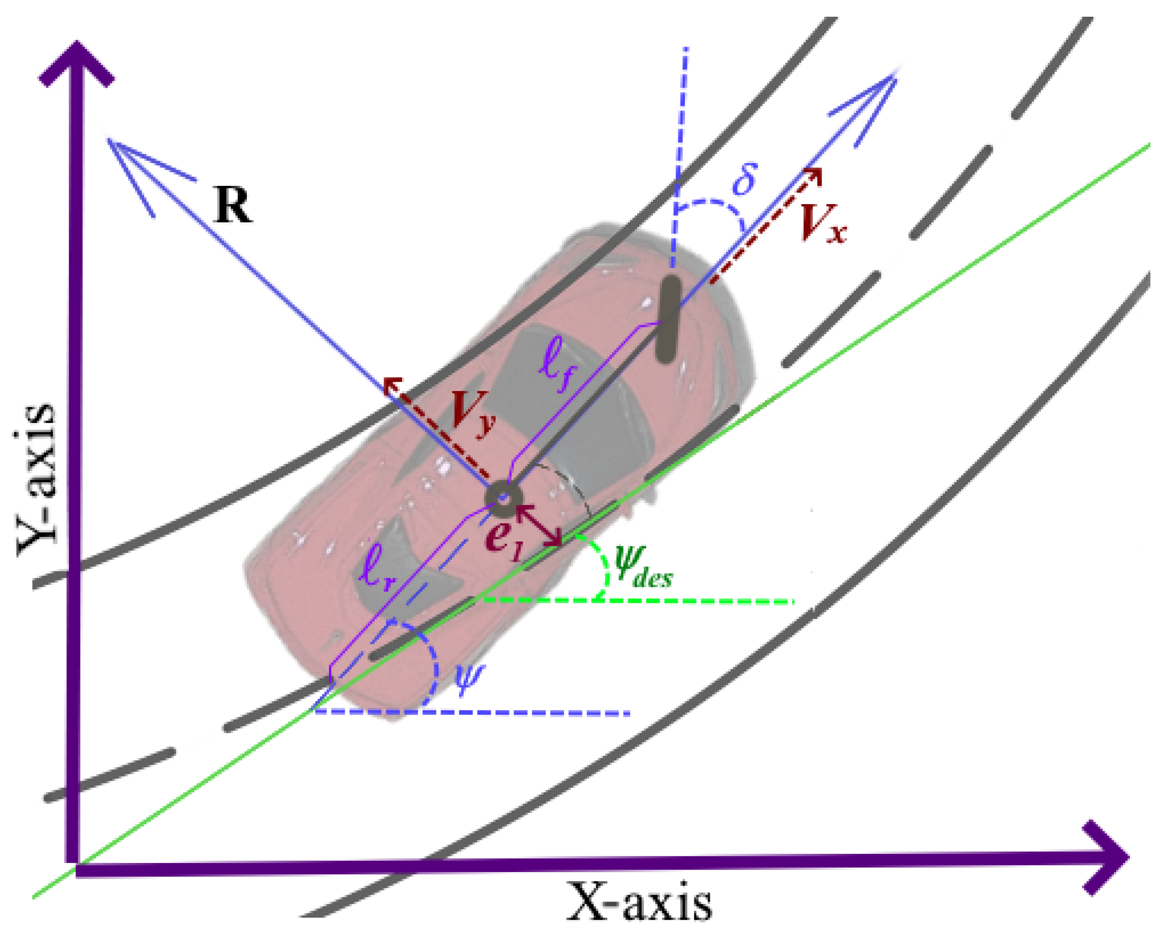
Most path-following controllers are designed based on a mathematical model of the vehicle. There are two common versions for a model of the vehicle: one related to the kinematics of the vehicle and the other oriented to describe its dynamics. The first is only concerned with expressing the geometry defined during the motion of the components of the vehicle without considering the forces and torques that generated this motion, and the latter includes these forces and torques in its equations. The proposed controller considers a dynamical model of the vehicle, in particular, the bicycle model [23]. It consists of a bar that connects the front and rear tires, as shown in Figure 2, and it has two degrees of freedom, which are the lateral position y and the orientation of the vehicle.

Figure 2.
Parameters and variables related to the lateral vehicle’s dynamics. R corresponds to instant trajectory radius.
In a path-following scenario, the controller’s objective is to force the pose (position and orientation) of the vehicle to track a desired pose defined by the path to follow. Let us consider an inertial coordinate system and a vehicle-fixed coordinate system , whose origin is located at the center of gravity (c.g.) of the vehicle and its axis is aligned with the longitudinal axis of the vehicle. Then, a reference path for the vehicle is expressed in the inertial coordinate system, which permits defining references for the coordinates of the vehicle and its orientation. It was assumed that these references are computed by an instrumentation system in a higher layer in the software/hardware architecture of the vehicle by means of data retrieved from sensors, such as cameras, an IMU, LIDAR, and ultrasonic sensors. Moreover, it was assumed that an external controller maintains the longitudinal velocity of the vehicle at a constant value.
Within this scenario, the lateral dynamics of the vehicle with respect to the inertial frame, according to [23], can be defined as
where , y is the distance from the c.g. of the vehicle to its center of rotation, is the heading angle (yaw angle) of the vehicle, is the front wheel steering angle, is its longitudinal velocity, and is the road bank angle. The parameters of the model are defined as , , , , , and , where and are the distances from the c.g. to the front and rear axes of the vehicle, and are the cornering stiffnesses of the rear and front wheels, is the momentum of inertia of the vehicle with respect to the normal axis of the reference system, m corresponds to the total mass of the vehicle, and g is the gravitational constant.
3. Overall Control Scheme
The proposed control scheme is shown in Figure 3, where , , and are the coordinates and orientation references for the vehicle, which correspond to the pose of the desired path. Furthermore, two control loops can be identified in the control scheme: the outer loop, which receives a reference for the pose of the vehicle and generates a reference for the steering angle , and the inner control loop, which receives the steering angle reference and generates the voltages that excite the actuator. The proposed controller considers a BLDC motor as the steering actuator of the vehicle. Hence, the input of the actuator is a three-phase voltage and its output is the current steering angle of the vehicle.
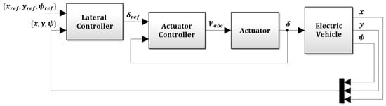
Figure 3.
Overall control scheme.
To design the global control scheme, two control algorithms must be designed: a lateral controller that receives a pose reference for the vehicle, which is defined by , , and , and generates a desired steering angle , and an actuator controller that receives and generates the input voltage for the BLDC motor of the steering system. The design of these controllers is given in the rest of this section.
3.1. Lateral Sliding Mode Controller
As mentioned before, the lateral controller receives the references , , and from the instrumentation sub-system of the vehicle. In addition, it also provides the current X- and Y-coordinates of the vehicle and its current orientation . From these values, it is possible to define the error variables , which is the distance between the vehicle’s c.g. and the center line of the road, and . Then, an error variables vector is established, as depicted in Figure 2. Hence, using (1), the error variables dynamics yields the following:
with
, , , and . According to this, the lateral controller objective is to design a control signal that stabilizes the system (2), i.e., the error variables and converge to zero in finite time. The controller design procedure, which is based on [24], and the closed loop stability analysis are stated in the following theorem.
Theorem 1.
Consider the sliding mode control law
where , , , , and the following conditions are fulfilled
Moreover, if , then the origin of the closed loop system is a globally asymptotically stable equilibrium point.
Proof.
First, a similarity transformation is defined as
where , which converts the system (2) into
with , , , , and . This transformation permits simplifying the designing procedure of the control law. Also, by means of (2), (4), and (6), a bound for can be obtained in the form
which represents an important definition, as it allows for establishing the values of the control gains that fulfill the control objective, as seen below. Then, a sliding surface is defined via a linear combination of the original error variables and, consequently, a linear combination of the transformed coordinates of the form
and, using (2) and (3), its derivative yields , which ensures the sliding mode occurrence in finite time as . During the sliding motion, we have , and from (9), we obtain
Now, by means of (7) and (10), a reduced system is obtained as follows:
with . Then, using the value of defined in the conditions of the theorem, the eigenvalues of the reduced system results in , and considering , , and , the reduced system corresponds to a globally exponentially asymptotically stable dynamical system. Now, let us define a candidate Lyapunov function for system (11) as , whose derivative takes the form of
Therefore, the trajectories of system (11) converge to a vicinity of its origin bounded by . From (6), we have that , which, using (8), (10), and , turns into
Finally, it is straightforward to demonstrate that if , the previous inequality reduces to . □
The lateral control law defined by the previous theorem represents a reference for the actuator controller of the vehicle, as shown in the following section.
3.2. Actuator Controller
A brushless direct current (BLDC) motor was used as the steering actuator of the vehicle. Its dynamics ([25,26,27,28]) are described by the following equation
where is the three-phase input voltage, is the three-phase current vector, is the three-phase back-electromagnetic force, is the electrical rotor angle, is the angular velocity of the rotor in rad/s, P is the number of poles, R is the armature resistance, L is the self-inductance, M is the mutual inductance of the motor, b is the viscous friction coefficient of the motor’s axle, is the generated electrical torque, and is the load torque experienced by the motor. It is important to note that corresponds to the steering angle of the vehicle, which represents the input signal for the vehicle’s lateral dynamics system. In addition, these equations are valid under the following assumptions:
- The motor is not saturated and should be operated with the rated current.
- The resistances of the three stator phase windings are equal.
- The self-inductance and mutual inductance of the motor are constant.
- The switching of the semiconductor devices is ideal.
The BLDC motor equations in (13) are expressed in the a-b-c coordinates, which means that the voltage and currents signals of the motor are defined with respect to a static three-phase reference frame whose basic vectors are shifted in phase rad with respect to each other as follows:
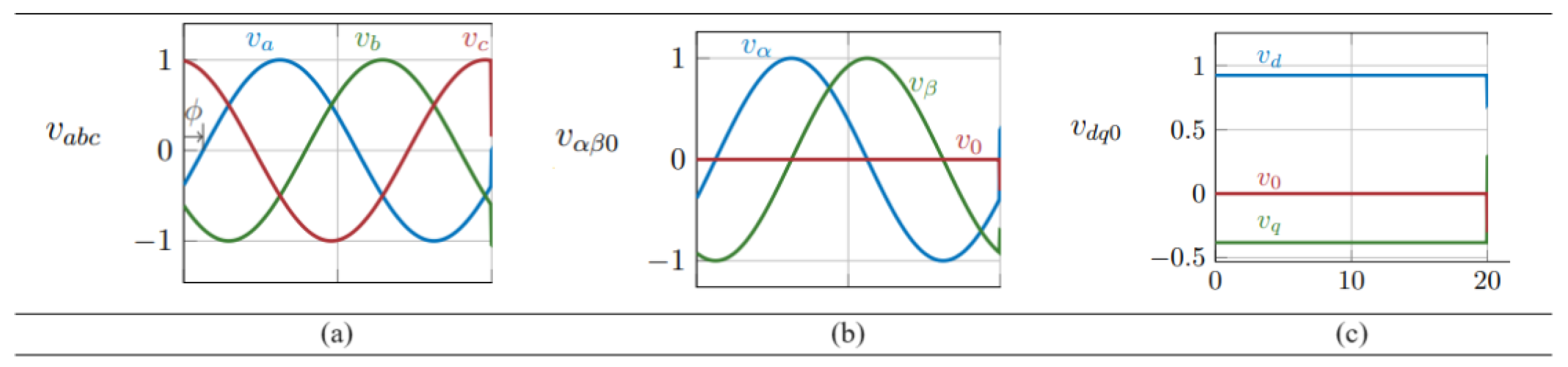
However, designing a control algorithm in this reference frame is complicated. Hence, the Park–Clarke transformation, also known as the direct–quadrature–zero transformation, is used to express the model of the motor in d-q-0 coordinates, which simplify the control design procedure. This is because it permits expressing the signals of the motor as constant values instead of sinusoidal waveforms, as the reference frame is attached to the rotor of the motor. The d component of this reference represents the magnetic flux and the q component represents the torque produced by the currents of the motor. As its name suggests, it is composed of two singular transformations: the Park and Clarke transformations. The former results in --0 coordinates that correspond to a static frame aligned to one of the original basic vectors, which reduces the significant components to only two [25]. This process is depicted in Figure 4.
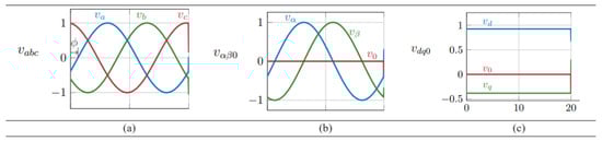
Figure 4.
Voltage signals expressed in the three reference frames: (a) , (b) , and (c) .
The Park–Clarke transform and inverse are defined as
and
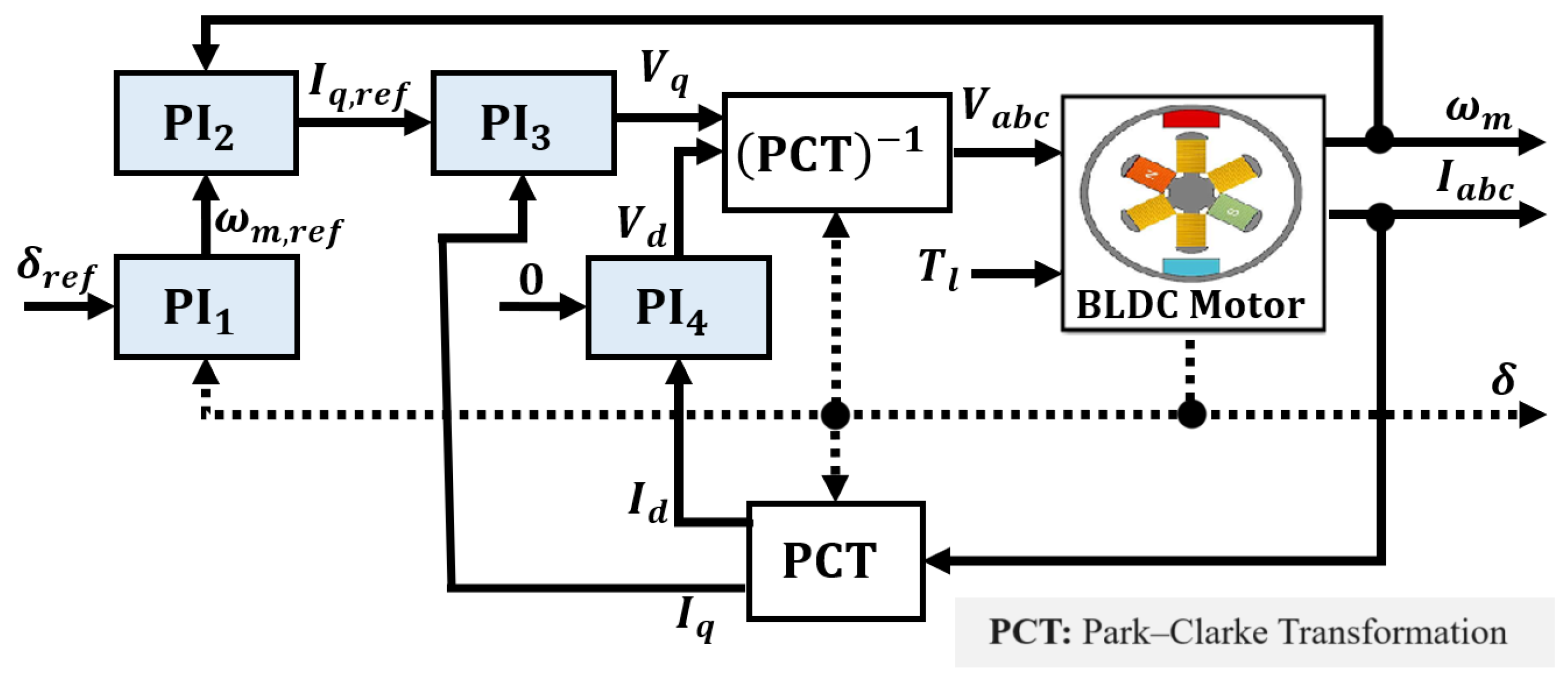
The primary goal of FOC is to independently control the torque and flux in the motor, allowing for better performance in terms of the speed control, torque response, and efficiency. To this end, the control strategy consists of the following stages: first, the controller receives the reference for the angular position of the axle ; then, a PI controller defines a variable error between this reference and the current angular position of the motor and generates a reference for the angular velocity of the motor ; after this, the second PI controller defines an error with the current angular velocity of the motor and generates a reference for the quadrature current of the motor ; next, the third PI controller uses the actual quadrature current of the motor to generate a desired quadrature voltage to be applied to the motor and, at the same time, the fourth PI controller defines a desired direct voltage of the motor in order for the direct current to remain zero; finally, via the Park–Clarke transform, the voltages are converted to in order to be applied to the BLDC motor. It is worth noting that the Park–Clarke transform and its inverse are necessary to transform the voltages and currents of the motor from the a-b-c coordinates to the d-q-0 coordinates and vice versa. This process is depicted in Figure 5, which shows a classic FOC scheme with an additional proportional–integral (PI) controller for the angular position of the motor. In the figure, the block corresponds to the Park–Clarke transformation and the block to its inverse.
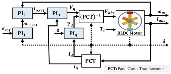
Figure 5.
BLDC motor’s angular position control scheme.
Overall, the control strategy is composed of four PI controllers and their corresponding proportional and integral control gains. The first is used to control the angular position of the motor with gains ; the second is for controlling the angular velocity with gains ; and the rest control and with gains and , correspondingly.
The tuning process for all the PID controllers was based on a combination of the PID Tuning toolbox in Matlab/Simulink and an additional fine-tuning stage, which was done manually. The tuning process order was as follows: first, and were tuned and the voltages and were stabilized; then, was tuned and the angular speed was controlled; finally, , which controls the angular position of the motor, was tuned. For more information regarding the field-oriented control and the reference frame, please refer to [25].
4. Simulation Results
The parameters used for the simulation results presented in this section are defined in Table 1 and the gains of the overall control law are shown in Table 2. It is worth noting that the control gains of the lateral sliding mode controller were tuned according to the necessary stability conditions established by Theorem 1, and the gains of the actuator’s controller were tuned heuristically. Furthermore, if the reader wishes to reproduce these results, the Simulink model can be downloaded from [29] or [30], and the configuration of the Simulink model is described in detail in Appendix A.

Table 1.
Parameters of the vehicle and the actuator.
Table 2.
Control gains for lateral and actuator controllers.
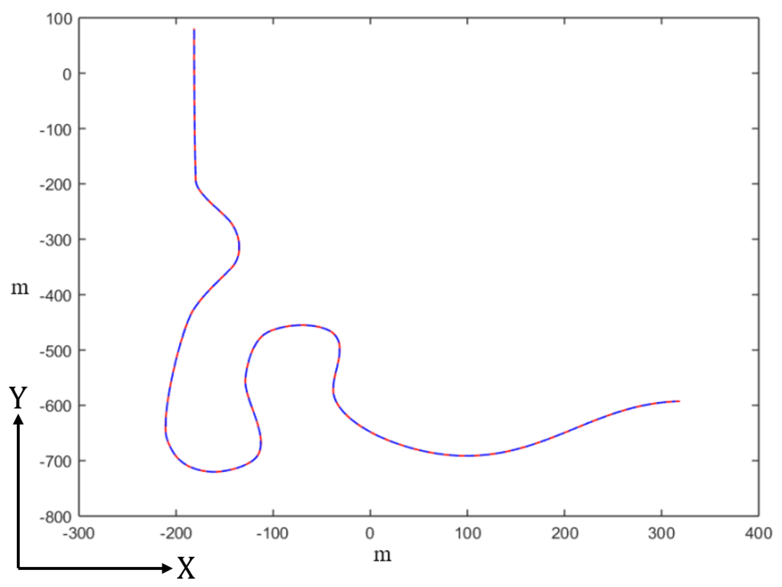
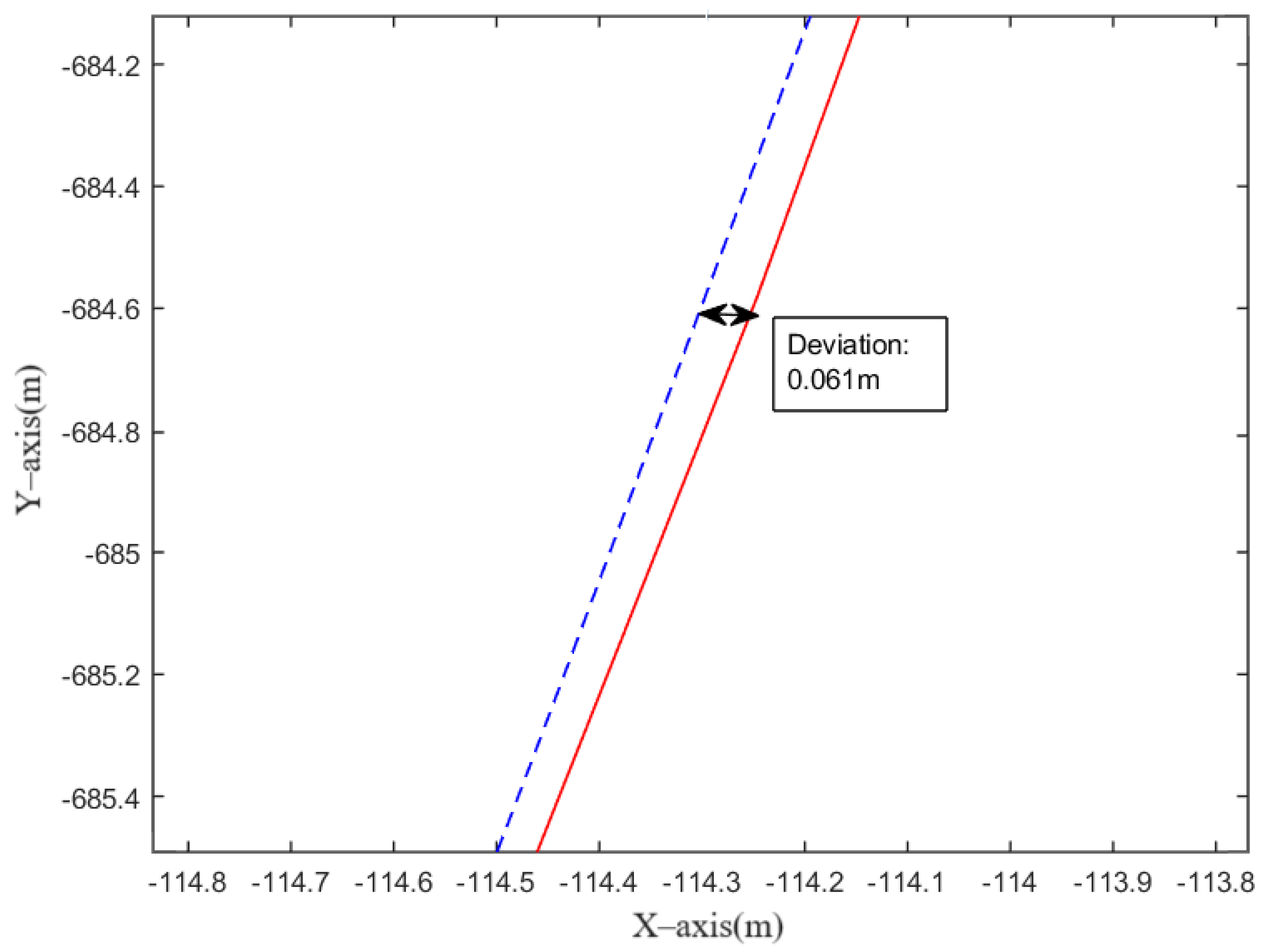
The path-following behavior of the proposed control scheme in the coordinate plane is shown in Figure 6 for the whole experiment, where the dashed blue line corresponds to the current position of the vehicle and the solid red line represents the reference trajectory. It can be noted that the performance of the closed loop system was satisfactory, as the control objective was achieved, even when considering a constant longitudinal velocity of 22 m/s (79.2 km/h) and a constant road bank angle of 0.174533 rad (10°). The experiments were carried out with different values of longitudinal velocity and road bank angle; however, only the results obtained with the extreme values are reported, as we assumed that these better demonstrated the capabilities of the proposed control scheme. This can also be appreciated in Figure 7, where a close-up of the previous figure is presented, and the small difference between the reference path and the position of the vehicle is more visible.
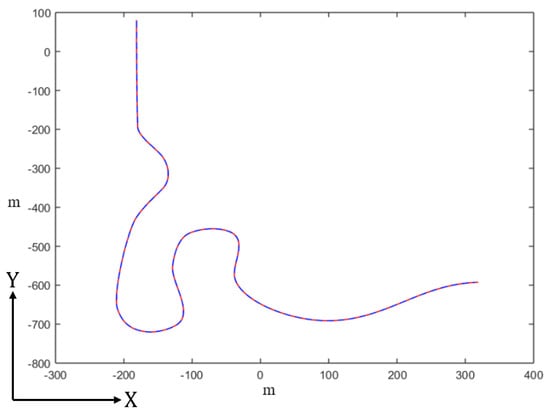
Figure 6.
Results of the path-following experiment, where the current path (dashed blue line) and the reference trajectory (solid red line) are depicted.
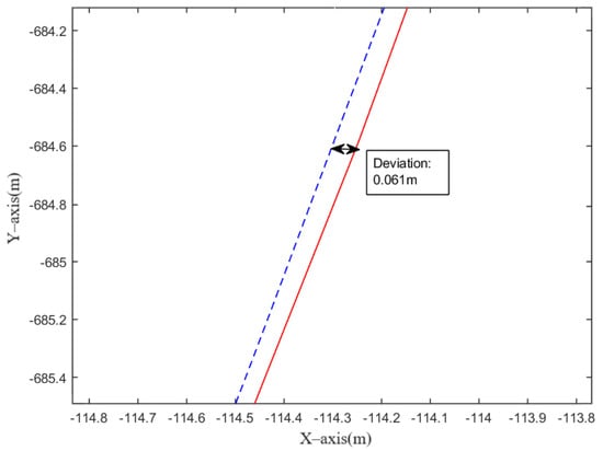
Figure 7.
Close-up of the path-following experiment depicted in Figure 6, where the tracking error can be appreciated.
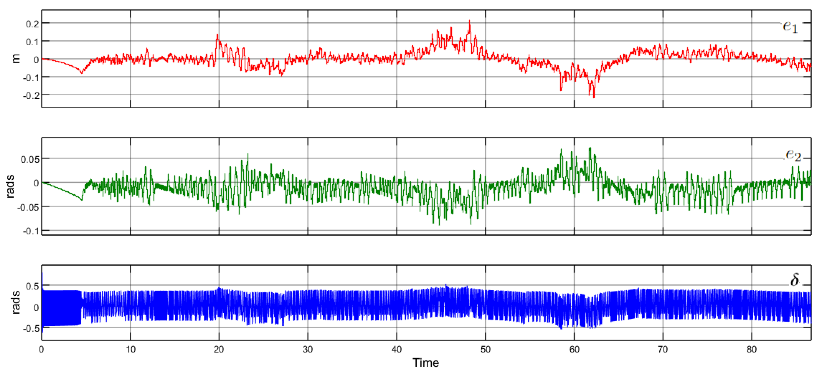
This path-following error is also depicted at the top of Figure 8, where its maximum value during the whole experiment was 0.21 m and its average value was 0.033 m. Moreover, the heading angle error variable is shown in the middle of the figure, where its maximum value was 0.09 rad and its average value was 0.019 rad. Also, the bottom of the figure depicts the steering angle of the vehicle, which had a maximum value of 0.25 rad (14.32°). It is important to emphasize that the bound of the resulting steering angle corresponds to the bound of the steering angle of a real automotive vehicle. This will be crucial if a real-time implementation of the proposed controller is considered.
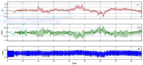
Figure 8.
Error variables (top) and (middle), and control signal (bottom) of the lateral controller of the vehicle during the experiment.
Figure 9 shows the states of the lateral dynamical model, which correspond to the distance to the path y, the heading angle of the vehicle , and their corresponding derivatives. In addition, Figure 10 depicts the actuator’s mechanical and electrical states.
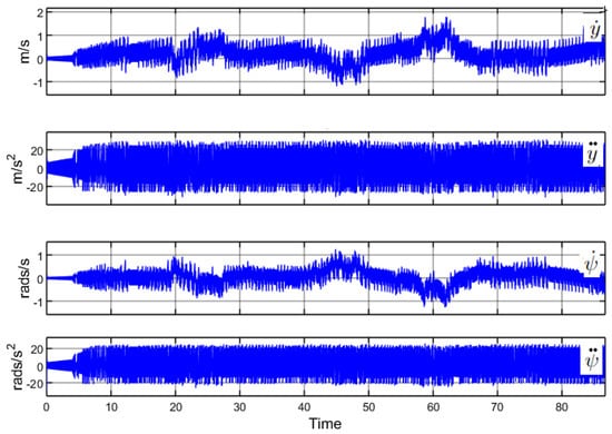
Figure 9.
States of the lateral dynamics of the vehicle.
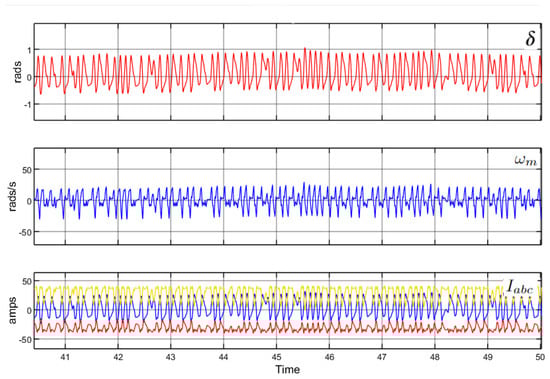
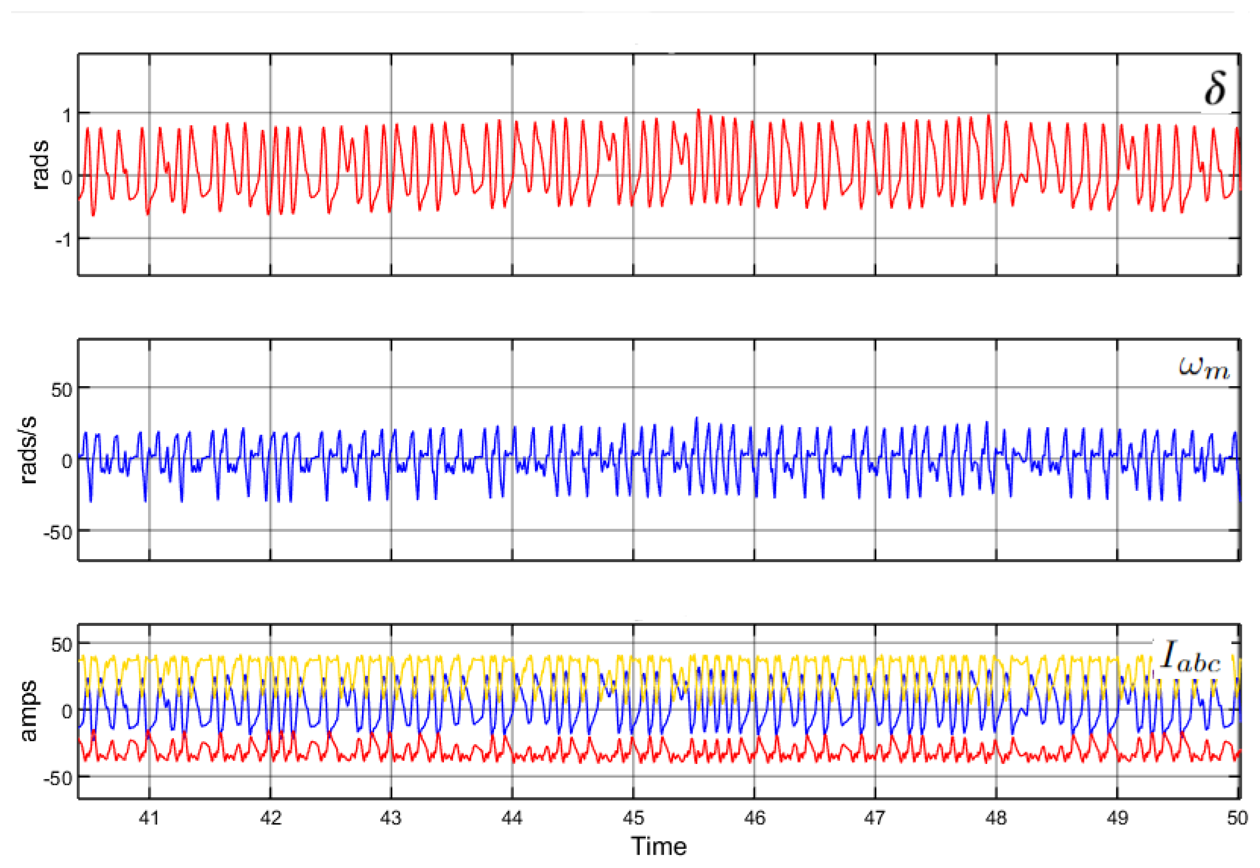
Figure 10.
BLDC internal states: (top), (center), and (bottom).
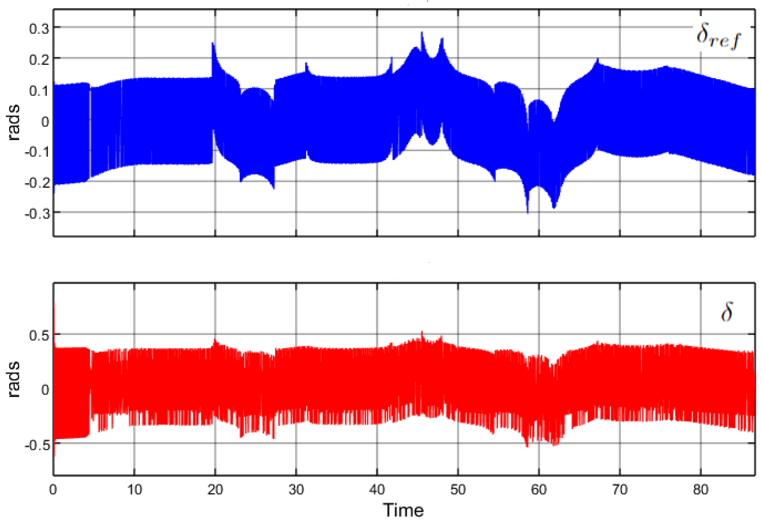
The performance of the actuator’s controller can be assessed by means of Figure 11, where the steering angle and its reference are shown. Also, this performance can be interpreted from Figure 12, where the error variables for the four internal PID controllers of the actuator are shown. It can be appreciated that the low-frequency steady state of the four error variables converged to the vicinity of zero, thus ensuring the fulfillment of the control objective.

Figure 11.
Steering angle and its reference during the experiment.
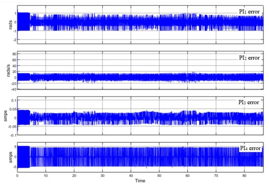
Figure 12.
Error variables of the 4 PI controllers in the BLDC control loop.
5. Discussion
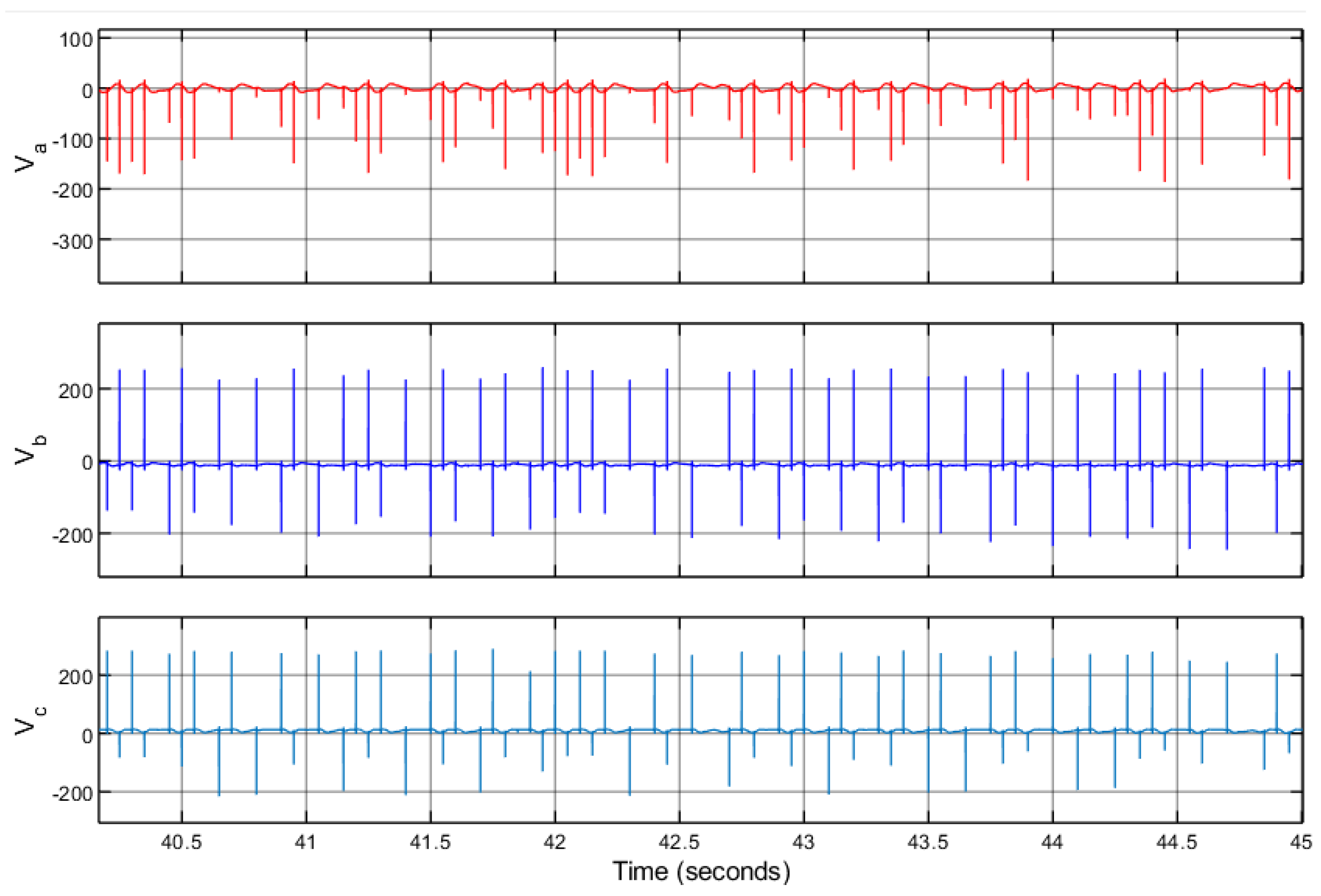
The simulation results presented in the previous section demonstrate that the designed control scheme achieved the path following of the proposed reference in a satisfactory manner. This is depicted in Figure 8, where a maximum lateral error of 0.2 m was presented during the experiment. It is worth noting that the experiment was carried out at a constant longitudinal speed of 80 km/h in comparison with [6], where the maximum test speed was 40 km/h. Moreover, a constant bank road angle was considered during the whole experiment, which represents another factor to be counteracted by the control law. Additionally, the actuator dynamics were considered for the simulations, which represent a more realistic implementation of the controller, as the generated control signals correspond to the voltage input of the electric actuator, which was assumed to be a BLDC electric motor according to most of the current commercial electric vehicles. To obtain this response, the actuator’s current demand was up to 50 A in its peak value, which fell within the limits of most of the available drivers for this type of motor. On the other hand, and due to the application of standard sliding modes, the control signals were characterized by the presence of high-frequency components, as shown in Figure 13 and Figure 14. Although this chattering effect was less visible in the mechanical variables of the vehicle, this is still an undesired feature of the proposed controller, as it reduces the life cycle of the actuators. Despite this, the overall effectiveness of the control scheme was demonstrated by means of the presented simulation results.
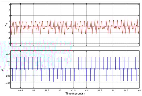
Figure 13.
Input voltages for the BLDC motor in the reference frame.
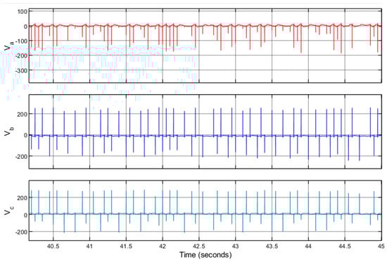
Figure 14.
Input voltages for the BLDC motor in the reference frame.
6. Conclusions and Future Work
A control scheme based on sliding modes for an electric vehicle following a path is presented. In addition, the control schemes considered a PI-based FOC (field-oriented control) for the steering actuator, which was assumed to be a BLDC motor. The general performance of the proposal was satisfactory, as the control objective was fulfilled despite considerations such as a constant 80 km/h longitudinal velocity and a constant road bank angle. In comparison with other works, the inclusion of the actuator dynamics represents a more realistic design for the control signal, which corresponds to the voltage of the electric actuator. Despite the presence of high-frequency components in the resulting control signal, the effectiveness of the overall control algorithm was demonstrated, as low bounds for the lateral error and yaw angle error variables were attained.
The next steps for this work will be oriented to the inclusion of high-order sliding modes (HOSMs) to the controller design to avoid the presence of high-frequency components in the control signal. Moreover, the implementation of the designed control scheme on simulators, such as CARLA [31] or CarSim [32], to enhance the complexity and realism of the experimental scenarios and to include the effect of sensors and signal conditioning stages in the performance of the controller can be included. Another improvement that will be implemented in future stages of the project is to consider the dynamic double-track model of the vehicle during the controller design process. The motivation is to increase the accuracy of the model, especially when the vehicle is operating at high speed and lateral tire slip is present during the experiments.
Author Contributions
Conceptualization, L.E.G.-J., L.A.T.-R. and R.R.-C.; methodology, L.E.G.-J. and L.A.T.-R.; software, L.A.T.-R.; validation, L.E.G.-J., L.A.T.-R. and R.R.-C.; formal analysis, L.E.G.-J. and R.R.-C.; investigation, L.E.G.-J., L.A.T.-R. and R.R.-C.; resources, L.E.G.-J., L.A.T.-R. and R.R.-C.; data curation, L.E.G.-J. and L.A.T.-R.; writing—original draft preparation, L.E.G.-J., L.A.T.-R. and R.R.-C.; writing—review and editing, L.E.G.-J., L.A.T.-R. and R.R.-C.; visualization, L.A.T.-R. and L.E.G.-J.; supervision, L.E.G.-J. and R.R.-C.; project administration, L.E.G.-J. and R.R.-C. All authors read and agreed to the published version of the manuscript.
Funding
This research was funded by Mexican National Council of Humanities, Science and Technology (CONAHCyT) by the scholarships 453637, 172488, and 40326.
Institutional Review Board Statement
Not applicable.
Informed Consent Statement
Not applicable.
Data Availability Statement
The dynamical model of the vehicle and the proposed controller can be found in [29].
Conflicts of Interest
The authors declare no conflicts of interest.
Abbreviations
The following abbreviations are used in this manuscript:
| BLDC | Brushless direct current motor |
| FOC | Field-oriented control |
| SVPWM | Space vector pulse-width modulation |
| PI | Proportional–integral control |
| MPC | Model predictive control |
| IMU | Inertial measurement unit |
| LIDAR | Light detection and ranging |
| SMC | Sliding mode control |
| SAE | Society of Automotive Engineers |
| HOSM | High-order sliding mode |
| LKAS | Lane-keeping assist system |
| LDA | Lane departure avoidance |
| ELKS | Emergency lane-keeping system |
Appendix A. Configuration of the Closed-Loop System in Simulink
This section is intended to give specific hints that were used to obtain the corresponding reported results in case the reader wishes to simulate the Simulink dynamical model defined in this work [29,30]. The main blocks comprising the Simulink model are depicted in Figure A1.
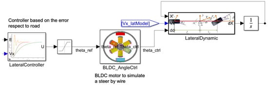
Figure A1.
Block structure for the lateral controller in the Simulink model.
Figure A1.
Block structure for the lateral controller in the Simulink model.
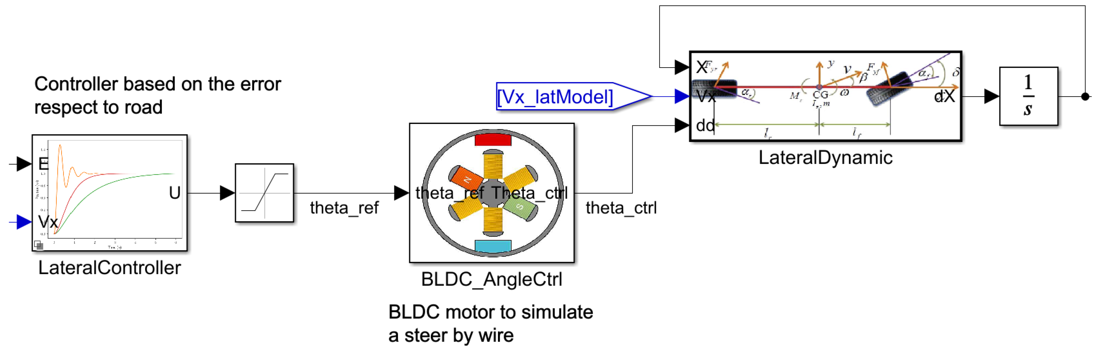
First, it is required to set up the model to make it easier to run. The model consists of lateral and longitudinal dynamics. Since the longitudinal dynamics are not required, the upper section can be commented out; this will result in a lighter model and a reduced simulation period. Since the longitudinal dynamics are removed, the longitudinal velocity needs to be added manually. For this, the “Signal Generator” block, which is already contained in the model, is connected to the label “Vx_latModel”. You can manually specify the velocity profile you wish for the experiment. In our case, this was set up to be 22 m/s (80 km/h approx).
In the left, the “LateralController” block is a variant block. Choose the variant “SMC Conventional V2”, which is the implementation of the proposed controller. In the middle, the block “Actuator” is a variant block where you can choose between “BLDC”, “generic transfer function”, or “No Actuator” as the corresponding model of the actuator. To replicate the reported simulations, the option “BLDC”, which converts the model into a stiff system, must be selected. If the model is executed, the accuracy of the simulations will be severely decreased. To fix this issue, the model settings must be redefined. In particular, the ODE solver must be set to a fixed step size solver with a sample time of s. The block to the right is the implementation of the lateral dynamics. This is a variant block too, and hence, it must be configured to “Not simplified model”. This ends the configuration process of the model.
References
- Alcala, E.; Sellart, L.; Puig, V.; Quevedo, J.; Saludes, J.; Vázquez, D.; López, A. Comparison of two non-linear model-based control strategies for autonomous vehicles. In Proceedings of the 24th Mediterranean Conference on Control and Automation (MED), Athens, Greece, 21–24 June 2016; pp. 846–851. [Google Scholar]
- Ritzer, P.; Winter, C.; Brembeck, J. Advanced path following control of an overactuated robotic vehicle. In Proceedings of the 2015 IEEE Intelligent Vehicles Symposium (IV), Seoul, Republic of Korea, 28–30 June 2015; pp. 1120–1125. [Google Scholar]
- Yuan, X.; Huang, G.; Shi, K. Improved Adaptive Path Following Control System for Autonomous Vehicle in Different Velocities. IEEE Trans. Intel. Transp. Syst. 2020, 21, 3247–3256. [Google Scholar] [CrossRef]
- Fernandez, B.; Herrera, P.; Cerrada, J. A Simplified Optimal Path Following Controller for an Agricultural Skid-Steering Robot. IEEE Access 2019, 7, 95932–95940. [Google Scholar] [CrossRef]
- Hossain, T.; Habibullah, H.; Islam, R. Steering and Speed Control System Design for Autonomous Vehicles by Developing an Optimal Hybrid Controller to Track Reference Trajectory. Machines 2022, 10, 420. [Google Scholar] [CrossRef]
- Ritschel, R.; Schrödel, F.; Hädrich, J.; Jäkel, J. Nonlinear Model Predictive Path-Following Control for Highly Automated Driving. IFAC-PapersOnLine 2019, 52, 350–355. [Google Scholar] [CrossRef]
- Vu, T.M.; Moezzi, R.; Cyrus, J.; Hlava, J. Model Predictive Control for Autonomous Driving Vehicles. Electronics 2021, 10, 2593. [Google Scholar] [CrossRef]
- Ultsch, J.; Mirwald, J.; Brembeck, J.; De Castro, R. Reinforcement Learning-based Path Following Control for a Vehicle with Variable Delay in the Drivetrain. In Proceedings of the 2020 IEEE Intelligent Vehicles Symposium (IV), Las Vegas, NV, USA, 19–30 October 2020; pp. 532–539. [Google Scholar]
- Guo, N.; Zhang, X.; Zou, Y.; Lenzo, B.; Zhang, T. A Computationally Efficient Path-Following Control Strategy of Autonomous Electric Vehicles with Yaw Motion Stabilization. IEEE Trans. Transp. Electrif. 2020, 6, 2. [Google Scholar] [CrossRef]
- Liang, J.; Tian, Q.; Feng, J.; Pi, D.; Yin, G. A polytopic model-based robust predictive control scheme for path tracking of autonomous vehicles. IEEE Trans. Intell. Veh. 2023, 1–11. [Google Scholar] [CrossRef]
- Hu, C.; Wang, R.; Yan, F. Integral Sliding Mode-Based Composite Nonlinear Feedback Control for Path Following of Four-Wheel Independently Actuated Autonomous Vehicles. IEEE Trans. Transp. Electrif. 2016, 2, 2. [Google Scholar] [CrossRef]
- De Castro, R.; Tanelli, M.; Esteves, A.R.; Savaresi, S.M. Minimum-Time Path-Following for Highly Redundant Electric Vehicles. IEEE Trans. Control Syst. Technol. 2016, 24, 2. [Google Scholar] [CrossRef]
- Utkin, V.; Guldner, J.; Shi, J. Sliding Mode Control in Electro-Mechanical Systems; CRC Press: Boca Raton, FL, USA, 2009. [Google Scholar]
- Solea, R.; Nunes, U. Trajectory planning and sliding-mode control based trajectory-tracking for cybercars. Integr. Comput.-Aided Eng. 2007, 14, 33–47. [Google Scholar] [CrossRef]
- Oh, K.; Seo, J. Development of a Sliding-Mode-Control-Based Path-Tracking Algorithm with Model-Free Adaptive Feedback Action for Autonomous Vehicles. Sensors 2023, 23, 405. [Google Scholar] [CrossRef]
- Kim, H.; Kee, S.-C. Neural Network Approach Super-Twisting Sliding Mode Control for Path-Tracking of Autonomous Vehicles. Electronics 2023, 12, 3635. [Google Scholar] [CrossRef]
- Wu, Y.; Wang, L.; Li, F.; Zhang, J. Robust sliding mode prediction path tracking control for intelligent vehicle. Proc. Inst. Mech. Eng. Part I J. Syst. Control Eng. 2022, 236, 1607–1617. [Google Scholar] [CrossRef]
- Wang, C.; He, R.; Xia, Q. Path following control for 4WID-EV based on extended state observer and sliding mode control considering yaw stability. Adv. Mech. Eng. 2023, 15. [Google Scholar] [CrossRef]
- Ljungqvist, O.; Evestedt, N.; Axehill, D.; Cirillo, M.; Pettersson, H. A path planning and path-following control framework for a general 2-trailer with a car-like tractor. J. Field Robot. 2019, 36, 1345–1377. [Google Scholar] [CrossRef]
- Woo, J.; Yu, C.; Kim, N. Deep reinforcement learning-based controller for path following of an unmanned surface vehicle. Ocean Eng. 2019, 183, 155–166. [Google Scholar] [CrossRef]
- Maurya, P.; Morishita, H.M.; Pascoal, A.; Aguiar, A.P. A Path-Following Controller for Marine Vehicles Using a Two-Scale Inner-Outer Loop Approach. Sensors 2022, 22, 4293. [Google Scholar] [CrossRef] [PubMed]
- Paden, B.; Cap, M.; Yong, S.; Yershov, D.; Frazzoli, E.; Vázquez, D. A Survey of Motion Planning and Control Techniques for Self-Driving Urban Vehicles. IEEE Trans. Intel. Veh. 2016, 1, 33–35. [Google Scholar] [CrossRef]
- Rajamani, R. Vehicle Dynamics and Control; Springer Science & Business Media: New York, NY, USA, 2011. [Google Scholar]
- Shtessel, Y.; Edwards, C.; Fridman, L.; Levant, A. Sliding Mode Control and Observation; Springer: New York, NY, USA, 2014. [Google Scholar]
- Bose, B.K. Modern Power Electronics & AC Drives; Prentice Hall: Englewood Cliffs, NJ, USA, 2002. [Google Scholar]
- Bolton, W.C. Mechatronics: Electronic Control Systems in Mechanical and Electrical Engineering; Pearson Education: Harlow, UK, 2018. [Google Scholar]
- Mondal, S.; Mitra, A.; Chattopadhyay, M. Mathematical modeling and simulation of brushless DC motor with ideal back emf for a precision speed control. In Proceedings of the 2015 IEEE International Conference on Electrical, Computer and Communication Technologies (ICECCT), Coimbatore, India, 5–7 March 2015; pp. 1–5. [Google Scholar]
- Pillay, P.; Krishnan, R. Modeling, simulation, and analysis of permanent-magnet motor drives. IEEE Trans. Ind. App. 1989, 25, 265–273. [Google Scholar] [CrossRef]
- Vehicle Dynamics and Controller Simulink Model. Available online: https://github.com/L-Arturo-Torres-Romero/VehicleModel/tree/master/VehicleModel (accessed on 24 October 2023).
- Torres-Romero, L. L-Arturo-Torres-Romero/VehicleModel: Conventional SMC for Lateral Dynamic 2; Zenodo: Geneva, Switzerland, 2024. [Google Scholar] [CrossRef]
- CARLA: Open-Source Simulator for Autonomous Driving Research. Available online: http://carla.org (accessed on 10 November 2023).
- CarSim: Mechanical Simulation. Available online: https://www.carsim.com/ (accessed on 27 November 2023).


Disclaimer/Publisher’s Note: The statements, opinions and data contained in all publications are solely those of the individual author(s) and contributor(s) and not of MDPI and/or the editor(s). MDPI and/or the editor(s) disclaim responsibility for any injury to people or property resulting from any ideas, methods, instructions or products referred to in the content. |
© 2024 by the authors. Licensee MDPI, Basel, Switzerland. This article is an open access article distributed under the terms and conditions of the Creative Commons Attribution (CC BY) license (https://creativecommons.org/licenses/by/4.0/).