Thermomechanical Rotor Fatigue of an Interior Permanent Magnet Synchronous Motor

Abstract

Interior permanent magnet synchronous motors (IPMSMs) are extensively used as traction motors today because of their exceptional torque, power density, and wide, constant power operating range. Under real-world usage, an IPMSM rotor undergoes varying electromagnetic, thermal, and mechanical loads. Under such conditions, fatigue life-based design criteria should be used over stress-based design criteria to ensure the structural integrity of the rotor. Moreover, the driving dynamics can change the rotor temperature continuously, which affects the electromagnetic, mechanical, and fatigue properties of the rotor material. This paper proposes a robust thermomechanical rotor fatigue simulation workflow considering significant loads acting on an IPMSM rotor and the temperature variation throughout a drive cycle. It discusses an accelerated fatigue life estimation approach based on the peak valley extraction method to reduce the simulation time significantly for the stress and fatigue analysis. Then, it presents a method for a stress-life curve generation for variable loading. It also presents a sensitivity study with a median S-N curve, and a 90% reliability and 95% confidence (R90C95) S-N curve.

1. Introduction

The rising popularity of electric vehicles (EVs) has compelled automotive manufacturers to seek traction motors that offer remarkable torque capabilities, high power density, and a broad operational speed range. Interior permanent magnet synchronous motors (IPMSMs) are among the most appealing choices, as they align with these crucial traction motor requirements [1,2]. A higher rotor speed improves the power density of the motor [3]. However, a higher motor speed can also have a damaging effect on the IPMSM rotor because the centrifugal load is quadratically proportional to the speed. An IPMSM usually requires a thinner rotor bridge to improve torque performance, but it leads to an increase in stress at the rotor bridges [4]. The rotor is also affected by electromagnetic, thermal, and other mechanical loads. Hence, evaluating the rotor for all loads is critical to ensure its structural integrity.

Furthermore, the rotor goes through fluctuating temperatures and speeds during drive cycles. The fluctuating temperature leads to changes in electrical, electromagnetic, and mechanical properties of the materials in an IPMSM. Fluctuating speeds lead to a change in the mean and amplitude load, which should also be accounted for to ensure the structural integrity of the rotor. Hence, it is critical to calculate the fatigue life of the rotor, taking into account the fluctuating speed and temperature.

Thermal management of an IPMSM motor is critical, as it has an adverse effect on the motor performance. As the temperature increases, the flux density of rare earth magnets decreases reversibly and, beyond a specific temperature, it may be demagnetized irreversibly [5]. Moreover, higher temperature leads to higher copper losses and may reduce the life expectancy of coils [6,7]. Therefore, ensuring a proper cooling mechanism for the IPMSM motor is critical to its performance. Electromagnetic–thermal coupled analysis has previously been used to design the motors [8,9]. A lumped parameter thermal network (LPTN) approach has been used to evaluate the thermal performance of a motor for a drive cycle because it is computationally economical.

Rotor stress due to the electromagnetic, thermal, and centrifugal load calculated through finite element simulations has been compared in a few publications in the literature. The rotor stress due to thermal load and centrifugal load was much higher than stress due to electromagnetic load in [10], whereas the rotor stress due to centrifugal load was significantly higher than the stress due to thermal and electromagnetic load in [11]. A rotor fatigue analysis has been carried out for a drive cycle considering only the centrifugal load in [12,13]. The rotor stress considering the thermal and centrifugal load was studied for a drive cycle, and the fatigue analysis was carried out using analytical calculations in [14]. The fatigue analysis for drive cycles requires stress results for all time steps, which could be computationally expensive. An equivalent damage approach has been used to create block cycles instead of drive cycles in [11,15]. The peak–valley extraction method has been discussed to remove the non-damaging cycles from a drive cycle in [16].

A strain-life (E-N) approach is preferred over a stress-life (S-N) approach if the stress exceeds yield strength. Rotor laminations are made of thin electrical steel sheets, and it is usually challenging to extract their E-N fatigue material properties. In [14,17], S-N properties have been extracted for a positive stress ratio and used for fatigue life estimation. The stress ratio here refers to the ratio of the maximum and minimum load used for fatigue testing of specimens to extract fatigue material properties. The fatigue life was affected by multiple factors, such as surface roughness, mean stress effect, and fatigue life scatter, in [18,19,20,21]. The effect of surface roughness on the fatigue life of electrical steel has been studied in [11,17]. The surface roughness due to various cutting methods of electrical steel was discussed in [22].

This paper proposes a thermomechanical fatigue workflow for an IPMSM rotor. The rotor stress due to the electromagnetic, thermal, and mechanical load is presented. A drive cycle is defined for the rotor fatigue analysis. The thermal analysis of the motor is carried out, the cooling parameters are determined to meet the magnet and coil maximum temperature limit, and the rotor temperature profile for the drive cycle is calculated. The peak–valley approach is utilized to compress the drive cycle and eliminate the non-damaging cycles. The fatigue life is then calculated using the compressed drive cycle and the rotor temperature profile.

2. Rotor Stress Due to Electromagnetic, Thermal, and Mechanical Loads

In an IPMSM, electromagnetic forces are generated as a result of an electromechanical energy conversion. Since the rotor laminations are made of electrical steel, these forces lead to stress on the rotor lamination. The electromagnetic forces have a tangential component leading to torque and a radial component leading mainly to stator vibrations. Furthermore, operational conditions induce copper, core, and mechanical losses, which cause the rotor temperature to rise. This rise in temperature, in turn, causes thermal expansion, subjecting the rotor to the thermal loading. Also, the IPMSM rotor undergoes centrifugal load because of its rotation. Stress induced due to the centrifugal load is quadratically proportional to speed. Notably, an interference fit between the shaft and the rotor also contributes to rotor stress.

2.1. Loads and Boundary Conditions

A finite element analysis is carried out on an eight-pole IPMSM rotor to analyze the rotor stress due to the electromagnetic, thermal, and mechanical load.

Table 1. Interior permanent magnet synchronous motor parameters.

Parameters	Values	Units
Base speed	3750	RPM
Nominal DC voltage	350	V
Maximum rotor speed	18,000	RPM
Peak/continuous torque	438/193	Nm
Stator outer diameter	220	mm
Rotor outer diameter	150	mm
Axial length	150	mm
Number of poles	8	-
Rotor and stator lamination material	20SW1200	-
Magnet material	G48UH	-
Shaft material	Hot rolled steel	-

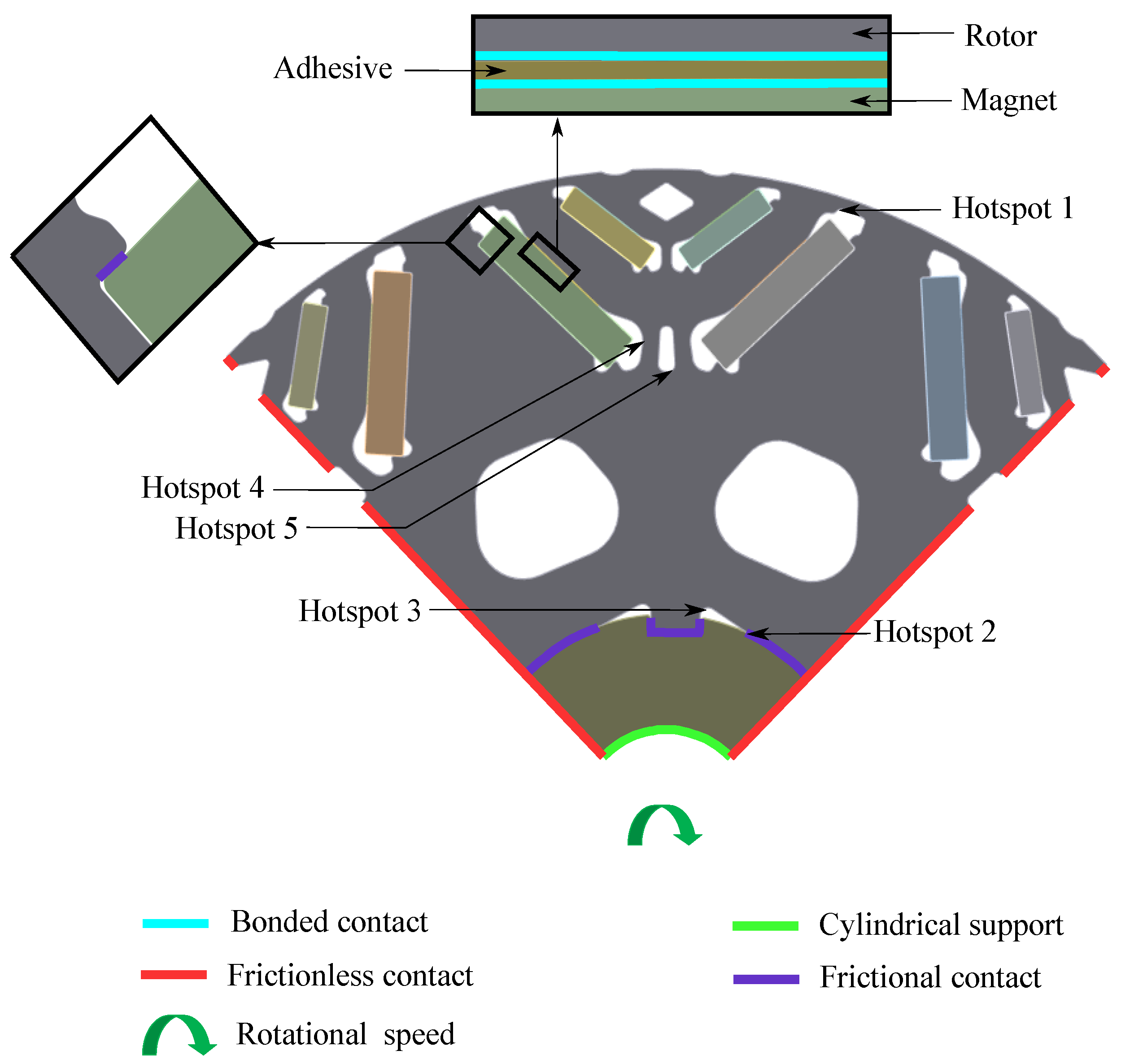
details the parameters of the IPMSM. The electromagnetic characteristics of this motor were presented in [23]. A rotor lamination quarter-symmetric model is considered for the rotor stress calculation because the rotor has four keys, as shown in Figure 1. It also shows loads and boundary conditions for the rotor stress analysis. During the rotor assembly, adhesive is applied at the bottom and the upper edge of the magnet. However, during real-world application, the lower adhesive layer deteriorates over time, so it has not been considered for the simulation. The adhesive is modeled between the rotor and the magnet’s upper surface using bonded contact to introduce realistic stiffness to the joint. A frictional contact is defined between the rotor and outer edges of the magnets to avoid singularity errors during the simulation. A frictional contact is applied between the shaft and the rotor. A frictional-less contact is defined on the symmetric boundary edges of the rotor and shaft and on one face of the rotor assembly, considering it is the endmost lamination of the rotor stack. A cylindrical support is considered on the inner diameter of the shaft with a free radial degree of freedom.

Electromagnetic forces are calculated in the Ansys Maxwell software for peak torque condition and applied to the rotor as body force density in the Ansys Mechanical software. The centrifugal load is applied considering the maximum rotational speed about the central axis of the rotor assembly. The rotor assembly temperature is considered 150 °C as the thermal load. The interference between the shaft and rotor is considered to be 30 micrometers in order to observe the impact of interference fit.

A 20SW1200 electrical steel is considered for the rotor lamination [24] and a G48UH for magnets [25], hot rolled steel for the shaft, and an epoxy-based adhesive [26] for the rotor stress analysis. A global mesh size of 0.4 mm is considered, and hotspots are refined to 0.09 mm to achieve stress convergence. Linear mechanical properties are used for the analysis, and pseudo stresses are used for comparison.

2.2. Stress Analysis Results

2.2.1. Individual Load Cases

First, loads acting on the rotor are applied in isolation onto the rotor to understand their impact on the rotor stress. Figure 1 shows the hotspots for various loads. A hotspot refers to a critical location with high stress for the specific load case.

Table 2. Rotor lamination normalized stress comparison for various loads.

Load Case	Normalized Stress Values	Hotspot Location
Electromagnetic load at peak torque	0.03	Hotspot 1
Thermal load at 150 °C	0.23	Hotspot 2
	0.2	Hotspot 3
Interference fit at 25 °C	1.18	Hotspot 3
	0.82	Hotspot 2
Centrifugal load at 18,000 RPM and 25 °C	1.7	Hotspot 3
	0.99	Hotspot 1
	0.98	Hotspot 4
	0.96	Hotspot 5

shows the stress due to various loads, which are normalized with respect to the yield strength of the electrical steel at room temperature. A stress value above 1 means the stress is above the yield strength of the material.

The electromagnetic load induces low stress levels around the air flux barriers situated near the outer diameter of the rotor. The thermal load leads to a stress around 20–25% of the yield strength, with the highest stress occurring in close proximity to the interface between the rotor and the shaft. If adhesives are considered on the upper and the lower edges of the magnet, as in the case of a new motor, high stress levels could also be observed around bridges, potentially increasing with a higher adhesive modulus of elasticity. The current simulation model, which is based on a single lamination, does not account for thermal stress due to axial constraints that could be introduced by the stacking method used, such as bolting, welding, or interlocking. The interference fit between the rotor and the shaft also leads to high stress levels close to the rotor and shaft interface. The stress induced due to the thermal load and the interference fit may significantly elevate the mean stress within the rotor, potentially leading to decreased fatigue life, particularly at hotspots near the rotor and shaft interface.

Under the centrifugal load at the maximum rotor speed, multiple stress hotspots emerge at air flux barriers and in close proximity to the rotor and shaft interface. Notably, these regions show stress levels that approach or surpass the yield strength of the material.

2.2.2. Combined Load Cases

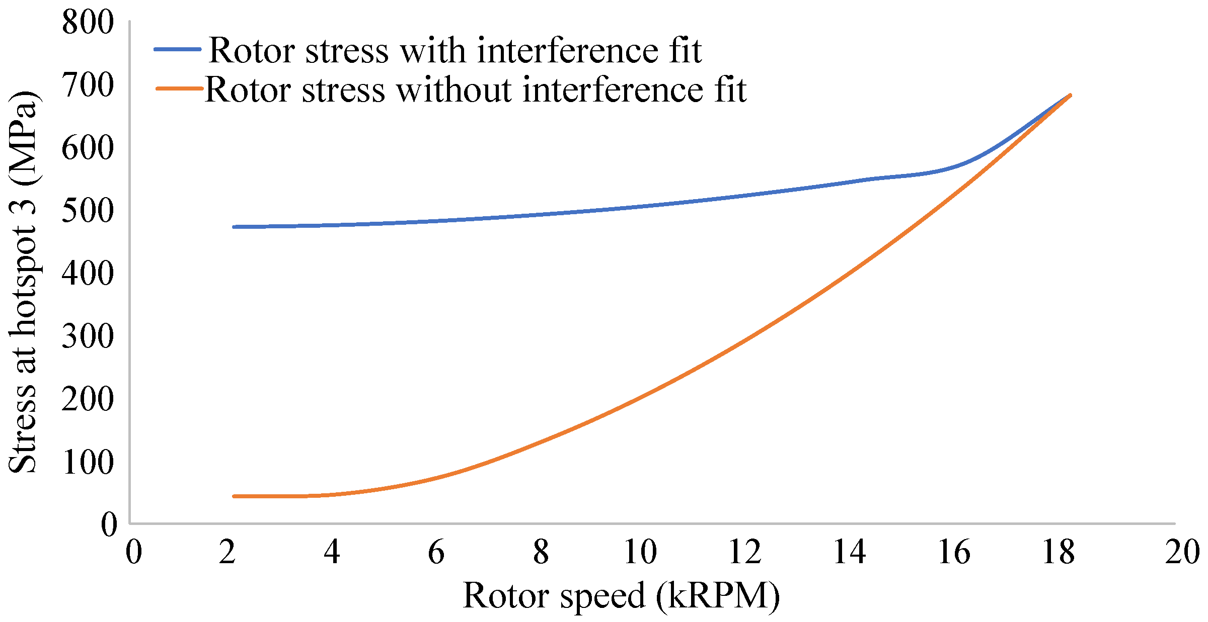
Next, a stress analysis is carried out considering a rotor speed of 18,000 RPM, a 30 micron interference fit between the rotor and shaft, and the rotor, shaft, and magnet temperature at 150 °C.

The von Mises stress levels at Hotspot 3 due to thermal and centrifugal loads, considering scenarios with and without an interference fit, are compared in Figure 2. When the interference fit is taken into account, the stress at Hotspot 3 maintains a relatively constant value for a majority of the speed range. It is only after reaching a speed of 16,000 RPM that the centrifugal load begins to exert greater influence, surpassing the effects of the interference fit. This observation implies that Hotspot 3 has high mean stress during a drive cycle as compared to Hotspots 1, 4, and 5.

In Figure 3, the von Mises and the maximum principal stress normalized to yield strength are compared for all hotspots. The von Mises stress, which is based on the maximum distortion energy theory, is observed for ductile materials such as electrical steels because it ensures no permanent deformation if the induced stress is below the yield strength.

The induced stress on a component can also be classified as tensile or compressive. The tensile stress is due to the pulling nature of the load, whereas the compressive stress is due to the compressive behavior of the load. Experiments suggest that a compressive mean stress is favorable and a tensile mean stress is unfavorable to fatigue life [20]. Therefore, it is a good practice to check the maximum principal stress because there can be hotspots with a high von Mises stress and compressive behavior, which may lead to a superior fatigue life as compared to a high von Mises stress and tensile behavior.

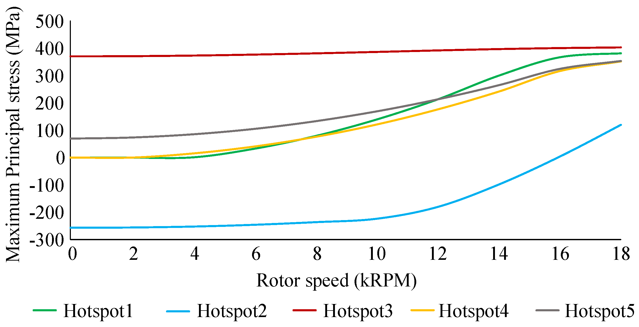
As shown in Figure 3a,b, all hotspots have high von Mises stress, and all of them are under tensile conditions at the maximum speed of the rotor. The maximum principal stress is positive when the stress has a tensile behavior. As shown in Figure 4, the initial temperature and interference fit has negligible impact on Hotspots 1 and 4, a minor tensile effect on Hotspot 5, a significant tensile effect on Hotspot 3, and a significant compressive effect on Hotspot 2. As the centrifugal force increases with speed, the centrifugal load overpowers stress due to interference fit at Hotspot 2, leading to a tensile maximum principal stress at higher speeds, as shown in Figure 4.

3. Drive Cycle Design for Thermomechanical Fatigue Analysis of a Rotor

The drive cycle holds significant importance for the design and development of any motor, as it defines a crucial target for motor operating points. These drive cycles are typically derived from real-world usage patterns. In the context of this paper, a daily transient velocity drive cycle is created using generic drive cycles to replicate the real-world usage pattern and assess the rotor fatigue life [27].

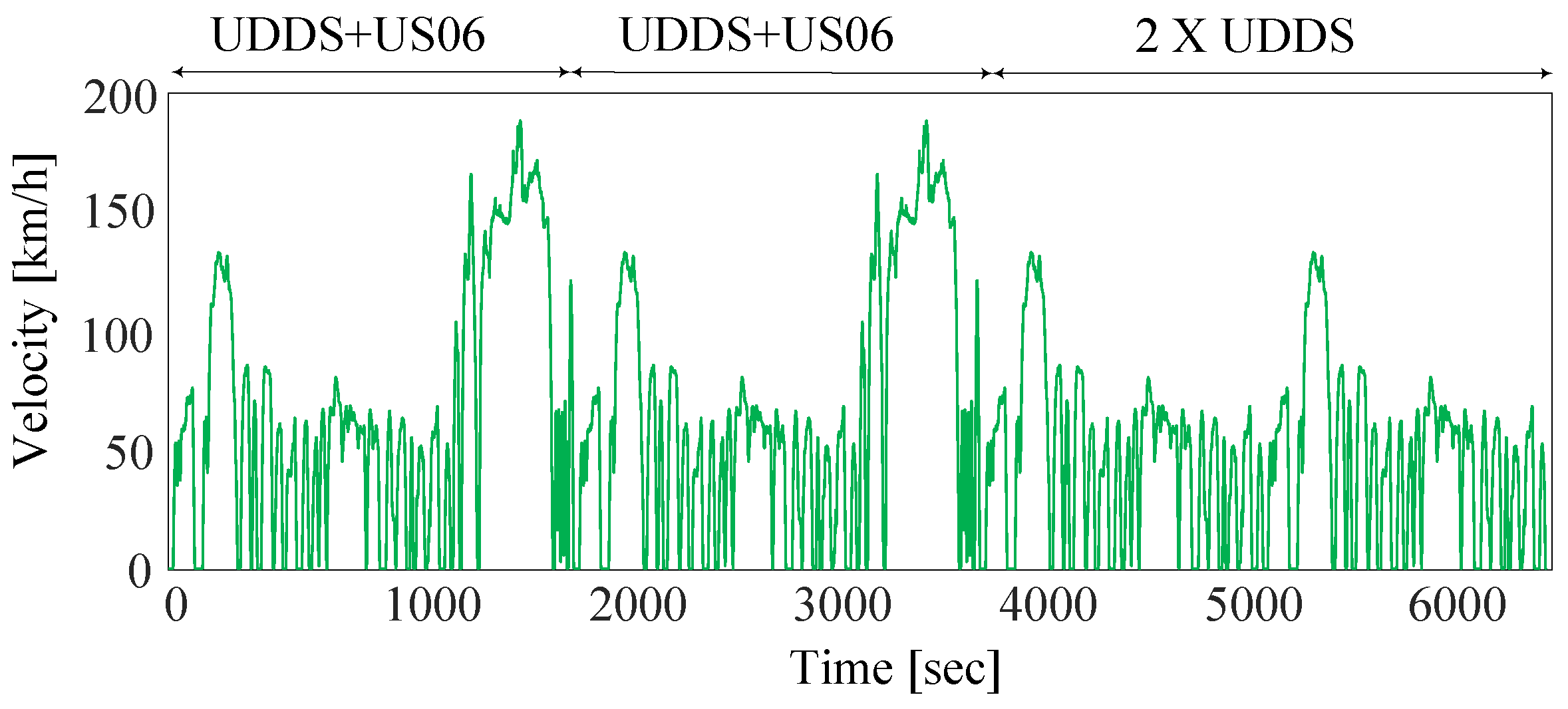
It is assumed that that vehicle is driven for a round-trip commute to the workplace, followed by an evening excursion. The round-trip office commute is represented through a combined sequence of the Urban Dynamometer Driving Schedule (UDDS) and the US06 Emission Test Cycle. Similarly, the evening excursion is represented by the UDDS cycle. The drive cycle is scaled by 50% to make it more demanding for durability requirements. This ensures that the rotor speed reaches the peak rotation speed during the drive [13].

Generic drive cycles are constructed based on vehicle velocity to evaluate overall vehicle performance. So, the daily transient velocity drive cycle shown in Figure 5 is converted to the daily motor speed profile using a vehicle wheel diameter and a gear reduction ratio between the electric motor and the wheels. The daily transient velocity drive cycle is then used to conduct the thermal analysis of the motor, and the daily motor speed profile is used to carry out a thermomechanical fatigue analysis of the rotor.

4. Motor Thermal Management and Temperature Profile Estimation for a Drive Cycle

Maintaining the magnet and coil temperatures below critical thresholds through an effective cooling mechanism holds a pivotal role in optimizing the motor performance. In addition, driving dynamics change continuously and rapidly for a drive cycle, which impacts the thermal performance significantly. In turn, this leads to a fluctuation in rotor assembly temperature throughout the drive cycle. The rotor assembly temperature fluctuation leads to a variations in mechanical and fatigue properties. Therefore, it is critical to evaluate the rotor assembly temperature for the drive cycle. The Ansys Motor-CAD is used at this stage to calculate the rotor temperature profile for a given drive cycle.

First, electromagnetic (EM) analysis is carried out to calculate the motor loss, and a loss model is built for the entire speed range. Then, a hybrid cooling system is modeled for the thermal management of the motor, which consists of a cooling water jacket, oil spray on end windings, and oil flow through the shaft.

An initial motor temperature, an inlet water temperature, and an inlet oil temperature are considered based on normal operating conditions. An average electric motor temperature is expected to be around 100 °C under normal operating conditions. Typically, a vehicle-level cooling system for an electric drive train may consist of an electric motor heat exchanger, which supplies coolant at around 65–67 °C. Therefore, the inlet water temperature is considered to be 70 °C, assuming a 3–5 °C rise until the coolant reaches the inlet of the motor water jacket. For a hybrid cooling system, the coolant passes through the water jacket to an oil cooler, leading to an oil cooler temperature around 75–77 °C. Assuming an increase of 3–5 °C in the oil until it reaches the oil spray and shaft inlet, 80 °C is considered to be the oil inlet temperature.

Simulations are conducted for the entire speed range for 30 s of peak power operations to ensure that the heat capacity of the motor is sufficient, and for steady-state conditions to ensure that the heat dissipation capacity is sufficient for continuous operations. 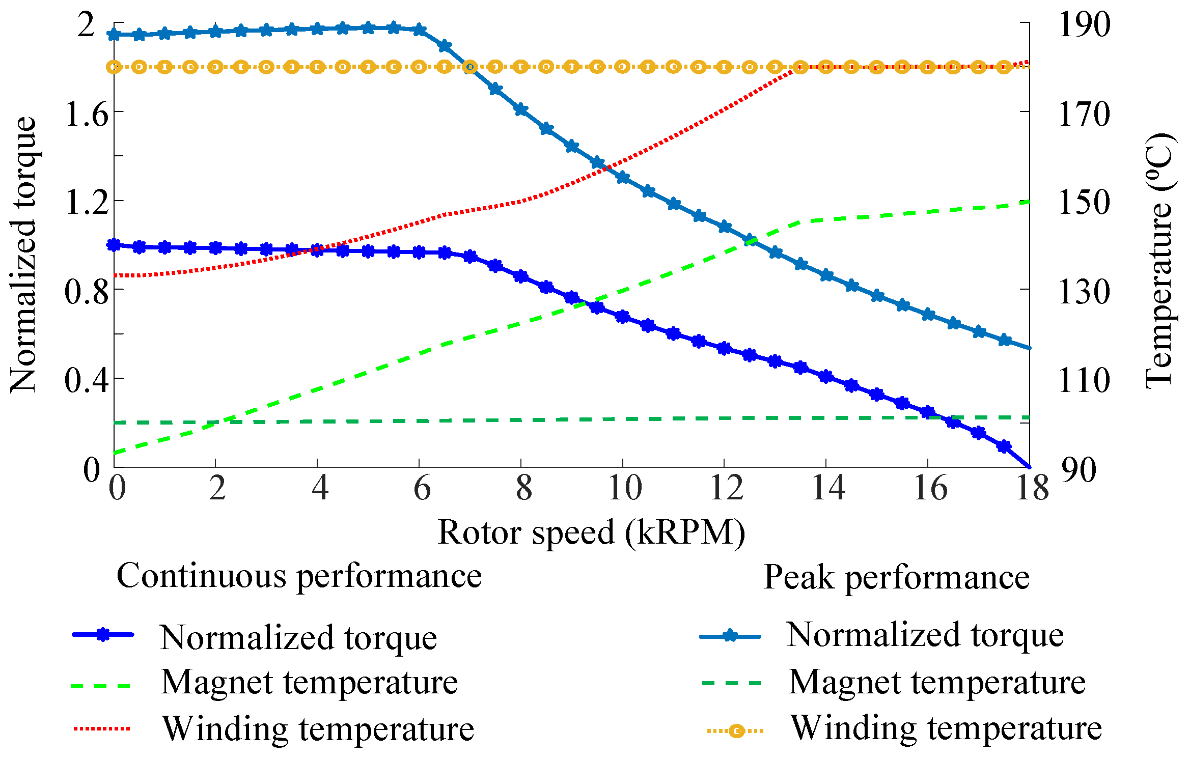The volume flow rate of the coolant is 12 LPM for the water jacket, 3 LPM for the oil spray, and 3 LPM for the oil flow through the shaft to maintain the magnet and coil temperature below 150 °C and 180 °C [28], respectively. The per-unit torque, magnet, and coil temperature for the continuous and the peak performance as well as the entire speed range after the tuning of the cooling model are shown in Figure 6.

The magnet and the winding temperature during operation depend on their losses, heat flux from adjacent components, and initial temperature conditions. During a 30 s peak power operation, there is insufficient time for heat to transfer between components. As a result, the magnet temperature remains closer to its initial condition, mainly because magnet losses are negligible. In contrast, during steady-state continuous operation, the magnet temperature tends to be higher due to heat accumulation. The winding and core losses increase with speed, so the magnet temperature increases with an increase in speed.

The winding temperature during the 30 s peak power operation across various speeds is consistently at 180 °C, primarily due to the high current applied to the conductors. This temperature serves as a limiting factor for peak power operation, and the current is optimized to keep the winding temperature within limits while delivering maximum power. In steady-state continuous operation, the lower current at lower speeds keeps the winding temperature lower. However, as speed increases, copper losses rise, causing the winding temperature to gradually approach the maximum allowable limit.

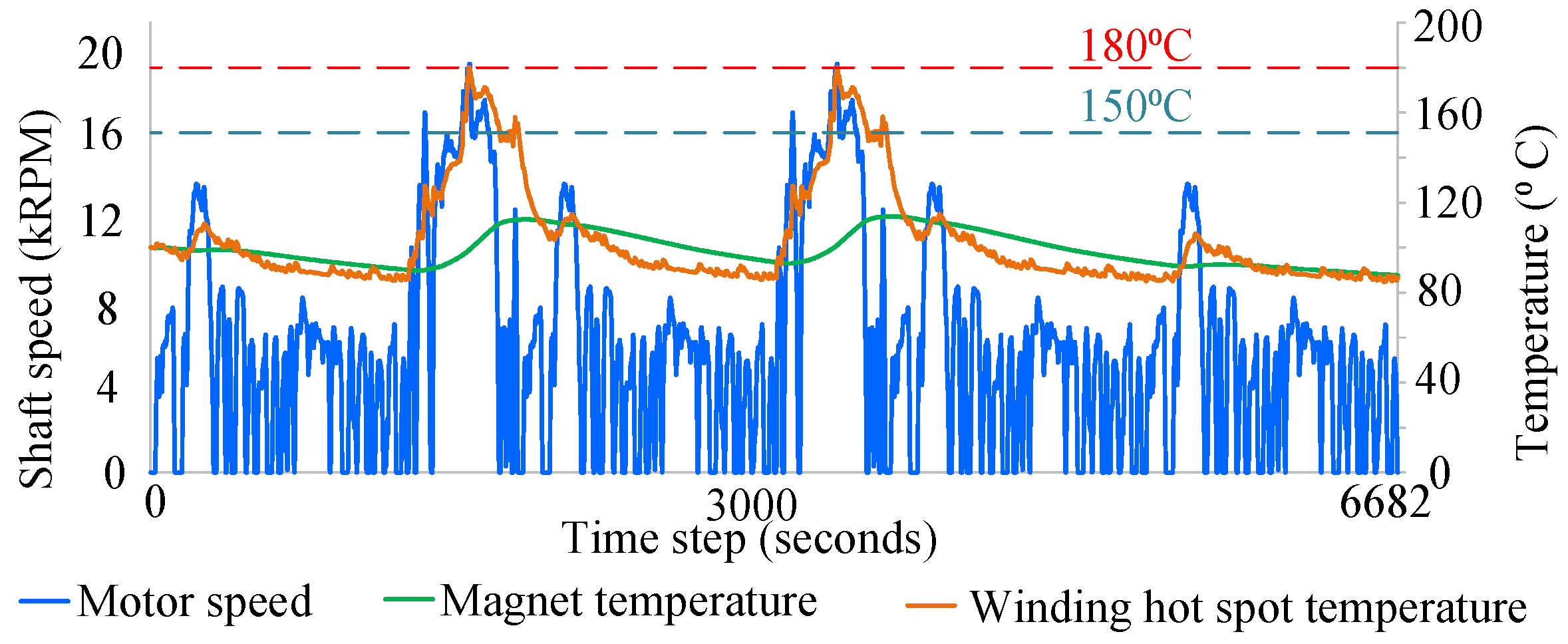
Figure 7 shows the rotor temperature profile for the daily drive cycle. The temperatures are calculated from the thermal model of the motor by applying the electromagnetic motor losses. In order to capture the worst-case scenario, the rotor temperature is calculated without any vehicle stops.

5. Accelerated Fatigue Life Approach

Estimating stress and fatigue for a drive cycle can be computationally expensive, as it requires a stress- and fatigue-life estimation at each time step. Deterministic events like drive cycles have defined loads for each time step. Accelerated fatigue-life approaches such as load amplification, peak valley extraction, and block cycles can be used to accelerate fatigue-life estimation for deterministic events [16]. In this paper, the peak–valley extraction method is applied to remove the non-damaging time steps from the drive cycle, which is then used to carry out the rotor stress and fatigue analysis.

The stress values only at troughs and crests of the drive cycle are critical for fatigue life estimation [29,30]. Therefore, the intermediate rotor speed values can be removed, and consequently, a compressed drive cycle can be used for the rotor fatigue to reduce the simulation time. The peak–valley approach conserves the load amplitude and sequence information but does not conserve the frequency information [29]. Frequency information is critical if dynamic inertial loads induce stress. Dynamic inertial loads are caused by self-weight under resonance, and their intensity depends on the frequency. In the case of rotor assembly, the natural frequency is much higher than the frequency of centrifugal force fluctuation acting on the rotor. The dynamic effects can be neglected if the excitation frequency is twice the system’s natural frequency [31].

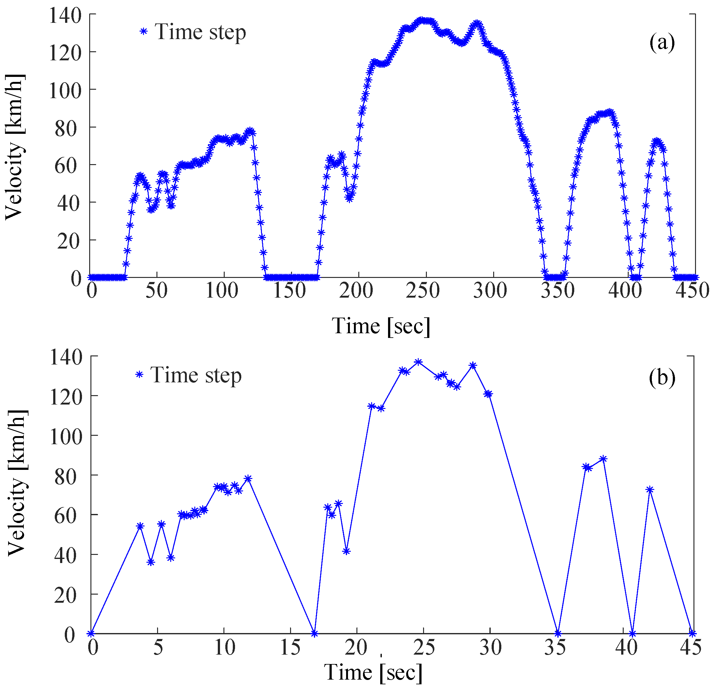
The software nCode GlyphWorks is used to remove the non-damaging time steps from the daily rotor speed profile. Three consecutive data points are checked to see if the middle data point is greater than the adjacent data point, and then the non-peak or non-valley point is discarded. The first 450 time steps from the original daily rotor speed profile are compressed to 45 time steps in the compressed drive cycle, as shown in Figure 8a,b. The full drive cycle data are compressed from 6682 time steps to 792 steps. The rotor temperature calculated earlier for the original drive cycles is also updated based on the compressed drive cycle.

6. Rotor Stress Analysis for a Drive Cycle

So far, we have explored the effect of different loads on rotor laminations, developed the rotor temperature profile for the drive cycle, and compressed the drive cycle to reduce the simulation time. This section presents the calculations for the prediction of the stress the rotor experiences throughout the drive cycle. This is important for determining how long the rotor can last before developing a crack. In an electric motor, the rotor stress can be induced due to the combined thermal load, interference fit, and centrifugal load, which are all considered in this paper. The stress induced by the electromagnetic load is much smaller than the other loads, so it is not considered for rotor stress analysis.

For the stress analysis, boundary conditions presented in Figure 1 are applied. The centrifugal load used in the stress analysis is based on the daily motor speed profile, and rotor, magnet, and shaft temperature profiles are based on the daily velocity drive cycle shown in Figure 9.

Material nonlinearity should account for plastic deformations when the stress induced during a drive cycle is higher than the yield strength. Additionally, finite element analysis with nonlinear material characteristics is preferred for structures with complicated boundary conditions, materials, and loading conditions [32].

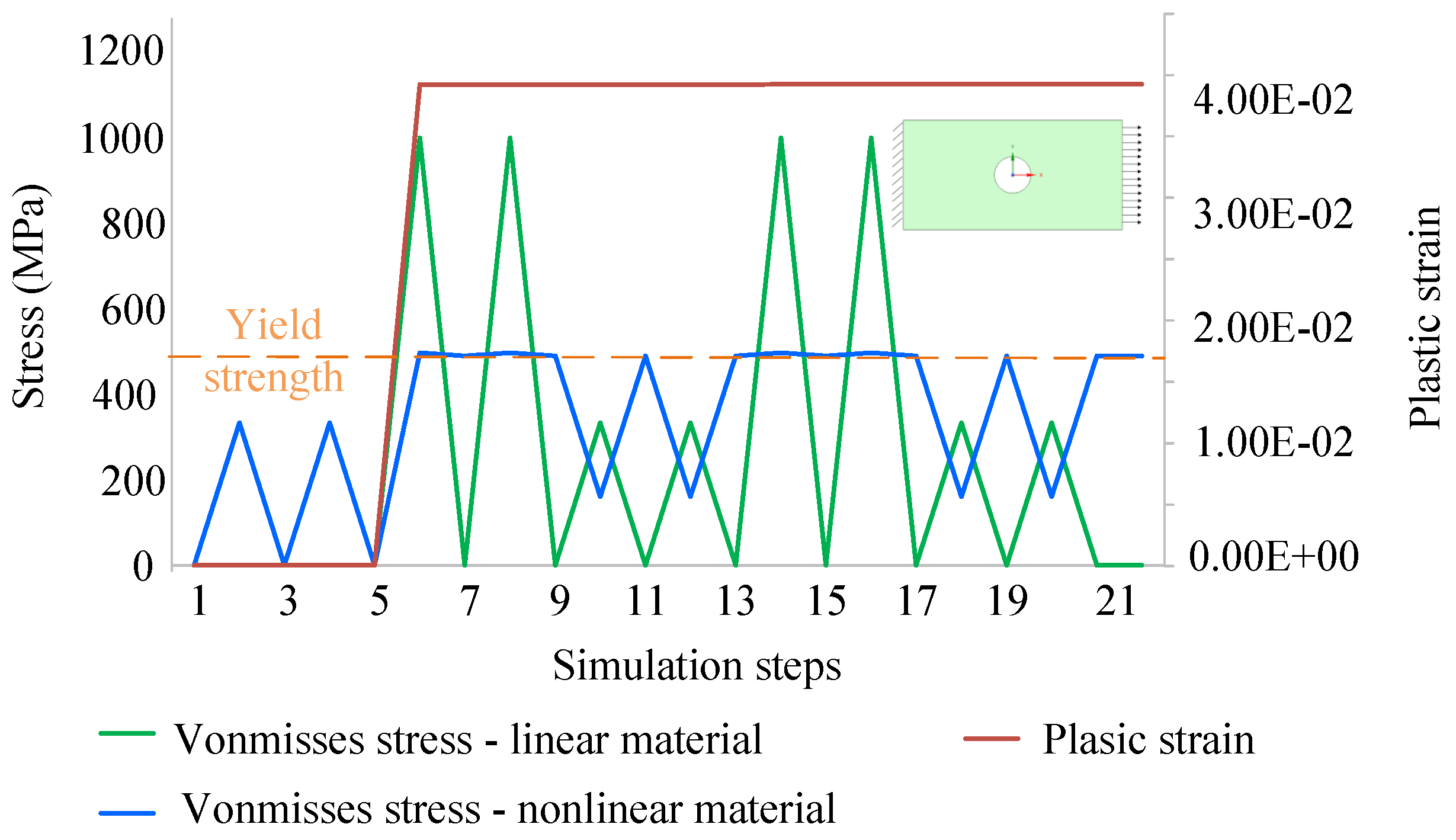
In order to comprehend the stress difference between a linear and a nonlinear material, a simple geometry of a plate with a hole is investigated. The inset in Figure 10 shows the geometry considered. This geometry is chosen for this investigation because it resembles the stress hotspots of a rotor air flux barrier with notches. A variable pulsating load is applied at one end, and the other end is fixed. Linear material properties are modeled using the modulus of elasticity, which calculates stress accurately if the stress is below the yield strength. Above yield strength, it over-predicts the stress, which is why it is also called pseudo-stress. Nonlinear material properties are modeled using a true stress–true strain curve in addition to the modulus of elasticity. The true stress–true strain curve captures the elastoplastic behavior of the material beyond the yield strength. So, the stress above yield strength is predicted accurately with nonlinear material properties. As shown in Figure 10, the stress induced with linear and nonlinear material properties matches between simulation steps 1–5, when the stress is below the yield strength.

Plastic strain induced when the stress is higher than the yield strength is called a permanent set, and it remains permanent even when the stress after that reduces below the yield strength. Once the stress is beyond the yield strength of the material, the permanent set causes deviation in stress prediction even for the instances where the stress is below the yield strength. As shown in Figure 10, the stress induced is above yield strength at simulation step 6. The difference in the linear and nonlinear stress is due to the difference in the characteristics of the linear and nonlinear material modeling. A permanent set of 0.04 is also induced at simulation step 6 for nonlinear simulation. The nonlinear stress between simulation steps 9–10 varies from the linear stress because of the permanent set, even though it is below yield strength.

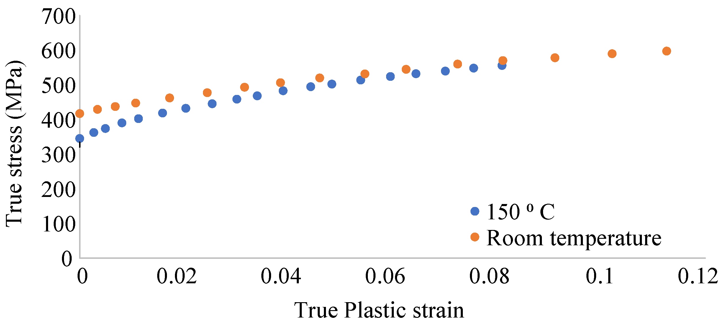
The Ansys Mechanical software is used for the stress analysis for the daily rotor speed profile. Mechanical properties are required for at least two temperatures to carry out the thermomechanical simulation. The 27PNX1350 electrical steel is selected for the analysis, whose mechanical properties, along with the nonlinear stress–strain curve, are available at room temperature and at 150 °C [14]. Since the object of investigation is rotor lamination failure, nonlinear material is used only for the electrical steel. The true stress–true plastic strain curve in Figure 11 is used to model the material nonlinearity as per the requirement of the finite element software. 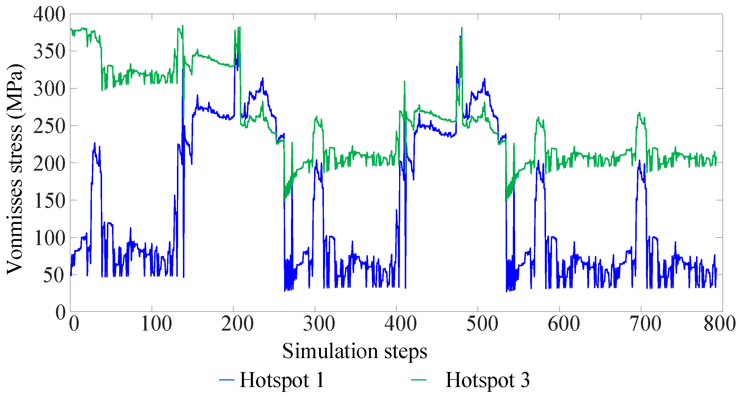The adhesive modulus of elasticity is used from [26]. The von Mises rotor stress for Hotspots 1 and 3 in Figure 1 is shown in Figure 12. It is evident that the interference fit significantly impacts regions near the interface between the rotor and shaft. Consequently, the mean stress levels are considerably higher at Hotspot 3 compared to Hotspot 1 over the entire duration of the daily rotor speed profile. In contrast, the amplitude stress experienced at Hotspot 1 is notably higher compared to Hotspot 3.

7. Thermomechanical Fatigue Analysis

Once the rotor stress results are available for the daily rotor speed profile, fatigue analysis is carried out in nCode DesignLife. A temperature-dependent S-N curve for 27PNX1350 electrical steel is generated in the nCode MaterialsManager. The stress amplitude intercept and a slope of 1 are used from the experimental data available in [14], and the endurance strength, the stress at fatigue cut-off limit, and a slope of 2 are derived with empirical calculations [32]. Temperature-dependent fatigue properties are used based on the rotor temperature profile to carry out the fatigue analysis at each time step. This analysis shows how well the rotor holds up under real-world driving conditions.

7.1. Stress-Life Curve Generation

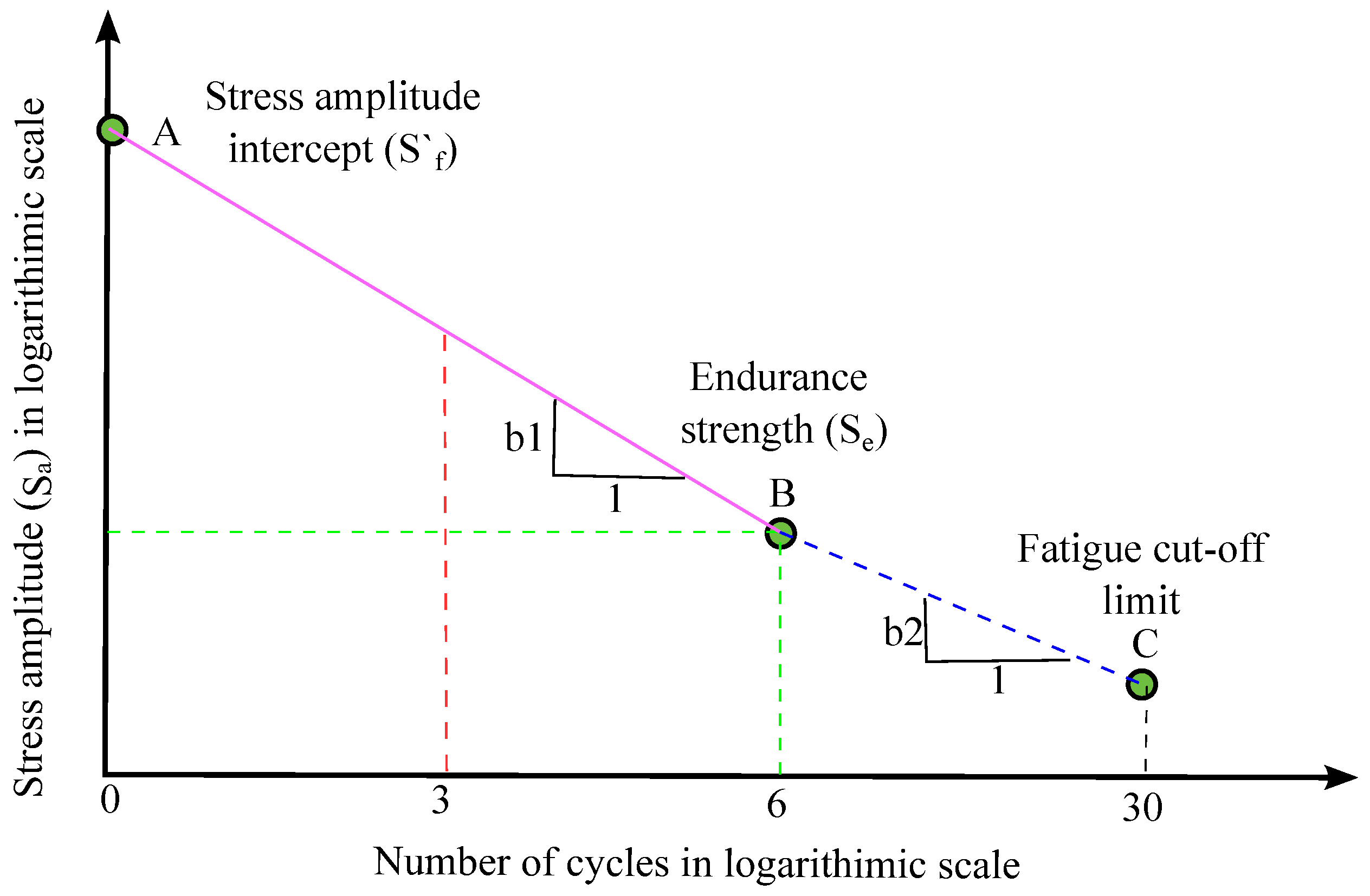
In a high-cycle fatigue regime, the S-N (stress-life) curve for steel material is typically represented on a logarithmic scale, as illustrated in Figure 13, where the y-axis displays the stress amplitude, and the x-axis shows the number of cycles until failure. High-cycle fatigue regimes are usually considered when the number of cycles exceeds ${10}^3$ or when fatigue damage is due to little or no plastic deformation [32]. For a constant amplitude loading, typically line AB in Figure 13 is considered, where point A is the stress amplitude intercept, and point B is called the endurance strength. The line is considered horizontal after the endurance strength, which means infinite life if the induced amplitude stress is below endurance strength. The stress amplitude intercept is the stress that would lead to failure at 1 cycle, and $b1$ is the slope of the line AB.

In cases of variable amplitude loading, it is crucial to note that stress cycles below the endurance limit can still cause damage if some of the cycles under variable loading have stress levels above endurance strength. To address this, the S-N curve is extended to point C, known as the cut-off point [32]. The slope $b2$ is computed from the slope $b1$, as outlined in Equation (1):

$$b2=b1/(2+b1).$$

(1)

The S-N curve can be expressed in equation form, as outlined in Equation (2):

$$Lo{g}_{10}\left(S_a\right)=Lo{g}_{10}\left({S^{\prime }}_f\right)+b Lo{g}_{10}\left(N\right).$$

(2)

Here, $S_a$ is the induced stress amplitude, ${S^{\prime }}_f$ is the stress amplitude intercept, b is the slope of the line, and N is the number of cycles until failure for the induced stress amplitude.

We obtain slope $b1$ and the stress amplitude intercept from [33], which were experimentally derived using dumbbell-shaped specimens of thin electrical steel sheets. Subsequently, we calculate the endurance strength, the stress at the cutoff point, and the slope $b2$ using Equations (1) and (2).

Table 3. Median stress-life parameters of 27PNX1350 at room temperature and 150 °C.

Parameter	Value	Temperature
Stress amplitude intercept (${S^{\prime }}_f$)	1502.3 (MPa)	RT
Slope 1 ($b1$)	−0.12	RT
Slope 2 ($b2$)	−0.06383	RT
Endurance strength ($S_e$)	286.2 (MPa)	RT
Stress at fatigue cut-off limit	8.4 (MPa)	RT
Stress amplitude intercept (${S^{\prime }}_f$)	1236.7 (MPa)	150 °C
Slope 1 ($b1$)	−0.112	150 °C
Slope 2 ($b2$)	−0.05932	150 °C
Endurance strength ($S_e$)	263.2 (MPa)	150 °C
Stress at fatigue cut-off limit	9.9 (MPa)	150 °C

consolidates the parameters used for generating the median S-N curve at both room temperature and 150 °C. The parameters applied in this analysis are based on median values derived from multiple samples of experimental data. It signifies that only 50% of the samples would meet the expected fatigue life under the drive cycle operation. These data form the basis for our fatigue analysis, allowing us to assess material performance under varying load conditions of a drive cycle.

7.2. Fatigue Analysis Results

In the context of fatigue analysis, several crucial considerations extend beyond the assessment of drive cycle stress and material fatigue properties. In the high-cycles fatigue regime, a mean stress has a significant effect on the fatigue behavior [32]. The S-N curve generated for a stress ratio −1 takes into consideration the impact of stress amplitude fluctuations. To account for the influence of mean stress, the Goodman mean stress correction criterion is applied because it is considered to be the most conservative approach [18]. Stress ratio is the ratio of maximum to minimum stress for a stress cycle. The surface roughness is another key factor that affects fatigue life. Rotor lamination can be manufactured by various manufacturing processes, such as laser cut or shear cut, which significantly influence the surface roughness of rotor lamination edges [33,34,35]. The S-N curve employed in our analysis is derived from samples prepared using the computer numerical control (CNC) technique [14], and it inherently incorporates the effects of surface roughness.

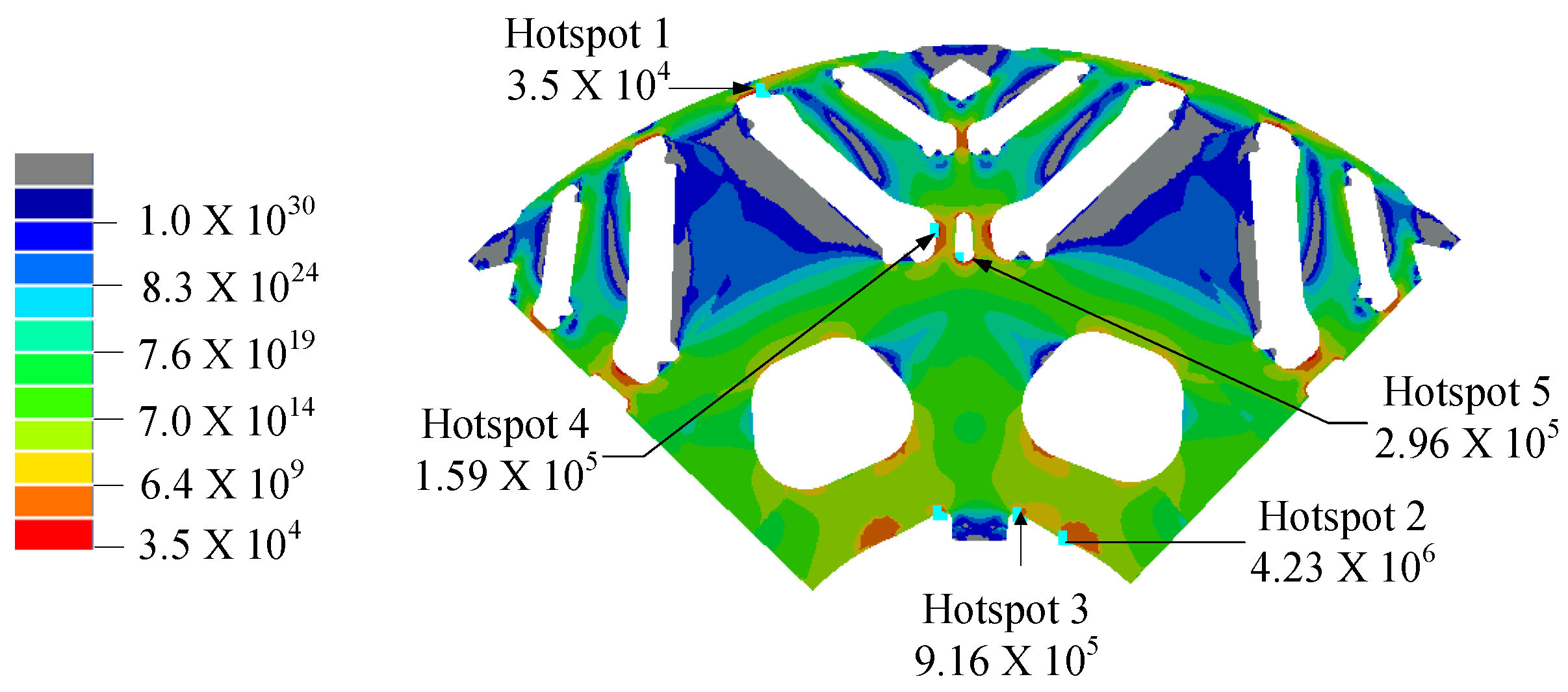
The fatigue life analysis for the rotor lamination, accounting for varying loads, a temperature-dependent S-N curve, and the Goodman mean stress correction factor, is shown in Figure 14. The contour plot depicting fatigue life ranges from the minimum observed value up to the cutoff limit and beyond. Notably, the minimum fatigue life is observed at Hotspot 1, amounting to $3.5\times {10}^4$ daily drive cycles, equivalent to approximately 95 years of operation. It is also observed that the fatigue life at Hotspot 3 is higher than that at Hotspots 1, 4, and 5. This implies that the combined effect of higher mean stress and lower amplitude stress may be less detrimental than the scenario with higher amplitude stress and lower mean stress concerning rotor fatigue under the defined drive cycle. Interestingly, Hotspot 2 exhibits the highest fatigue life among all the hotspots, possibly attributed to the compressive nature of stress experienced in this region.

As previously discussed, the fatigue results presented in Figure 14 are derived from fatigue properties based on the median value of experimental data. Estimating fatigue with it may lead to 50% of the samples failing under drive cycle operation. Moreover, the data are based on a limited number of samples, so confidence in the data is also low. For the design of critical components, the S-N curve should lie on the lower or safer side of the data. The curve is often modified based on the standard deviation to meet the 90% confidence and 95% reliability criteria, referred to as the R90C95 S-N curve [36,37]. In practical terms, this means that rotor designs based on the R90C95 S-N curve have a 90% probability that 95% of the samples will successfully complete the drive cycle operation without encountering fatigue failure.

Table 4. R90C95 stress-life parameters of 27PNX1350 at room temperature and 150 °C.

Parameter	Value	Temperature
Stress amplitude intercept (${S^{\prime }}_f$)	1224 (MPa)	RT
Endurance strength ($S_e$)	192.5 (MPa)	RT
Stress at fatigue cutoff limit	3.7 (MPa)	RT
Stress amplitude intercept (${S^{\prime }}_f$)	1195.7 (MPa)	150 °C
Endurance strength ($S_e$)	188.2 (MPa)	150 °C
Stress at fatigue cutoff limit	3.6 (MPa)	150 °C

shows the fatigue parameters for the R90C95 S-N curve for 27PNX1350 electrical steel [14], where the slope remains the same as the median S-N curve. The minimum fatigue life observed for rotor lamination at Hotspot 1 is $1.93\times {10}^4$ daily drive cycles, which is approximately 44% lower than the fatigue life calculated using the median S-N curve.

8. Conclusions

This paper proposes a thermomechanical accelerated fatigue analysis approach for an IPMSM rotor. The rotor stress analysis modeling is discussed, along with loads and boundary conditions. Then, various loads acting on the rotor are investigated. It is found that the stress induced due to a thermal load, a centrifugal load, and an interference fit may be significantly higher than the electromagnetic stress. Then, a vehicle velocity drive cycle is created, and the thermal management of the motor is defined through simulations. It is ensured that the magnet and coil temperatures are maintained below the critical temperature during continuous and peak operating conditions. Then, the peak–valley extraction method is applied to remove the non-damaging cycle, which helps to reduce simulation time by approximately 90%. Then, the rotor stress analysis is carried out for the drive cycle, using a nonlinear simulation approach based on the true stress–true plastic strain curve drive from a strength test of thin electrical steel. The rotor thermomechanical fatigue analysis is then carried out for the drive cycle using a median S-N curve and considering the mean stress effect. The minimum fatigue life observed on the rotor lamination is approximately 95 years of drive cycle operation. The rotor lamination fatigue life is also calculated for the R90C95 S-N curve, which shows a 44% reduction in fatigue life as compared to the median S-N curve.