Abstract
Mobile robots can replace humans to fulfill tasks in dangerous environments, which has been a research focus in recent years. This paper proposes a wheel-legged mobile robot with multi-locomotion and a low-energy consumption planning method. Different from the existing wheel-legged mobile robots, it can realize low-energy movement in different terrains with simple structures, and it can realize three modes: synchronous, tumbling, and curl–stretch. Then, based on the kinematics and dynamics model, a low-energy planning method is proposed, and low-energy motion planning is carried out for the three modes to obtain the low-energy driving law in each mode. A robot prototype is developed, and the experimental results show that the robot can move through the three modes with lower energy consumption in all three terrains. The planning method provides an effective reference for applying wheel-legged mobile robots.
1. Introduction
Mobile robots are widely used in military reconnaissance and energy exploration [1,2,3]. Traditional mobile robots use wheeled [4,5], legged [6,7,8], or tracked [9,10] traveling mechanisms, which only have an advantage in maneuverability or obstacle-crossing performance, making it challenging to consider both characteristics. They cannot adapt to complex environments and feature high energy consumption when facing specific environments. To address the problem of poor terrain adaptability, some scholars proposed the concept of combining wheels and legs in the same traveling mechanism and designed the wheel-legged mobile robot [11,12,13,14,15,16,17]. Typical examples of wheel-legged mobile robots are RHex series robots [18,19,20,21,22,23,24,25], Whegs series robots [26,27,28,29,30,31], and Asgard series robots [32], in which circular wheels are transformed into discrete fork forms. These wheel-legged mobile robots greatly simplify the overall structure, lower the control difficulty, and increase terrain adaptability. However, wheel-leg robots often cannot play their role when facing some types of terrain. Also, the robots consume a lot of energy due to the control method. Given the above problems, some scholars have proposed adding motors or unique mechanisms to make a robot switch between the two states of wheeled and legged forms, realizing a variety of modes to improve robot performance. The ATHLETE robot [33], PAW robot [34], and Rolling-Wolf robot [35] are typical representatives. The wheel–leg-integrated mobile robot solves the maneuverability and obstacle-crossing problems of the legged structure, expands terrain adaptability, and reduces energy consumption by adding a switching device between the wheels and legs. However, it increases the difficulty of structural design and does not propose a low-energy control method for legged movement, so the energy consumption of the robot is still high when it moves in the legged mode.
Aiming at the shortcomings in the current research, this paper proposes a low-energy wheel-legged mobile robot with a variable body. The kinematics and dynamics model of the robot are established, and a low-energy planning method is proposed for low-energy multi-locomotion planning. On this basis, the energy consumption of the robot on flat ground, soft ground, and downhill is analyzed. The influence of the motion mode and driving law on the mechanical energy consumption of the robot when it moves in different terrains is also studied. Finally, the effectiveness of the planning method and low-energy motion planning is verified by experiments.
2. Structure Design
The wheel–leg structure designed in this paper is shown in Figure 1. The shape parameters include the spoke chord length the spoke radius of curvature , and the number of spokes, which is three. The angle between the spokes is the same. The spoke shapes of the wheel-legs investigated in this paper are all inferior arcs. The chord length is taken as the primary dimension. The parameters are shown in Table 1.
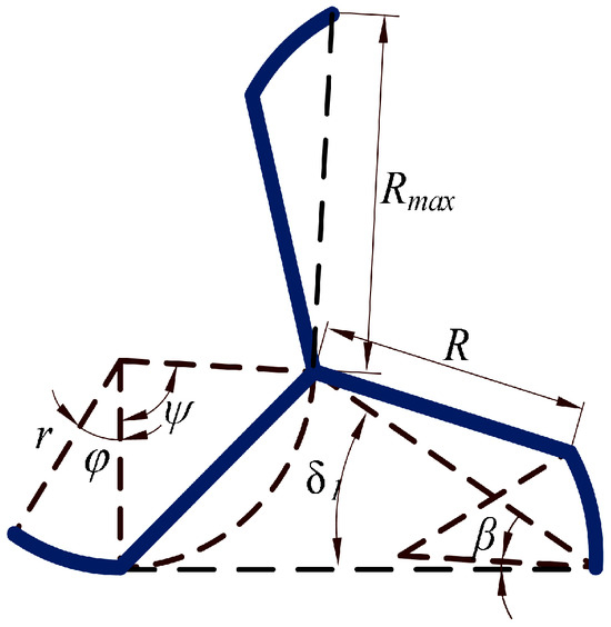
Figure 1.
Sketch of the wheel-leg structure.

Table 1.
Parameters of the wheel-leg.
The robot’s structure is shown in Figure 2. The body is made of five connecting rods with a length of 25 mm, and the drive and electronic components, etc., are arranged inside the body.
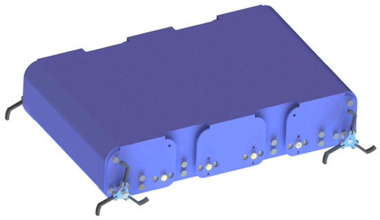
Figure 2.
Robot’s structure.
3. Modeling
In contrast to general wheel-legged mobile robots, the wheel-legged robot proposed in this paper can realize multiple modes through body deformation and wheel-leg rotation to adapt to different terrains. In particular, the robot’s body deformation and the wheel-leg’s rotation are controlled by the angle of the drive [36,37]. The kinematic and dynamic models of the robot are derived in this section [38].
3.1. Kinematics Model
The following assumptions are made: the center of gravity of the wheel-legged mobile robot parts is located at the geometric center of the parts; the body is symmetrically distributed to the geometric center; and it is assumed that there is no longitudinal slip and transverse slip during the robot’s motion.
From Figure 3, it can be seen that each joint angle of the robot body satisfies:
where represents the angle between rod Ai−1Ai and AiAi+1 (i = 2~5); (i = i~2) represents the angle between rod AiAi+1 and A2A4; and (i = i~3) represents the angle between rod A3A4 and A2A4, rod A2A4 and A4A6, and rod A4A5 and A4A6.
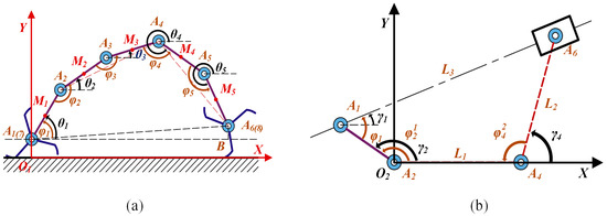
Figure 3.
Mechanism sketches. (a) Mechanism sketch of the robot. (b) Mechanical sketch of a part of the robot body.
Equation (2) can be obtained by projecting onto the X- and Y-axes:
where γi (i = 1, 2, 4) represents the angle between A1A2, A1A6, and A4A6 and the positive direction of the X-axis; L1, L2, and L3 represent the length of L1, L2, and L3, respectively; and L represents the length of rod AiAi+1 (i = 1~5).
Solving (3) gives:
Equations (6) and (7) can be obtained by bringing the geometrical relations in Figure 3 into Equations (4) and (5):
The displacement of point A6 in the plane can be expressed as
The projection of Equation (8) onto the coordinate axes can be expressed as
where θi represents the angle between the rod AiAi+1 (i = 1~5) and the X-axis; A1 and A6 are points on the body; xA1(yA1) represents the displacement of point A1 on the X(Y)-axis; and xA6(yA6) is the displacement of point A6 on the X(Y)-axis. Based on Figure 3a, we have:
where represents the angle between A1A6 and A1B; yA8 represents the displacement in the Y-axis direction of the front wheel-leg, and yA7 represents the displacement produced by the rear wheel-leg in the Y-axis direction.
The wheel-leg structure is shown in Figure 1; the four wheel-legs of the robot are the same size. When the wheel-legs rotate clockwise, the center point of the wheel-legs A7(A8) in the X-axis and Y-axis displacements of a cycle of displacement can be expressed as Equations (12) and (13):
where
where s1 is the distance traveled in the first stage when the wheel-leg is turned clockwise.
The velocity equation can be obtained for the center point of the wheel-leg A7(A8) displaced by one cycle in the X-axis and Y-axis:
where and are the robot’s velocities in the X-axis and Y-axis directions.
For there to be no relative sliding between the wheel-legs and the ground during the movement of the robot, the point A1(A6) point on the body should be displaced in the same way as the point A7(A8) point on the wheel-leg:
By bringing Equation (17) into Equation (9), we have:
where θi (i = 7~8) is the turning angle of the wheel-leg.
Combining Equations (9)–(13) yields a parametric expression for the displacement of point Mi on the robot as
where xi, yi is the displacement of point Mi(i = 1~5) in the direction of the X-axis and Y-axis. and are 0 when j > i − 1.
From Equation (19), the velocity equations of Mi(i = 1~5) in the direction of the X-axis and Y-axis can be obtained as
where , is the displacement of point Mi(i = 1~5) in the direction of the X-axis and Y-axis. and are 0 when j > i − 1.
3.2. Dynamics Model
The dynamics of the robot is modeled by Lagrange’s dynamical equations:
where L equals the kinetic energy minus the potential energy of the robot. The displacements and velocities of the joints and parts of the robot were solved in the previous section, so the total kinetic energy of the robot can be expressed as:
where mi represents the mass of the ith linkage of the robot, Ji represents the rotational inertia of the ith linkage of the robot, mA7 represents the mass of the wheel-leg, and JA7 represents the rotational inertia of the wheel-leg.
The gravitational potential energy of the robot can be expressed as
Based on Equations (21)–(23), the drive joint torque τi can be solved.
The mechanical power during robot motion is:
Based on the DC motor characteristic curve, it is known that the torque of the DC motor is proportional to the current. Therefore, the actual mechanical energy consumption of the robot in one cycle of motion is:
where ET represents the energy consumed by the robot per unit distance, S represents the distance the robot moves in one mode, and α represents the coefficient of proportionality between current and torque.
4. Low-Energy Motion Planning
According to the body structure and the kinematic model, the robot can realize three modes: the synchronized mode, the tumbling mode, and the curl–stretch mode. In this section, low-energy motion planning is carried out for the three modes of the robot, and a low-energy motion method is proposed to obtain the driving law of the robot’s driving angle under each mode to provide a theoretical basis for the subsequent motion control of each mode.
4.1. Synchronized Mode
The angle of the body does not change when the robot is in the synchronized mode. All the wheel-legs have the same initial angle and move periodically with the same angular velocity. The sequence of the robot’s motion on the flat ground is shown in Figure 4. State 2 is the posture of maximum gravitational potential energy of the robot in synchronized mode, and states 1 and 3 are the postures of the minimum gravitational potential energy of the robot.
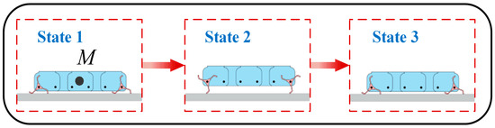
Figure 4.
Locomotion sequence of the synchronized mode.
Therefore, the driving law of the robot in synchronized mode can be obtained as follows:
From Equation (26), it is obtained that a general wheel-legged mobile robot tends to adopt the uniform rotation form of the wheel-legs. The driving law for a single cycle is:
When the robot moves with Equation (27) as the driving law, the robot has the same gravitational potential energy in state 1 and state 3 in one cycle. The wheel-legs collide with the ground at the end of state 3, and the kinetic energy of the robot is almost completely converted into elastic potential energy. Therefore, when the kinetic energy of the robot is 0 in state 2, the mechanical energy consumption of the robot can be reduced. In states 2–3, the drive performs negative work and does not utilize the gravitational potential energy, increasing the energy consumption of the robot. Therefore, relying on gravity to drive the robot at this stage reduces the mechanical energy consumption of the robot.
Based on the above analysis, a driving law is planned in which the work performed by the drive in states 1 and 2 is completely transformed into the gravitational potential energy of the robot, and the robot relies on the work performed by gravity to realize the motion in states 2 and 3. The constraints for the drive turn angle can be obtained as
where t1 is the moment when the wheel-leg rotates to π/2-β.
When t1 = 1, the driving law is fitted with a polynomial. Since there are four known quantities in Equation (28), a cubic polynomial is used to reduce the difficulty of subsequent control. We have:
when t > 1, the robot falls freely, relying on gravity.
Based on Equations (21), (24), (27) and (29), the mechanical power curves of the robot under two synchronized mode drive laws can be obtained, as shown in Figure 5.
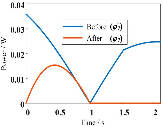
Figure 5.
The mechanical power curve of the synchronized mode.
It can be observed that the overall mechanical power of the robot is reduced. The distance of one cycle of the robot moving in synchronized mode is 2.18 cm. By bringing Equations (27) and (29) into Equation (25) to calculate the mechanical energy consumption of the robot under the two synchronized mode driving laws, respectively, we can obtain the energy consumption of the robot, as shown in Figure 6. The energy consumption before planning is 1.794 J/m and that after planning is 0.461 J/m. The energy consumption ratio of the robot after planning becomes 25.69% of that before planning, and the planning is considered effective.
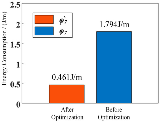
Figure 6.
Mechanical energy consumption of the synchronized mode.
4.2. Tumbling Mode
All wheel-legs are stationary when the robot is in a tumbling mode. The change in the position of the center of gravity after the deformation of the robot’s body moves the robot forward under the effect of gravity. To minimize the impact of inertial forces on the tumbling mode, the robot miniature changes slowly and can be considered to be at rest during tumbling. The locomotion sequence on flat ground is shown in Figure 7.
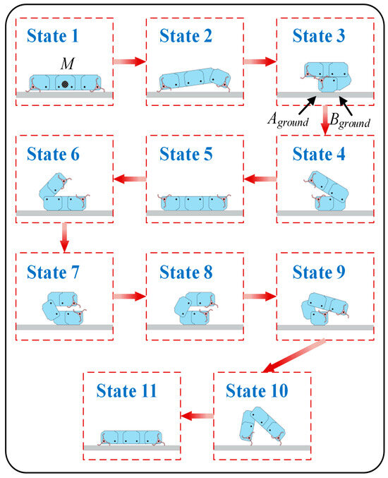
Figure 7.
Locomotion sequence of tumbling mode.
The constraints for realizing the tumbling mode are as follows:
In states 1~3, the robot is lifted by the rotation of the body with the following law:
In states 3~10, to ensure the clockwise rotation of the robot, the direction of the robot’s gravitational moment about Aground must be clockwise; otherwise, the robot will rotate around Aground, causing the motion in states 3~10 to fail. In addition, the direction of the robot’s gravitational moment about Bground must be counterclockwise. Therefore, the constraints for φi (i = 2~5) in states 3~10 are obtained:
In Equation (31), and are the gravitational moments of the robot at Aground and Bground, where Aground and Bground are the robot’s left and right contact points in contact with the ground. In this paper, the gravity moments are negative clockwise and positive counterclockwise. mi is the mass of each part of the robot, and and are the distances of the parts to Aground and Bground.
The driving law for each state can be obtained from Equation (31):
where represents the turning angle of each drive in the previous state, and represents the turning angle that satisfies the requirements of Equation (31) in the current state. can be solved by = 0.
The robot is fully deployed in states 10–11 and completes one tumbling cycle. The driving pattern is as follows:
Based on Equations (30)~(33), the driving law that conforms to the constraints can be obtained, as shown in Figure 8. Figure 8a shows the drive turning angle curve before planning. In the same way as the previous method, Figure 8b shows the drive turning angle curve after planning.
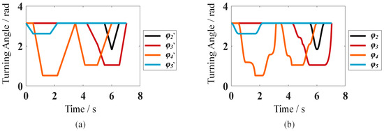
Figure 8.
Driving law of tumbling mode. (a) Driving law before planning (φ′f). (b) Driving law after planning (φf).
Based on Equations (21) and (24), the mechanical power curves of the robot under two tumbling mode driving laws can be obtained, as shown in Figure 9.
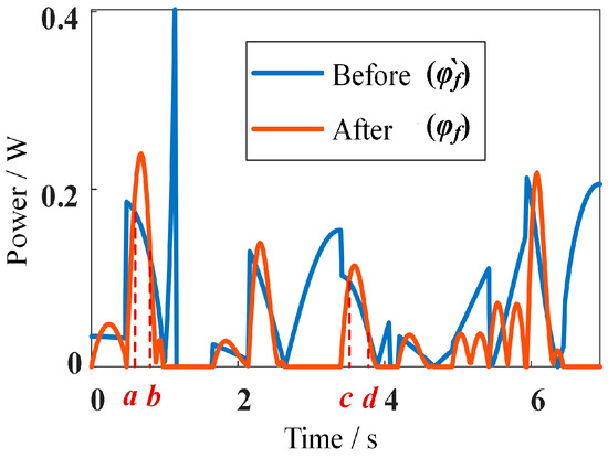
Figure 9.
The mechanical power curve of tumbling mode.
In some periods (a~b, c~d, etc., shown in Figure 9), the mechanical power is higher when the robot moves with the optimized drive law. In the case of periods a–b, the speed and torque of the body linkage are higher when it moves in a cubic curve. Still, the overall mechanical energy consumption of the robot is calculated to be reduced in this process, which is in line with reducing energy consumption. The robot moves in a tumbling mode for one cycle with a distance of 29.71 cm. By bringing the two tumbling mode driving laws into Equation (25) and calculating the mechanical energy consumption of the robot under the two tumbling mode driving laws, a graph of the energy consumption of the robot can be obtained, as shown in Figure 10.
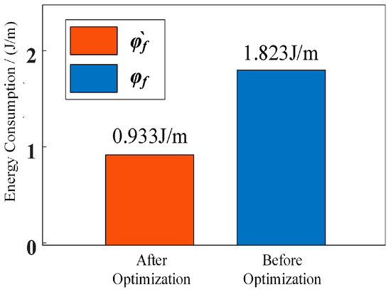
Figure 10.
The mechanical energy consumption of the tumbling mode.
It can be obtained that the energy consumption before planning is 1.823 J/m, and the mechanical energy consumption of the robot after planning is 0.933 J/m. The energy consumption ratio of the robot after planning becomes 51.16% of that before planning.
4.3. Curl–Stretch Mode
In the curl–stretch mode, the robot’s wheel-legs and body move in concert to curl and stretch, and the wheel-legs rotate in response to the body’s movement. The sequence of the robot on the flat ground is shown in Figure 11. The front wheel-legs of the robot remain relatively stationary to the ground in states 1~3, and the rear wheel-legs of the robot remain relatively stationary to the ground in states 3~5.
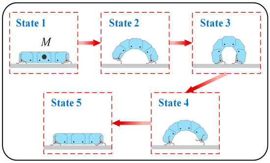
Figure 11.
Locomotion sequence of the curl–stretch mode.
According to the previous method, the driving laws before and after planning can be obtained as Equations (34) and (35). When the robot operates with these two laws, the wheel-legs rotate by 120 degrees in one cycle, and it can move to the next cycle. We take φ′q as the drive law before planning and φq as the drive law after planning.
After calculation, when 0.333 < t < 0.48, the body joint A5 can complete the subsequent transportation by gravity, and when t > 0.48, all the body joints can complete the extension movement by gravity.
Based on Equations (21), (24), (34) and (35), the mechanical power curves of the robot under two kinds of curl–stretch mode driving laws can be obtained, as shown in Figure 12.
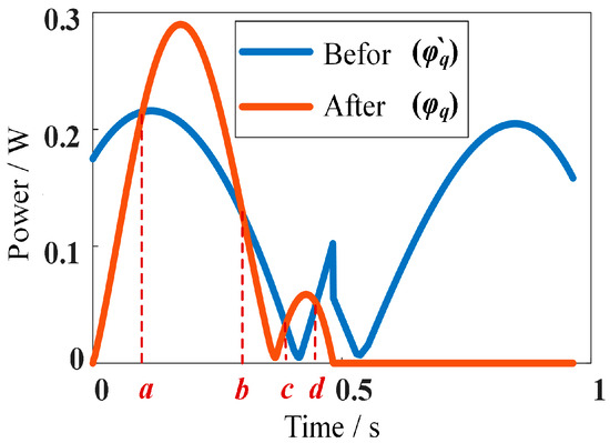
Figure 12.
Mechanical power curves of the robot’s curl–stretch mode.
It can be observed that the robot’s mechanical power is higher when it moves with the optimized drive law in periods a~b and c~d. Still, it is significantly reduced in the other periods. The robot’s distance in one curl–stretch motion cycle is 4.36 cm. By bringing Equations (34) and (35) into Equation (25) to calculate the mechanical energy consumption of the robot under the two synchronized mode drive laws, respectively, we can obtain the energy consumption of the robot, as shown in Figure 13.
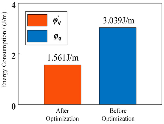
Figure 13.
Mechanical energy consumption of the robot’s curl–stretch mode.
The energy consumption of the robot before planning is 3.039 J/m and that after planning is 1.561 J/m. The energy consumption ratio after planning becomes 51.36% of that before planning.
5. Experiment
The multi-mode wheel-legged robot is constructed with a rigid structure, as shown in Figure 14. The robot’s dimensions are 14 cm × 11 cm × 3.3 cm, the body linkage is 25 mm long, and the mass is 250 g. It consists of wheel-legs made of steel splices and a robot body made of aluminum alloy. Each wheel-leg is a three-spoke wheel-leg made of four steel parts spliced together, and screws fix the four parts to the shaft of the encoder DC motor (GM12-N20VA), which is directly fixed to the body. A planar five-link structure was chosen for the robot’s body. A separate encoder DC motor drives each joint. Each motor on the body is screwed to a linkage structure, and the shaft of the motor is connected to another body linkage through a flange structure.
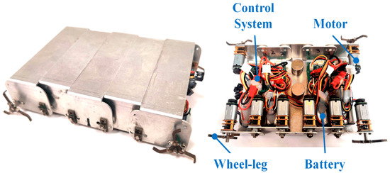
Figure 14.
A physical prototype of the mobile robot.
The robot control system comprises four controllers, each consisting of an STM32F103RCT6 chip, two DC motor drivers, and a serial converter chip. Two DC encoder motors can be controlled simultaneously on each controller. Each controller can receive external signals and start operation simultaneously through a signal receiver. Each controller collects motor torque data through the ADC sampling function of the control system and sends the data to the computer through USART. The control system framework is shown in Figure 15.
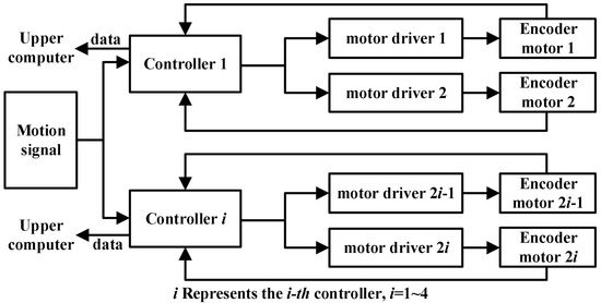
Figure 15.
Control system framework.
Because each STM32 chip is expected to be enabled with data transmission, motor motion control, and motion signal acceptance, the robot control system proposed in this paper uses the design scheme of four controllers in a distributed arrangement, as shown in Figure 16. This scheme can better utilize the chip’s computing power and save cost.
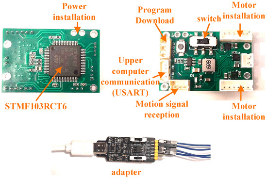
Figure 16.
Control system hardware.
To better conduct the experiment, the robot’s upper computer software was developed, and its interface is shown in Figure 17. This upper computer software can be used to adjust the robot PID parameters and can also display the robot’s energy consumption data in real time, which is convenient for operation.
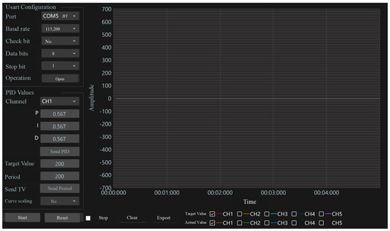
Figure 17.
Upper computer software.
During the experiment, it was found that there is friction in the motor reducer, and gravity cannot completely overcome the effect of friction during the robot’s movement. The detected driving torque τc includes the theoretical torque τi and friction torque τf, as shown in Equation (36).
Equation (37) is the Coulomb–Viscous friction model.
Measuring the robot’s torque deviation from the theoretical torque at different speeds can be solved for fa = 0.00601 and fb = 0.00579. Therefore, the theoretical torque τi can be obtained from the measurement of τc in the experiment.
Multi-locomotion experiments of the robot under different terrains were conducted, and the robot’s mechanical power data were sampled every 10 ms. Relevant video is provided in Video S1.
5.1. Flat Ground
The motion sequence diagram for one cycle of the robot’s motion on a flat surface in synchronized mode is shown in Figure 18.
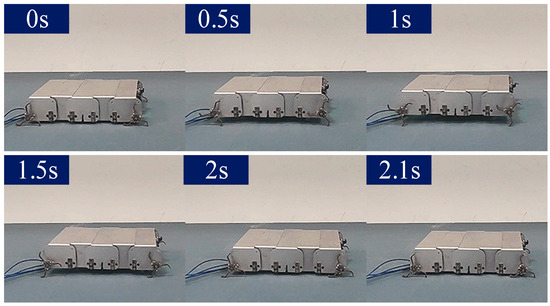
Figure 18.
Motion of the robot’s synchronized mode on flat ground.
The above robot motion was repeated five times, each with the before and after optimized driving laws, and the average distance of each cycle of the robot’s synchronized mode on the flat ground was measured to be 2.2 cm. The effect of current fluctuation was reduced by a weighted average of the five data sets, and the mechanical power of the synchronized mode on the flat ground was obtained, as shown in Figure 19.
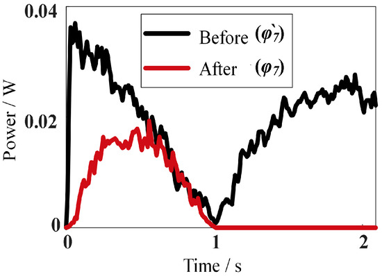
Figure 19.
Mechanical power curves of the robot’s synchronized mode on flat ground.
Compared with Figure 5, the mechanical power curve of the robot in synchronized mode has fluctuations because only 300 pulses are used for control feedback when the DC encoder motor rotates 360 degrees. The drive speed fluctuates greatly when PID feedback control is performed, but the trend in the mechanical power measured by the robot is basically the same as the theory. Based on the mechanical power curves shown in Figure 19, the mechanical energy consumption of the robot’s synchronized mode on flat ground can be obtained, as shown in Figure 20.
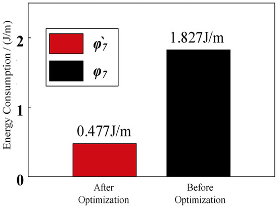
Figure 20.
Mechanical energy consumption of the robot’s synchronized mode on flat ground.
The mechanical energy consumption of the robot before planning is 0.477 J/m and 1.827 J/m, respectively, and the energy consumption after planning is 26.10% of that before planning. This is consistent with the theoretical results.
The motion sequence for one cycle of the robot on flat ground with a tumbling mode is shown in Figure 21.
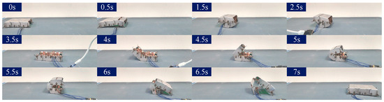
Figure 21.
Motion of the robot’s tumbling mode on flat ground.
The above robot motion was repeated five times, each with the driving law before and after planning, respectively, and the average distance moved by the robot’s tumbling mode in each cycle on the flat ground was measured to be 27.2 cm. It was found that a slide occurred during the experiment, so the actual measured value was smaller than the theoretical value. The effect of current fluctuation is reduced by a weighted average of five data sets. The mechanical power curve of the tumbling mode movement on flat ground is obtained, as shown in Figure 22.
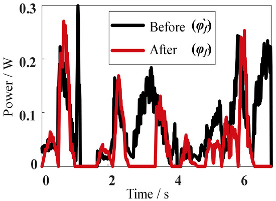
Figure 22.
Mechanical power curve of the robot’s tumbling mode on flat ground.
Compared with Figure 9, the robot’s tumbling mode’s mechanical power curve fluctuates more than the synchronized mode because the robot will collide with the ground during the tumbling motion. However, the trend in the tumbling mode’s mechanical power curve is consistent with theory. Based on the mechanical power curve shown in Figure 19, the mechanical energy consumption of the robot’s tumbling mode on flat ground shown in Figure 23 is obtained.
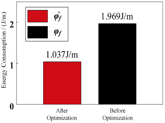
Figure 23.
Mechanical energy consumption of the robot’s tumbling mode on flat ground.
The mechanical energy consumption of the robot before planning is 1.969 J/m and 1.037 J/m, respectively, and the energy consumption after planning is 52.68% of that before planning. This is basically consistent with the theoretical results.
The motion sequence for one cycle of the robot on flat ground with a curl–stretch mode is shown in Figure 24.
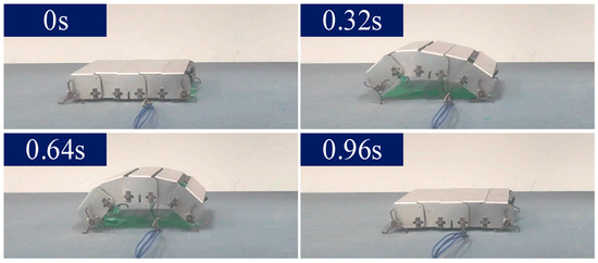
Figure 24.
Energy consumption of the robot’s curl–stretch mode on flat ground.
The above robot motions were repeated five times, each with the before and after optimized driving laws, respectively, and the average distance traveled by the robot in each cycle of the curl–stretch mode on flat ground was measured to be 4.4 cm. The effect of current fluctuation was reduced by a weighted average of the five data sets, and the mechanical power curves of the curl–stretch mode on flat ground were obtained, as shown in Figure 25.
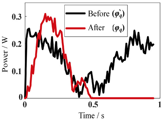
Figure 25.
Mechanical power curve of the robot’s curl–stretch mode on flat ground.
Compared with Figure 12, the power curve of the curl–stretch mode fluctuates, but the trend is basically consistent with the theory. Based on Figure 25, the mechanical energy consumption of the curl–stretch mode on flat ground, as shown in Figure 26, can be obtained.
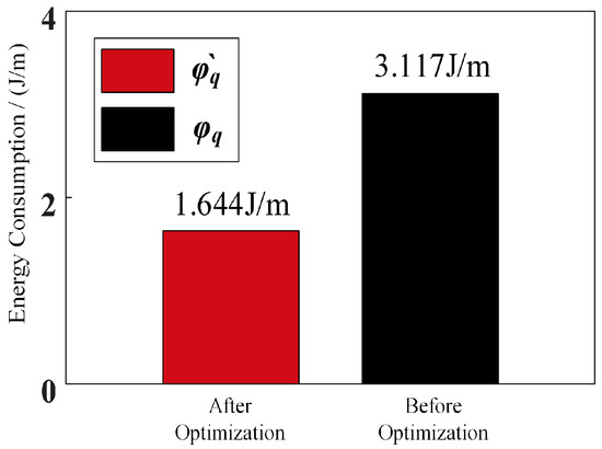
Figure 26.
Mechanical energy consumption of robot’s curl–stretch mode on flat ground.
The mechanical energy consumption of the robot before planning is 3.117 J/m and 1.644 J/m, respectively, and the energy consumption after planning is 52.73% of that before planning. This is basically consistent with the theoretical results. The above three experiments show that the robot has the lowest energy consumption when running on flat ground in synchronized mode.
5.2. Soft Ground
The motion of the robot’s synchronized mode on soft ground is shown in Figure 27.
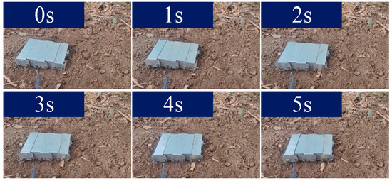
Figure 27.
Motion of the robot’s synchronized mode on soft ground.
The robot moved on the soft ground for two cycles, and the average distance moved by the robot in each cycle was measured to be 0.51 cm, which is much shorter than the distance moved by the synchronized mode on flat ground. Therefore, it is considered that the robot cannot achieve effective movement on soft ground when it relies on the wheel-leg structure.
The motion sequence of the tumbling mode on soft ground is shown in Figure 28.
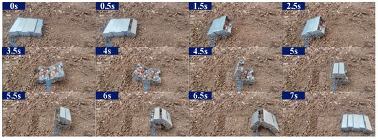
Figure 28.
Motion of the robot’s tumbling mode on soft ground.
Repeating the above process five times with the before and after optimized driving laws, we observe that the robot moves a distance of 22.1 cm in one cycle on soft ground with the tumbling mode. It is considered that the robot can achieve effective movement on soft ground. The distance traveled by the robot in tumbling mode on soft ground decreases compared with the movement on flat ground, which is caused by the fact that the soft terrain cannot provide enough friction to the robot at some moments during the movement, and the robot slips in the process of power transportation.
The mechanical power curve of the robot on soft ground is shown in Figure 29.
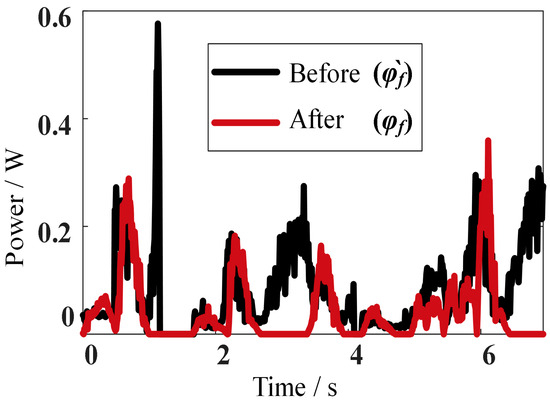
Figure 29.
Mechanical power curve of the robot’s tumbling mode on soft ground.
A comparison between Figure 29 with Figure 9 shows that the robot’s power moving on soft ground has deviation from the theoretical analysis. When the robot moves on soft ground, its position and attitude change, affecting its mechanical power. The effect of soft ground on the robot’s motion can be reduced by weighing the data from multiple experiments. The robot’s mechanical energy consumption, shown in Figure 30, is also increased compared with the motion on flat ground.
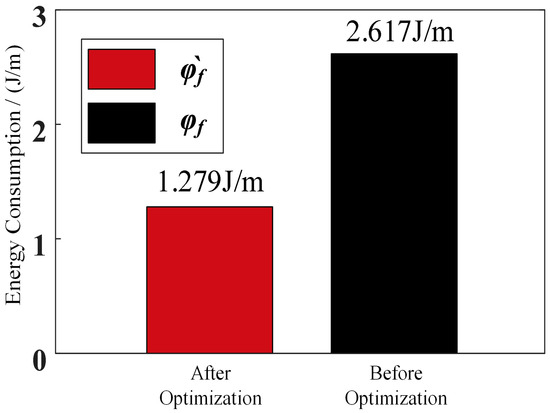
Figure 30.
Mechanical energy consumption of the robot’s tumbling mode on soft ground.
The mechanical energy consumption of the robot before planning is 2.584 J/m, and after planning, it is 1.278 J/m. The energy consumption after planning is 48.89% of that before planning. It is concluded that the planning method is still effective when applied on soft ground.
5.3. Downhill
The laws of motion for the synchronized mode and the tumbling mode planned in the previous section cannot be applied to downhill slopes, so only the curl–stretch mode is discussed. The motion sequence of the robot in the curl–stretch mode on a 30° slope is shown in Figure 31.
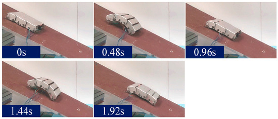
Figure 31.
Motion of the robot’s curl–stretch mode on downhill.
Repeating the above process with the before and after optimized driving laws five times, we observe that the robot moves a distance of 7.1 cm for one cycle on the downhill terrain with the curl–stretch mode. The robot slips due to friction, so the actual moving distance is larger than the theoretical distance. The mechanical power curve of the robot moving downhill is shown in Figure 32.
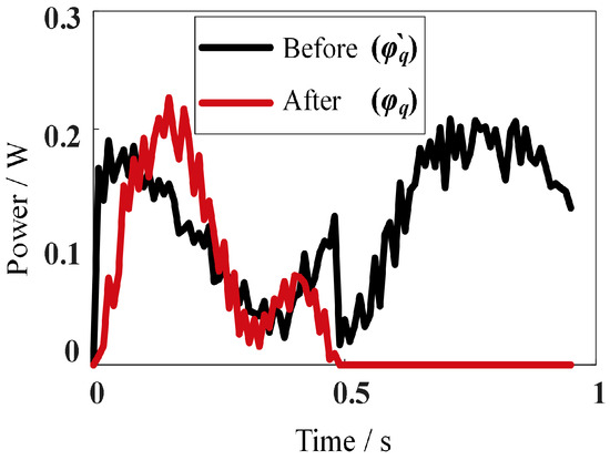
Figure 32.
Mechanical power curve of the robot’s curl–stretch mode on downhill.
Comparing Figure 32 with Figure 12, the mechanical power of the curl–stretch mode downhill has some changes compared with the robot’s motion on flat ground because the direction of movement is different from the direction of gravity the robot is subjected to. As shown in Figure 33, the mechanical energy consumption of the robot before planning is 1.659 J/m, and after planning, it is 0.655 J/m. The energy consumption after planning is 39.48% of that before planning. The mechanical energy consumption of the robot moving downhill with the curl–stretch mode is also reduced compared with the movement on flat ground. It is concluded that the planning method is still effective when applied to downhill terrain.
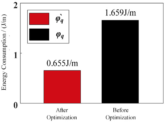
Figure 33.
Mechanical energy consumption of the robot’s curl–stretch mode on downhill.
New driving laws can further reduce the robot’s energy consumption for the curl–stretch mode on slopes. The driving laws before and after planning are shown in Equations (38) and (39), where the A5 joint moves by gravity at t > 0.33 until φ5 = 137.4°.
When the robot moves with Equations (38) and (39) as the driving law, the motion sequence of the curl–stretch mode in downhill rolling is shown in Figure 34.
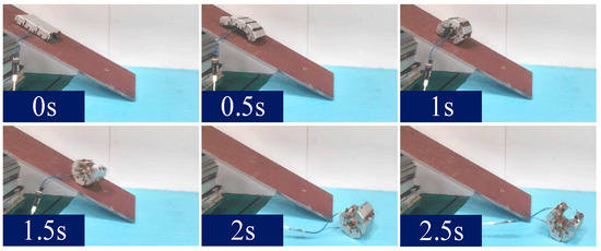
Figure 34.
Rolling of the robot’s curl–stretch mode on downhill.
Repeating the above process five times with the before and after optimized driving laws, we observe that the robot moves a distance of 61.2 cm for one cycle on the downhill terrain with the curl–stretch mode. The mechanical power curve of the robot rolling downhill is obtained, as shown in Figure 35.
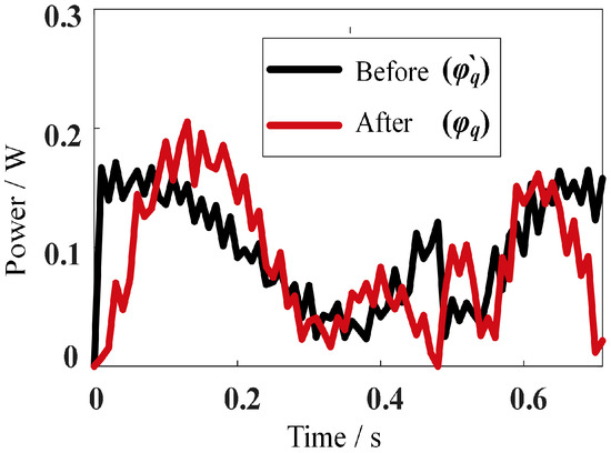
Figure 35.
The mechanical power curve of the robot’s curl–stretch mode rolling downhill.
There are some changes in the mechanical power curve shown in Figure 35 with the robot’s curl–stretch mode on flat ground. As shown in Figure 36, the mechanical energy consumption of the robot before planning is 0.114 J/m and 0.104 J/m, respectively, and after planning, it is 91.23% of that before planning. The mechanical energy consumption of the robot rolling downhill in the curl–stretch mode is reduced compared with the motion on flat ground. It is concluded that the planning method is still effective when applied to downhill terrain. The curl–stretch rolling mode has the least mechanical energy consumption when facing long downhill distances.
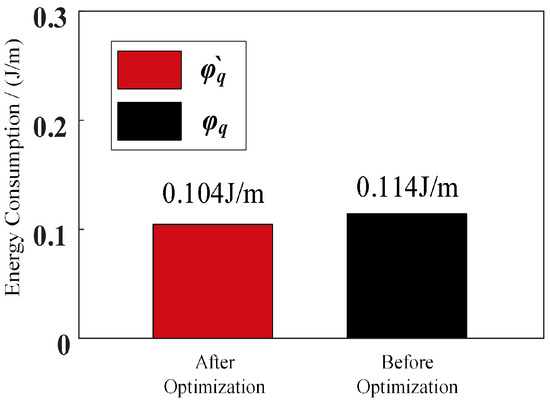
Figure 36.
Mechanical energy consumption of the robot’s curl–stretch mode rolling downhill.
6. Conclusions
In this paper, a low-energy wheel-legged mobile robot with multiple modes, including the following three kinds of modes: the synchronized mode, the tumbling mode, and the curl–stretch mode, is proposed. The kinematics and dynamics models of the robot are established, and a low-energy planning method is proposed for three typical terrains: flat ground, soft ground, and downhill terrain. The effects of the modes and driving laws on the mechanical energy consumption of the wheel-legged mobile robot in different terrains are investigated. The modes that consume the least amount of energy are obtained for the three terrains. The experimental results show that the energy consumption of the robot is significantly reduced after the planning of the driving law. Future work will focus on the robot’s autonomous mode switching planning to realize the robot’s terrain recognition and autonomous mode switching for different terrains to increase the robot’s application in more terrains.
Supplementary Materials
The following supporting information can be downloaded at: https://www.mdpi.com/article/10.3390/machines12020098/s1, Video S1: Multi-locomotion experiments of the robot under different terrains.
Author Contributions
The individual contributions of authors: conceptualization, J.L. and Y.L.; methodology, Z.Z.; software, Z.Y.; validation, Z.Z.; formal analysis, J.L.; investigation, Y.Z.; resources, J.L.; data curation, Y.G.; writing—original draft preparation, Y.L. and Z.Y.; writing—review and editing, J.L. and Z.Z.; supervision, T.S.; project administration, J.L.; funding acquisition, T.S. All authors have read and agreed to the published version of the manuscript.
Funding
This research was funded by the National Key R&D Program of China under Grant 2022YFB4701200, and the Science, Technology and Innovation Commission of Shenzhen Municipality under Grant ZDSYS20220527171403009 and JCYJ20220818100417038.
Data Availability Statement
Data are contained within the article.
Acknowledgments
The authors are grateful to the Mechanisms and Robotic System Laboratory of Tianjin University and the Centre for Advanced Mechanisms and Robotics of Tianjin University for providing this research opportunity and financial support.
Conflicts of Interest
The authors declare no conflicts of interest.
References
- Wang, K.; Sun, Z.; Nishimori, T.; Li, Z. Research on Current Situation and Trend of Robot Education in Japan. Mod. Educ. Technol. 2017, 27, 5–11. [Google Scholar]
- Smith, J.A.; Jivraj, J.; Wong, R.; Yang, V. 30 years of neurosurgical robots: Review and trends for manipulators and associated navigational systems. Ann. Biomed. Eng. 2016, 44, 836–846. [Google Scholar] [CrossRef]
- Zhu, Y.; Fei, Y.; Xu, H. Stability analysis of a wheel-track-leg hybrid mobile robot. J. Intell. Robot. Syst. 2018, 91, 515–528. [Google Scholar] [CrossRef]
- Liu, J.; Zhan, J.; Guo, C.; Li, Y.; Wu, H.; Huang, H. Data logic structure and key technologies on intelligent high-precision map. J. Geod. Geoinf. Sci. 2020, 3, 1–17. [Google Scholar]
- Xie, Y.; Zhang, X.; Meng, W.; Zheng, S.; Jiang, L.; Meng, J.; Wang, S. Coupled fractional-order sliding mode control and obstacle avoidance of a four-wheeled steerable mobile robot. ISA Trans. 2021, 108, 282–294. [Google Scholar] [CrossRef] [PubMed]
- Drotman, D.; Jadhav, S.; Sharp, D.; Chan, C.; Tolley, M.T. Electronics-free pneumatic circuits for controlling soft-legged robots. Sci. Robot. 2021, 6, eaay2627. [Google Scholar] [CrossRef] [PubMed]
- Dang, T.; Tranzatto, M.; Khattak, S.; Mascarich, F.; Alexis, K.; Hutter, M. Graph-based subterranean exploration path planning using aerial and legged robots. J. Field Robot. 2020, 37, 1363–1388. [Google Scholar] [CrossRef]
- Picardi, G.; Chellapurath, M.; Iacoponi, S.; Stefanni, S.; Laschi, C.; Calisti, M. Bioinspired underwater legged robot for seabed exploration with low environmental disturbance. Sci. Robot. 2020, 5, eaaz1012. [Google Scholar] [CrossRef] [PubMed]
- Huang, Z.; Bauer, R.; Pan, Y.-J. Event-triggered formation tracking control with application to multiple mobile robots. IEEE Trans. Ind. Electron. 2022, 70, 846–854. [Google Scholar] [CrossRef]
- Xu, S.; Peng, H. Design, analysis, and experiments of preview path tracking control for autonomous vehicles. IEEE Trans. Intell. Transp. Syst. 2019, 21, 48–58. [Google Scholar] [CrossRef]
- Velimirovic, A.; Velimirovic, M.; Hugel, V.; Iles, A.; Blazevic, P. A new architecture of robot with “wheels-with-legs” (WWL). In Proceedings of the AMC’98-Coimbra. 1998 5th International Workshop on Advanced Motion Control. Proceedings (Cat. No. 98TH8354), Coimbra, Portugal, 29 June–1 July 1998; pp. 434–439. [Google Scholar]
- Zhang, H.; Zhang, X.; Huang, Y.; Du, J.; Zhu, B. A novel reconfigurable wheel-legged mobile mechanism. In Proceedings of the International Design Engineering Technical Conferences and Computers and Information in Engineering Conference, Los Angeles, CA, USA, 18–21 August 2019; p. V05AT07A011. [Google Scholar]
- Chen, W.-H.; Lin, H.-S.; Lin, Y.-M.; Lin, P.-C. TurboQuad: A novel leg–wheel transformable robot with smooth and fast behavioral transitions. IEEE Trans. Robot. 2017, 33, 1025–1040. [Google Scholar] [CrossRef]
- Wang, S.; Chen, Z.; Li, J.; Wang, J.; Li, J.; Zhao, J. Flexible motion framework of the six wheel-legged robot: Experimental results. IEEE/ASME Trans. Mechatron. 2021, 27, 2246–2257. [Google Scholar] [CrossRef]
- Chen, Z.; Wang, S.; Wang, J.; Xu, K.; Lei, T.; Zhang, H.; Wang, X.; Liu, D.; Si, J. Control strategy of stable walking for a hexapod wheel-legged robot. ISA Trans. 2021, 108, 367–380. [Google Scholar] [CrossRef] [PubMed]
- Huang, J.; Wang, Y.; Fang, C.; Yi, M.; Lan, G. Walking Efficiency and Crossing Obstacle Ability of Variable Eccentric Wheel-legged Robot. In Proceedings of the Advances in Materials, Machinery, Electrical Engineering (AMMEE 2017), Tianjin, China, 10–11 June 2017; pp. 298–304. [Google Scholar]
- Smith, L.M.; Quinn, R.D.; Johnson, K.A.; Tuck, W.R. The Tri-Wheel: A novel wheel-leg mobility concept. In Proceedings of the 2015 IEEE/RSJ International Conference on Intelligent Robots and Systems (IROS), Hamburg, Germany, 28 September–2 October 2015; pp. 4146–4152. [Google Scholar]
- Saranli, U.; Buehler, M.; Koditschek, D.E. RHex: A simple and highly mobile hexapod robot. Int. J. Robot. Res. 2001, 20, 616–631. [Google Scholar] [CrossRef]
- Komsuoglu, H.; McMordie, D.; Saranli, U.; Moore, N.; Buehler, M.; Koditschek, D.E. Proprioception based behavioral advances in a hexapod robot. In Proceedings of the 2001 ICRA. IEEE International Conference on Robotics and Automation (Cat. No. 01CH37164), Seoul, Republic of Korea, 21–26 May 2001; pp. 3650–3655. [Google Scholar]
- Saranli, U.; Koditschek, D.E. Back flips with a hexapedal robot. In Proceedings of the 2002 IEEE International Conference on Robotics and Automation (Cat. No. 02CH37292), Washington, DC, USA, 11–15 May 2002; pp. 2209–2215. [Google Scholar]
- Saranli, U.; Koditschek, D.E. Template based control of hexapedal running. In Proceedings of the 2003 IEEE International Conference on Robotics and Automation (Cat. No. 03CH37422), Taipei, Taiwan, 14–19 September 2003; pp. 1374–1379. [Google Scholar]
- Saranli, U.; Rizzi, A.A.; Koditschek, D.E. Model-based dynamic self-righting maneuvers for a hexapedal robot. Int. J. Robot. Res. 2004, 23, 903–918. [Google Scholar] [CrossRef]
- Greenfield, A.; Saranli, U.; Rizzi, A.A. Solving models of controlled dynamic planar rigid-body systems with frictional contact. Int. J. Robot. Res. 2005, 24, 911–931. [Google Scholar] [CrossRef]
- Lin, Y.; Tian, Y.; Xue, Y.; Han, S.; Zhang, H.; Lai, W.; Xiao, X. Innovative design and simulation of a transformable robot with flexibility and versatility, RHex-T3. In Proceedings of the 2021 IEEE International Conference on Robotics and Automation (ICRA), Xi’an, China, 30 May–5 June 2021; pp. 6992–6998. [Google Scholar]
- Sun, C.; Yang, G.; Yao, S.; Liu, Q.; Wang, J.; Xiao, X. RHex-T3: A Transformable Hexapod Robot with Ladder Climbing Function. IEEE/ASME Trans. Mechatron. 2023, 28, 1939–1947. [Google Scholar] [CrossRef]
- Quinn, R.D.; Offi, J.T.; Kingsley, D.A.; Ritzmann, R.E. Improved mobility through abstracted biological principles. In Proceedings of the IEEE/RSJ International Conference on Intelligent Robots and Systems, Lausanne, Switzerland, 30 September–4 October 2002; pp. 2652–2657. [Google Scholar]
- Allen, T.J.; Quinn, R.D.; Bachmann, R.J.; Ritzmann, R.E. Abstracted biological principles applied with reduced actuation improve mobility of legged vehicles. In Proceedings of the 2003 IEEE/RSJ International Conference on Intelligent Robots and Systems (IROS 2003) (Cat. No. 03CH37453), Las Vegas, NV, USA, 27–31 October 2003; pp. 1370–1375. [Google Scholar]
- Schroer, R.T.; Boggess, M.J.; Bachmann, R.J.; Quinn, R.D.; Ritzmann, R.E. Comparing cockroach and Whegs robot body motions. In Proceedings of the IEEE International Conference on Robotics and Automation, 2004. Proceedings. ICRA’04. 2004, New Orleans, LA, USA, 26 April–1 May 2004; pp. 3288–3293. [Google Scholar]
- Daltorio, K.A.; Horchler, A.D.; Gorb, S.; Ritzmann, R.E.; Quinn, R.D. A small wall-walking robot with compliant, adhesive feet. In Proceedings of the 2005 IEEE/RSJ international conference on intelligent robots and systems, Edmonton, AB, Canada, 2–6 August 2005; pp. 3648–3653. [Google Scholar]
- Breckwoldt, W.; Bachmann, R.; Leibach, R.; Quinn, R. Speedy whegs climbs obstacles slowly and runs at 44 km/hour. In Proceedings of the Biomimetic and Biohybrid Systems: 8th International Conference, Living Machines 2019, Nara, Japan, 9–12 July 2019; Proceedings 8. pp. 27–37. [Google Scholar]
- Gyarmati, M.; Kadar, F.; Horea, G.; Tătar, M.O. Contributions to the Search and Rescue Robots’development with Tristar and Whegs Units. Acta Tech. Napoc. Ser. Appl. Math. Mech. Eng. 2022, 65. [Google Scholar]
- Eich, M.; Grimminger, F.; Bosse, S.; Spenneberg, D.; Kirchner, F. Asguard: A hybrid legged wheel security and sar-robot using bio-inspired locomotion for rough terrain. In Proceedings of the IARP/EURON Workshop on Robotics for Risky Interventions and Enviromental Surveillance, Benicàssim, Spain, 7–8 January 2008. [Google Scholar]
- Wilcox, B.H.; Litwin, T.; Biesiadecki, J.; Matthews, J.; Heverly, M.; Morrison, J.; Townsend, J.; Ahmad, N.; Sirota, A.; Cooper, B. ATHLETE: A cargo handling and manipulation robot for the moon. J. Field Robot. 2007, 24, 421–434. [Google Scholar] [CrossRef]
- Smith, J.A.; Sharf, I.; Trentini, M. PAW: A hybrid wheeled-leg robot. In Proceedings of the 2006 IEEE International Conference on Robotics and Automation, ICRA 2006, Orlando, FL, USA, 15–19 May 2006; pp. 4043–4048. [Google Scholar]
- Luo, Y.; Li, Q.; Liu, Z. Design and optimization of wheel-legged robot: Rolling-Wolf. Chin. J. Mech. Eng. 2014, 27, 1133–1142. [Google Scholar] [CrossRef]
- Sun, T.; Yang, S.-F.; Huang, T.; Dai, J.S. A finite and instantaneous screw based approach for topology design and kinematic analysis of 5-axis parallel kinematic machines. Chin. J. Mech. Eng. 2018, 31, 44. [Google Scholar] [CrossRef]
- Yang, C.; Geng, S.; Walker, I.; Branson, D.T.; Liu, J.; Dai, J.S.; Kang, R. Geometric constraint-based modeling and analysis of a novel continuum robot with shape memory alloy initiated variable stiffness. Int. J. Robot. Res. 2020, 39, 1620–1634. [Google Scholar] [CrossRef]
- Li, J.; Liu, Y.; Yu, Z.; Guan, Y.; Zhao, Y.; Zhuang, Z.; Sun, T. Design, Analysis, and Experiment of a Wheel-Legged Mobile Robot. Appl. Sci. 2023, 13, 9936. [Google Scholar] [CrossRef]
Disclaimer/Publisher’s Note: The statements, opinions and data contained in all publications are solely those of the individual author(s) and contributor(s) and not of MDPI and/or the editor(s). MDPI and/or the editor(s) disclaim responsibility for any injury to people or property resulting from any ideas, methods, instructions or products referred to in the content. |
© 2024 by the authors. Licensee MDPI, Basel, Switzerland. This article is an open access article distributed under the terms and conditions of the Creative Commons Attribution (CC BY) license (https://creativecommons.org/licenses/by/4.0/).