


Realization of a Human-like Gait for a Bipedal Robot Based on Gait Analysis †

Abstract
1. Introduction
2. Materials and Methods
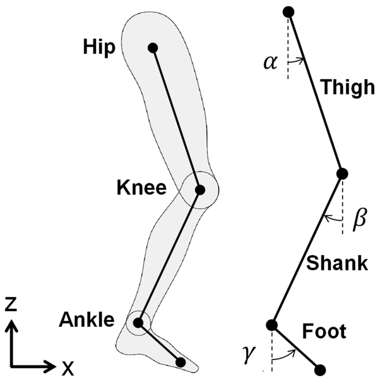
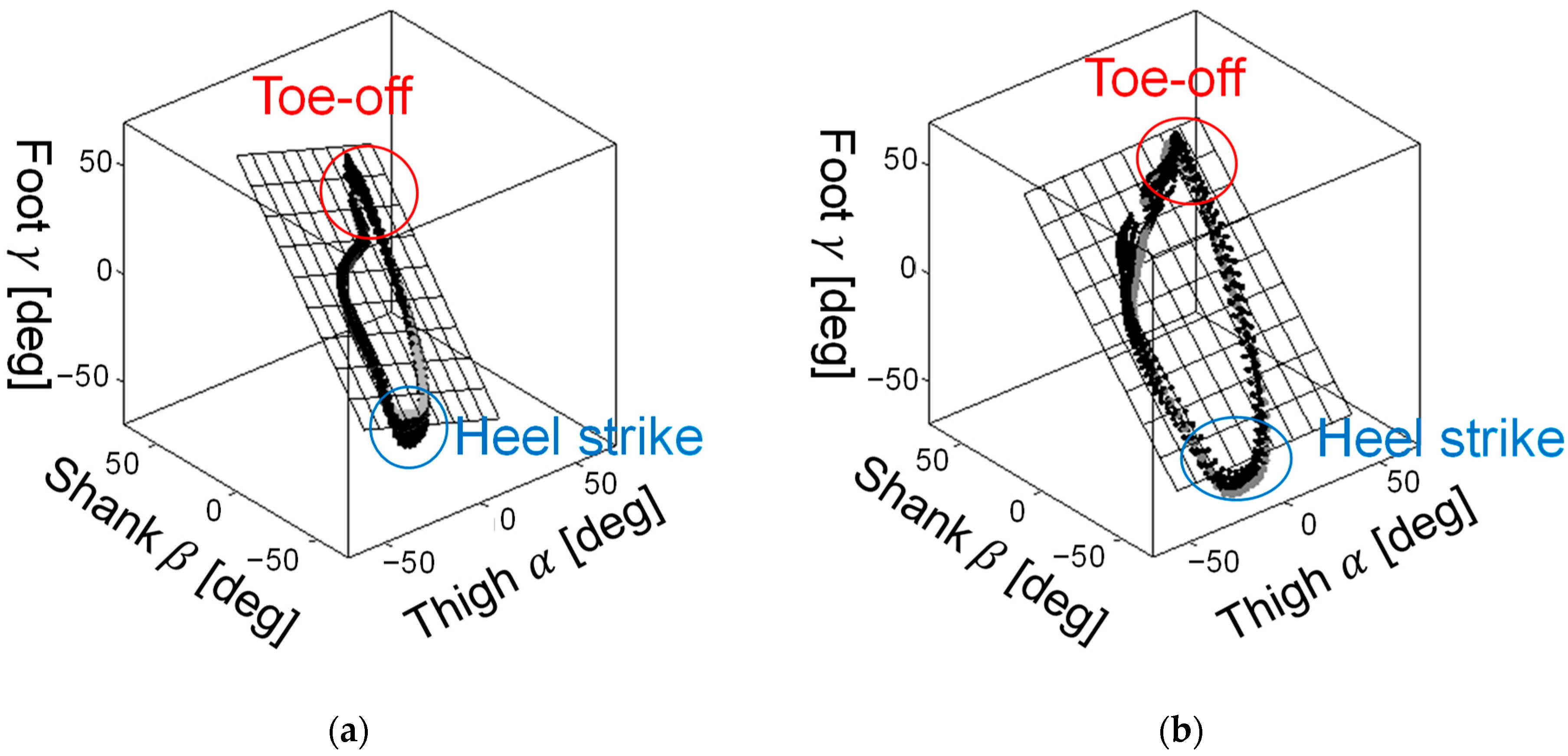
2.1. Characteristics of the Human Gait
2.2. Simulation Environment
2.3. Control Method
2.3.1. Deep Reinforcement Learning
2.3.2. Policy Gradient Methods
2.3.3. Neural Network
2.3.4. Probabilistic Policy with the Gaussian Model
2.3.5. Rewards
3. Results
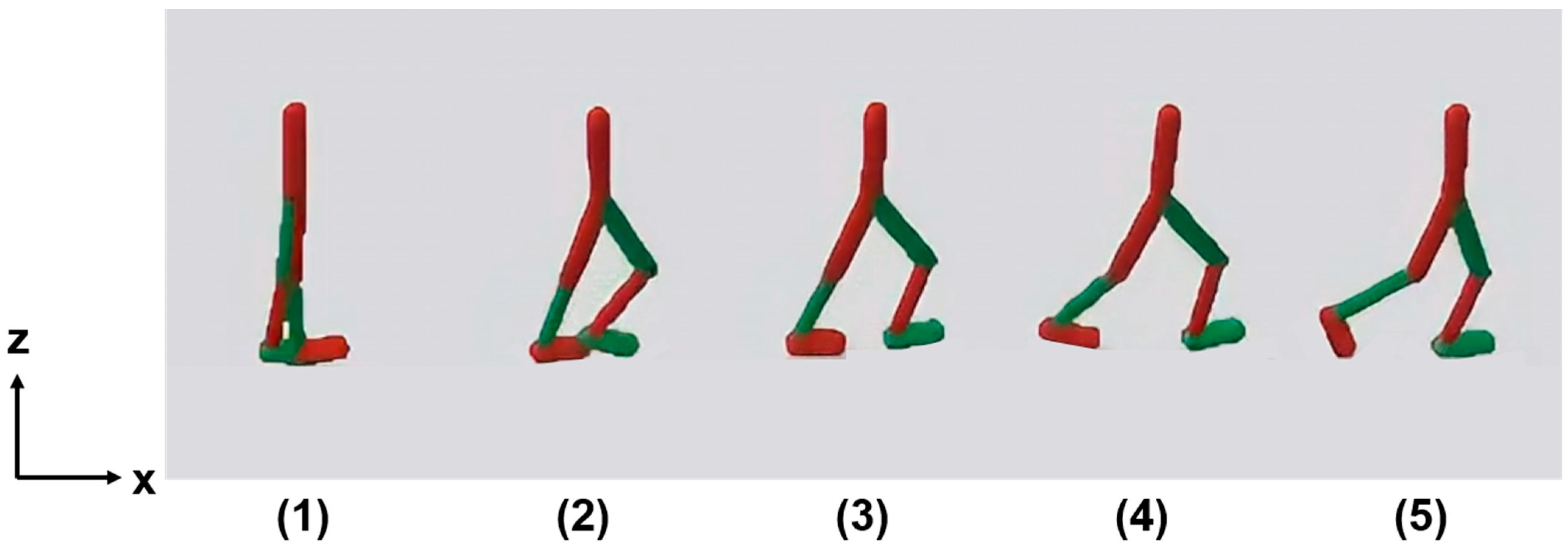
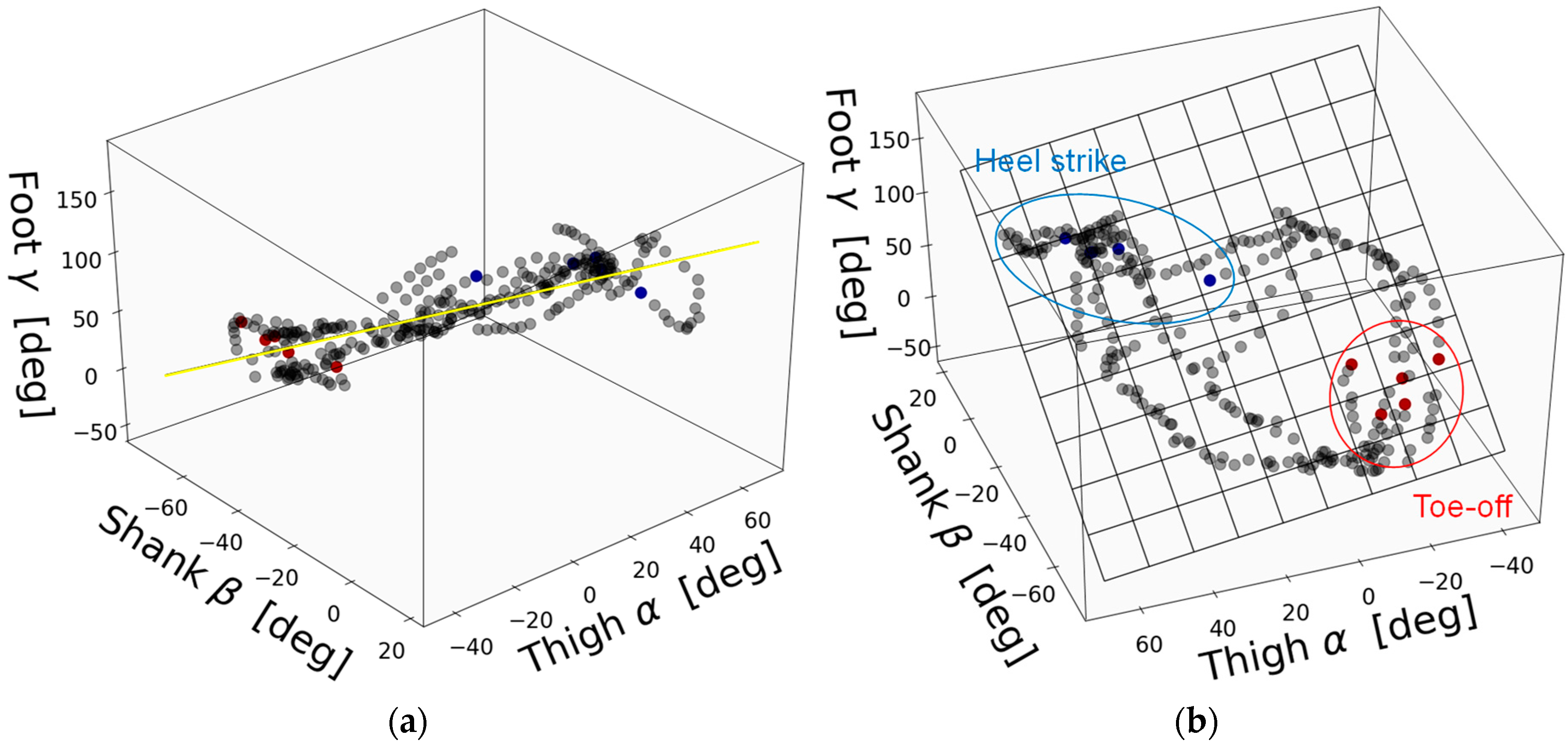
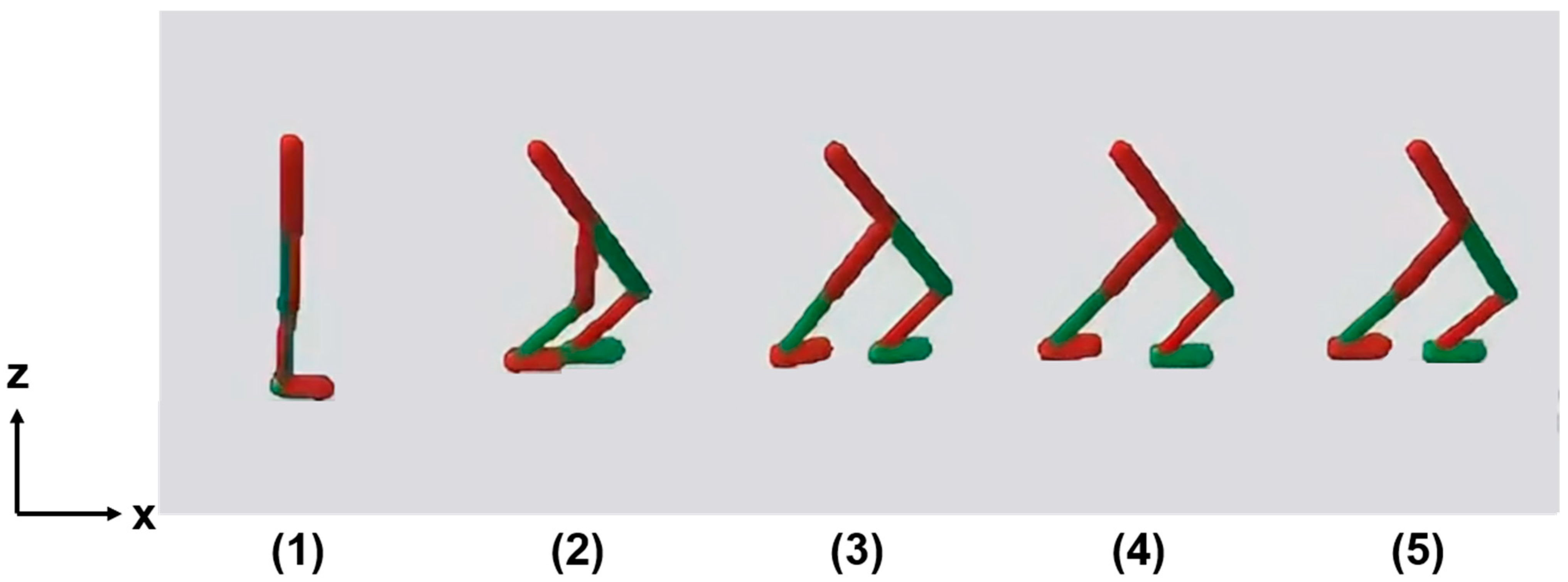
3.1. Walking Motion
3.1.1. Proposed Method
3.1.2. Comparative Method
3.2. Learning Curve
4. Discussion and Future Work
Author Contributions
Funding
Data Availability Statement
Acknowledgments
Conflicts of Interest
References
- Tomomitsu, M.S.V.; Alonso, A.C.; Morimoto, E.; Bobbio, T.G.; Greve, J.M.D. Static and dynamic postural control in low-vision and normal-vision adults. Clinics 2013, 68, 517–521. [Google Scholar] [CrossRef] [PubMed]
- Pozzo, T.; Berthoz, A.; Lefort, L. Head stabilization during various locomotor tasks in humans. Exp. Brain Res. 1990, 82, 97–106. [Google Scholar] [CrossRef]
- Venkadesan, M.; Yawar, A.; Eng, C.M.; Dias, M.A.; Singh, D.K.; Tommasini, S.M.; Haims, A.H.; Bandi, M.M.; Mandre, S. Stiffness of the human foot and evolution of the transverse arch. Nature 2020, 579, 97–100. [Google Scholar] [CrossRef] [PubMed]
- Bohm, S.; Mersmann, F.; Santuz, A.; Schroll, A.; Arampatzis, A. Muscle-specific economy of force generation and efficiency of work production during human running. eLife 2021, 10, e67182. [Google Scholar] [CrossRef] [PubMed]
- Kamikawa, Y.; Maeno, T. Underactuated Five-Finger Prosthetic Hand Inspired by Grasping Force Distribution of Humans. In Proceedings of the 2008 IEEE/RSJ International Conference on Intelligent Robots and Systems (IROS), Nice, France, 22–26 September 2008; pp. 717–722. [Google Scholar]
- Ogura, Y.; Aikawa, H.; Shimomura, K.; Morishima, A.; Lim, H.O.; Takanishi, A. Development of a New Humanoid Robot WABIAN-2. In Proceedings of the 2006 IEEE International Conference on Robotics and Automation (ICRA), Orlando, FL, USA, 15–19 May 2006; pp. 76–81. [Google Scholar]
- Hashimoto, K.; Takezaki, Y.; Hattori, K.; Kondo, H.; Takashima, T.; Lim, H.O.; Takanishi, A. A Study of Function of Foot’s Medial Longitudinal Arch Using Biped Humanoid Robot. In Proceedings of the 2010 IEEE/RSJ International Conference on Intelligent Robots and Systems (IROS), Taipei, Taiwan, 18–22 October 2010; pp. 2206–2211. [Google Scholar]
- Hashimoto, K.; Takezaki, Y.; Motohashi, H.; Otani, T.; Kishi, T.; Lim, H.O.; Takanishi, A. Biped Walking Stabilization Based on Gait Analysis. In Proceedings of the 2012 IEEE International Conference on Robotics and Automation (ICRA), Saint Paul, MN, USA, 14–18 May 2012; pp. 154–159. [Google Scholar]
- Cheng, G.; Hyon, S.H.; Morimoto, J.; Ude, A.; Colvin, G.; Scroggin, W.; Jacobsen, S.C. CB: A Humanoid Research Platform for Exploring NeuroScience. In Proceedings of the 6th IEEE-RAS International Conference on Humanoid Robots, Genova, Italy, 4–6 December 2006; pp. 182–187. [Google Scholar]
- Ude, A.; Wyar, V.; Lin, L.H.; Cheng, G. Distributed Visual Attention on a Humanoid Robot. In Proceedings of the 5th IEEE-RAS International Conference on Humanoid Robots, Tsukuba, Japan, 5 December 2005; pp. 381–386. [Google Scholar]
- Endo, N.; Takanishi, A. Development of whole-body emotional expression humanoid robot for ADL-assistive RT services. J. Robot. Mechatron. 2011, 23, 969–977. [Google Scholar] [CrossRef]
- Kryczka, P.; Falotico, E.; Hashimoto, K.; Lim, H.O.; Takanishi, A.; Laschi, C.; Dario, P.; Berthoz, A. A Robotic Implementation of a Bio-Inspired Head Motion Stabilization Model on a Humanoid Platform. In Proceedings of the 2012 IEEE/RSJ International Conference on Intelligent Robots and Systems (IROS), Vilamoura-Algarve, Portugal, 7–12 October 2012; pp. 2076–2081. [Google Scholar]
- Ferreira, J.P.; Crisóstomo, M.M.; Coimbra, A.P. Human Gait Acquisition and Characterization. IEEE Trans. Instrum. Meas. 2009, 58, 2979–2988. [Google Scholar] [CrossRef]
- Yamano, J.; Kurokawa, M.; Sakai, Y.; Hashimoto, K. Walking Motion Generation of Bipedal Robot Based on Planar Covariation Using Deep Reinforcement Learning. In Proceedings of the 26th International Conference on Climbing and Walking Robots (CLAWAR 2023), Florianópolis, Brazil, 2–4 October 2023. [Google Scholar]
- Borghese, N.A.; Bianchi, L.; Lacquaniti, F. Kinematic determinants of human locomotion. J. Physiol. 1996, 494, 863–879. [Google Scholar] [CrossRef] [PubMed]
- Ivanenko, Y.P.; d’Avella, A.; Poppele, R.E.; Lacquaniti, F. On the Origin of Planar Covariation of Elevation Angles During Human Locomotion. J. Neurophysiol. 2008, 99, 1890–1898. [Google Scholar] [CrossRef] [PubMed]
- Ogihara, N.; Kikuchi, T.; Ishiguro, Y.; Makishima, H.; Nakatsukasa, M. Planar covariation of limb elevation angles during bipedal walking in the Japanese macaque. J. R. Soc. Interface 2012, 9, 2181–2190. [Google Scholar] [CrossRef] [PubMed]
- Ha, S.S.; Yu, J.H.; Han, Y.J.; Hahn, H.S. Natural Gait Generation of Biped Robot based on Analysis of Human’s Gait. In Proceedings of the 2008 International Conference on Smart Manufacturing Application, Goyangi, Republic of Korea, 9–11 April 2008; pp. 30–34. [Google Scholar]
- Ghiasi, A.R.; Alizadeh, G.; Mirzaei, M. Simultaneous design of optimal gait pattern and controller for a bipedal robot. Multibody Syst. Dyn. 2010, 23, 410–429. [Google Scholar] [CrossRef]
- GitHub Benelot/Pybullet-Gym. Available online: https://github.com/benelot/pybullet-gym (accessed on 8 December 2023).
- PyBllet. Available online: https://pybullet.org/wordpress/ (accessed on 8 December 2023).
- Kapandji, A.I.; Owerko, C. The Physiology of the Joints: 2 The Lower Limb, 7th ed.; Handspring Publishing Limited: London, UK, 2019. [Google Scholar]
- Wang, S.; Chaovalitwongse, W.; Babuska, R. Machine learning algorithms in bipedal robot control. IEEE Trans. Syst. Man Cybern. Part C (Appl. Rev.) 2012, 42, 728–743. [Google Scholar] [CrossRef]
- Xie, Z.; Berseth, G.; Clary, P.; Hurst, J.; van de Panne, M. Feedback Control For Cassie With Deep Reinforcement Learning. In Proceedings of the 2018 IEEE/RSJ International Conference on Intelligent Robots and Systems (IROS), Madrid, Spain, 1–5 October 2018; pp. 1241–1246. [Google Scholar]
- Tsounis, V.; Alge, M.; Lee, J.; Farshidian, F.; Hutter, M. DeepGait: Planning and Control of Quadrupedal Gaits Using Deep Reinforcement Learning. IEEE Robot. Autom. Lett. 2020, 5, 3699–3706. [Google Scholar] [CrossRef]
- Wang, Z.; Wei, W.; Xie, A.; Zhang, Y.; Wu, J.; Zhu, Q. Hybrid Bipedal Locomotion Based on Reinforcement Learning and Heuristics. Micromachines 2022, 13, 1688. [Google Scholar] [CrossRef]
- Adolph, K.E.; Bertenthal, B.I.; Boker, S.M.; Goldfield, E.C.; Gibson, E.J. Learning in the Development of Infant Locomotion. Monogr. Soc. Res. Child Dev. 1997, 62, 1–140. [Google Scholar] [CrossRef]
- Abiodun, O.I.; Jantan, A.; Omolara, A.E.; Dada, K.V.; Mohamed, N.A.; Arshad, H. State-of-the-art in artificial neural network applications: A survey. Heliyon 2018, 4, e00938. [Google Scholar] [CrossRef] [PubMed]
- Sutton, R.S.; Barto, A.G. Reinforcement Learning, 2nd ed.; The MIT Press: Cambridge, MA, USA, 2018. [Google Scholar]
- Sutton, R.S.; McAllester, S.; Singh, S.; Mansour, Y. Policy gradient methods for reinforcement learning with function approximation. In Proceedings of the 12th International Conference on Neural Information Processing Systems, Denver, CO, USA, 29 November–4 December 1999. [Google Scholar]
- Castermans, T.; Duvinage, M.; Cheron, G.; Dutoit, T. Towards Effective Non-Invasive Brain-Computer Interfaces Dedicated to Gait Rehabilitation Systems. Brain Sci. 2014, 4, 1–48. [Google Scholar] [CrossRef]


| Surface | 1st | 2nd | 3rd |
|---|---|---|---|
| Hard | 77.4% | 22.0% | 0.6% |
| Soft | 72.0% | 27.4% | 0.6% |
| Joint Name | Angle [deg] |
|---|---|
| Hip Joint | −20~135 |
| Knee Joint | −140~0 |
| Ankle Joint | −45~25 |
| Layer | Detail | Dimension |
|---|---|---|
| Input | Body position | 3 |
| Body velocity | 3 | |
| Body posture | 2 | |
| Joint angle | 6 | |
| Joint angular velocity | 6 | |
| Foot ground state | 2 | |
| Hidden | Layer 1 | 220 |
| Layer 2 | 114 | |
| Layer 3 | 60 | |
| Output | Mean | 6 |
| Variance | 6 |
| Layer | Detail | Dimension |
|---|---|---|
| Input | Body position | 3 |
| Body velocity | 3 | |
| Body posture | 2 | |
| Joint angle | 6 | |
| Joint angular velocity | 6 | |
| Foot ground state | 2 | |
| Hidden | Layer 1 | 220 |
| Layer 2 | 33 | |
| Layer 3 | 5 | |
| Output | State value function | 1 |
| Leg | 1st | 2nd | 3rd |
|---|---|---|---|
| Left | 70.0% | 27.1% | 2.9% |
| Right | 72.8% | 24.0% | 3.2% |
| Leg | 1st | 2nd | 3rd |
|---|---|---|---|
| Left | 64.9% | 33.3% | 1.8% |
| Right | 78.8% | 17.8% | 3.4% |
Disclaimer/Publisher’s Note: The statements, opinions and data contained in all publications are solely those of the individual author(s) and contributor(s) and not of MDPI and/or the editor(s). MDPI and/or the editor(s) disclaim responsibility for any injury to people or property resulting from any ideas, methods, instructions or products referred to in the content. |
© 2024 by the authors. Licensee MDPI, Basel, Switzerland. This article is an open access article distributed under the terms and conditions of the Creative Commons Attribution (CC BY) license (https://creativecommons.org/licenses/by/4.0/).
Share and Cite
Yamano, J.; Kurokawa, M.; Sakai, Y.; Hashimoto, K. Realization of a Human-like Gait for a Bipedal Robot Based on Gait Analysis. Machines 2024, 12, 92. https://doi.org/10.3390/machines12020092
Yamano J, Kurokawa M, Sakai Y, Hashimoto K. Realization of a Human-like Gait for a Bipedal Robot Based on Gait Analysis. Machines. 2024; 12(2):92. https://doi.org/10.3390/machines12020092
Chicago/Turabian StyleYamano, Junsei, Masaki Kurokawa, Yuki Sakai, and Kenji Hashimoto. 2024. "Realization of a Human-like Gait for a Bipedal Robot Based on Gait Analysis" Machines 12, no. 2: 92. https://doi.org/10.3390/machines12020092
APA StyleYamano, J., Kurokawa, M., Sakai, Y., & Hashimoto, K. (2024). Realization of a Human-like Gait for a Bipedal Robot Based on Gait Analysis. Machines, 12(2), 92. https://doi.org/10.3390/machines12020092