Research on Grinding Force Prediction of Flexible Abrasive Disc Grinding Process of TC17 Titanium Alloy

Abstract

Abrasive disc grinding is currently a key manufacturing process to achieve better accuracy and high-quality surfaces of TC17 components. Grinding force, which results from the friction and elastic–plastic deformation during the contact and interaction between the abrasive grains and the workpiece, is a critical parameter that represents the grinding accuracy and efficiency. In order to understand the influence factors of grinding force, the characteristics of the flexible abrasive disc grinding process were studied. Considering the contact state between the abrasive tool and the workpiece, the theoretical model of normal grinding force was established in detail, from macro- and micro-perspectives. By conducting single-factor and orthogonal grinding experiments of TC17 components, the influence of different process parameters on the normal grinding force was revealed. The normal grinding force prediction models of the abrasive disc grinding process were developed based on the Box–Behnken design (BBD) and particle swarm optimization–back propagation (PSO-BP) neural networks, respectively. The results showed that the normal grinding force was negatively correlated with the disc rotational speed, and positively correlated with the contact angle, grinding depth, and feed rate, and the interaction of the factor feed rate and grinding depth was the more influential factor. Both the BBD and PSO-BP force models had good reliability and accuracy, and the mean absolute error (MAE) and mean relative error (MRE) of the above two prediction models were 0.22 N and 0.16 N, and 13.3% and 10.9%, respectively.

1. Introduction

Titanium alloys are widely used in various fields, such as aviation, aerospace, energy, navigation, biology, medicine, vehicles, and chemistry, due to their excellent physical and mechanical properties [1,2,3]. In particular, TC17 titanium alloy, whose main composition is Ti-5Al-2Sn-2Zr-4Mn-4Cr, has several advantages, such as high strength, hardenability, good fracture toughness, and a wide forging temperature range. Therefore, it is considered an advantageous material to meet the requirements of high structural efficiency, high reliability, and low-cost manufacturing in the field of aero-engine components.

Abrasive disc grinding is currently a key manufacturing process used to grind TC17 aero-engine blades with free-form surfaces to achieve better accuracy and high-quality surfaces [4,5]. However, due to chip deformation, cold hardening, active chemistry, and poor thermal conductivity, TC17 is recognized as a typical difficult-to-cut material. Therefore, elucidating the mechanism of the flexible grinding process of TC17 parts remains a challenge [6].

It is widely acknowledged that the grinding force is a result of the friction and elastic–plastic deformation that occurs during the contact and interaction between the abrasive and the workpiece. It is a critical parameter that represents the grinding accuracy and efficiency. Monitoring and controlling the grinding force plays a crucial role in preventing tool wear, improving the grinding efficiency, ensuring workpiece quality, and optimizing the grinding process. Excessive grinding force can lead to workpiece damage, tool life decrease, and surface quality reduction. Conversely, too little grinding force can result in an insufficient material removal rate and a low grinding efficiency. To ensure the machining quality and efficiency, it is essential to study the variation of grinding force and its influencing factors during flexible grinding contact [7].

In recent years, several studies have been carried out on force prediction techniques for various grinding processes, such as ultrasonic vibration-assisted grinding, belt grinding, and CBN grinding. These studies have taken into account various factors, such as grinding parameters, material, grinding wear, tribology, and more, to establish grinding force models at both micro- and macro-scales. Considering the motion characteristics of the micro-single-grain, the grinding force model of the ploughing and cutting stages during the ultrasonic vibration-assisted grinding process was established by Bie et al. [8,9]. The proposed model was verified to reflect the comprehensive mechanism of ultrasonic vibration-assisted grinding under certain conditions. Li et al. [10] proposed a discrete numerical model to describe the dynamic cutting behavior in two-dimensional ultrasonic-assisted grinding (2D-UAG) of silicon carbide (SiC). They also established a grinding force model considering the material removal mechanism and proposed a new method to decompose and synthesize the grinding force.

In the field of abrasive belt grinding, Song et al. [11,12] analyzed the relationship between the grinding force and depth in the robotic grinding process. The deformation of the contact wheel was considered to propose a new force–depth model. The grinding force of rubbing, ploughing, and cutting effects at each stage of grinding was analyzed by Li et al. [13], and the robotic belt grinding force model based on the single grain was investigated according to the penetration depth. To overcome the difficulty of contact wheel deformation, a micro-scale robotic abrasive belt grinding force model was proposed based on the observed phenomenon of over-cutting and under-cutting on the cut-in and cut-off paths by Yan et al. [14].

Besides, researchers focused on elucidating the grinding mechanism by studying the abrasive grain(s). Liu et al. [15] established an improved grinding force model based on the distribution states and various geometric characteristics of the random abrasive grains, and verified its reliability through numerical simulation and machining experiments. Tao et al. [16] studied the movement trajectory and grinding contact conditions of abrasive grains, and proposed a grinding force prediction model combining the effects of abrasive grain wear, abrasive grain randomness, brittle–ductile transition, elastic rebound, strain rate, and other factors. Yi et al. [17] combined with the grinding force model of a single abrasive grain in the ploughing and cutting stages to establish a grinding force calculation model for the straight groove structure grinding wheel during the grinding process, which was consistent with the experimental results. Additionally, Jamshidi et al. [18,19,20] studied the grit–workpiece micro-interaction and geometry of the grinding wheel. An analytical kinematic–geometrical force model consisting of three parts, including ploughing, cutting, and formation forces, was carried out to find the optimum grinding conditions. Considering the disordered arrangement characteristics of the grinding grains, the transient grinding force model was established by Cai et al. to obtain the grinding contact deformation [21,22]. Meanwhile, a dynamic grinding force model for face gears was developed based on the wheel–face gear contact geometry. Ment et al. [23] established a grinding wheel topography model considering the non-simplified position–posture–shape–size morphological characteristics of multiple random grains, and a novel dynamic force modeling and mechanical analysis of precision grinding with micro-structured wheels was proposed. However, the interaction between single or multiple abrasive grains and the workpiece used to calculate the grinding force is relatively difficult to experimentally validate.

In addition, Ma et al. [24] developed a prediction model for laser-assisted grinding (LAG) force by considering the mechanical properties of the material, the microcosmic action state of the abrasive grain material, and the distribution of the abrasive grains. Zhang et al. [25,26] proposed a theoretical grinding force model by considering the three grinding stages in laser macro–micro-structured grinding (LMMSG). The model was verified by experiments and was available to predict the grinding force of zirconia ceramics.

Grinding forces have also been investigated in terms of prediction models. Zhou et al. [27] used BP and GABP models to predict the grinding force of titanium matrix composites during deep grinding, and the results showed that GABP had a better prediction accuracy than the traditional regression model and the BP model. Gu et al. [28] established a multi-abrasive grinding force prediction model using the support vector machine (SVM) prediction method based on particle swarm optimization (PSO). The result showed that the error between the predicted grinding force and the experimental grinding force was less than 12%.

Based on the above analysis, a wide variety of grinding models have been proposed. However, there is still a need to establish a comprehensive force model considering various grinding conditions and the new type of contact in the abrasive disc grinding process to reveal the relationship between the grinding force and the grinding parameters. Therefore, this manuscript aims to reveal the influence of the flexible contact state between the abrasive disc and the TC17 titanium alloy workpiece on the grinding force. Based on the theory of the flexible abrasive disc grinding process and experiments under different conditions, the grinding force prediction model is carried out here to provide support for the optimization of the precision grinding process of the TC17 components.

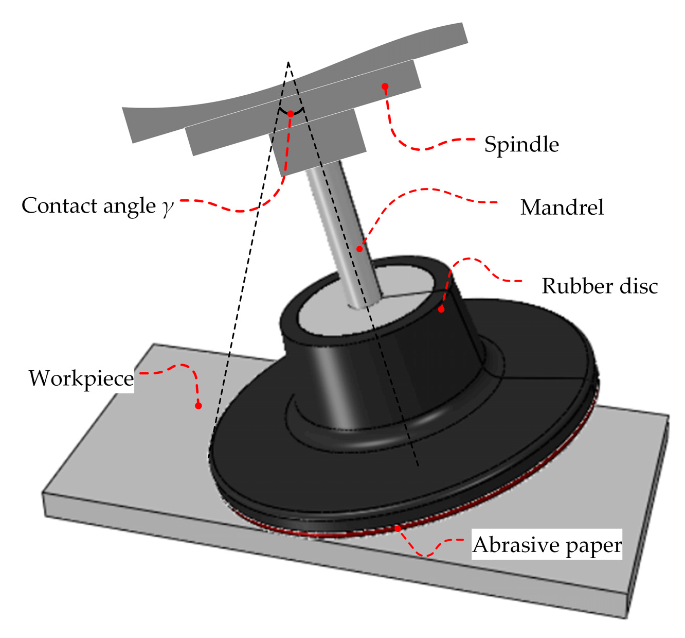
2. Characteristics of the Abrasive Disc Grinding Process

The basic principle of the flexible abrasive disc grinding process is illustrated in Figure 1. The mandrel connected to the spindle drives the high-speed rotation of the abrasive disc. The abrasive paper is bonded to the underside of the hyper-elastic rubber disc. The contact between the abrasive grains and workpiece surface is created by the function of the grinding force. Acting as micro cutting edges, the material removal process is achieved by the relative movement of the abrasive grains against the workpiece. In combination with the servo movement of the machine tool, the task of precision machining of the workpiece is completed.

Unlike traditional grinding, abrasive disc grinding is a form of elastic contact grinding. The flexible abrasive disc grinding tool consists of an elastic rubber disc and sandpaper, on which abrasive grains are regularly distributed. The abrasive tool produces an elastic deformation when in contact with the workpiece, which can be adapted to different shapes and different positions of the grinding area.

However, the hardness of the rubber disc has a direct effect on the grinding condition. The contact area during grinding increases and the roughness decreases as the hardness of the rubber disc decreases. Conversely, as the hardness of the rubber backing increases, the contact area during grinding decreases and the roughness increases [29].

Simultaneously, affected by the contact angle, γ, during the grinding process, the effective grinding contact area significantly increases, resulting in a significant improvement in the grinding material removal efficiency. In addition to the effects of sliding, ploughing, and cutting, the abrasive disc grinding grains through the extrusion effect can also make the surface of the workpiece produce plastic deformation, cold and hard layer changes, surface cracks, thermoplastic flow, and other comprehensive effects.

Moreover, the abrasive grains are usually attached to the abrasive substrate through advanced processes, such as electrostatic sand planting. The geometry of the abrasive grains is generally long and triangular, with a uniform size, distribution, and grain protrusion height [30]. The elastic contact will increase the number of abrasive grains involved in grinding per unit of time, reduce the grinding force borne by a single abrasive grain, and improve the grinding quality, while reducing the abrasive wear ratio of the abrasive disc. Therefore, abrasive disc grinding is a precision machining process with multiple functions, such as grinding, lapping, and polishing.

3. Characteristics of the Abrasive Disc Grinding Process

In the elastic contact grinding process, the material removal depth depends on the pressure applied to the flexible abrasive grinding tool. Its true value is less than the programmed grinding depth, a_p, and this significant difference means that the conventional rigid grinding force model is not applicable to flexible abrasive disc grinding. In order to reveal the material removal mechanism of the abrasive disc grinding process, this manuscript analyzes the macroscopic contact force between the abrasive tool and the workpiece, as well as the microscopic contact force between the abrasive grains and the workpiece.

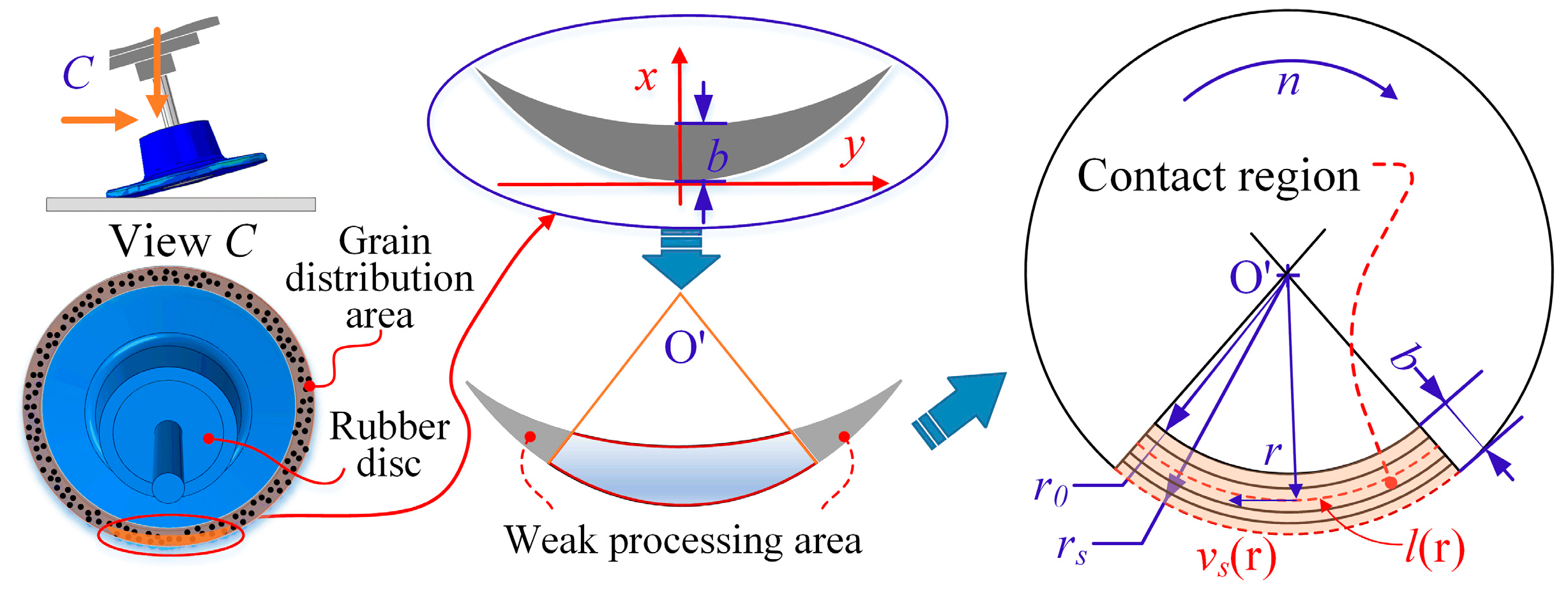
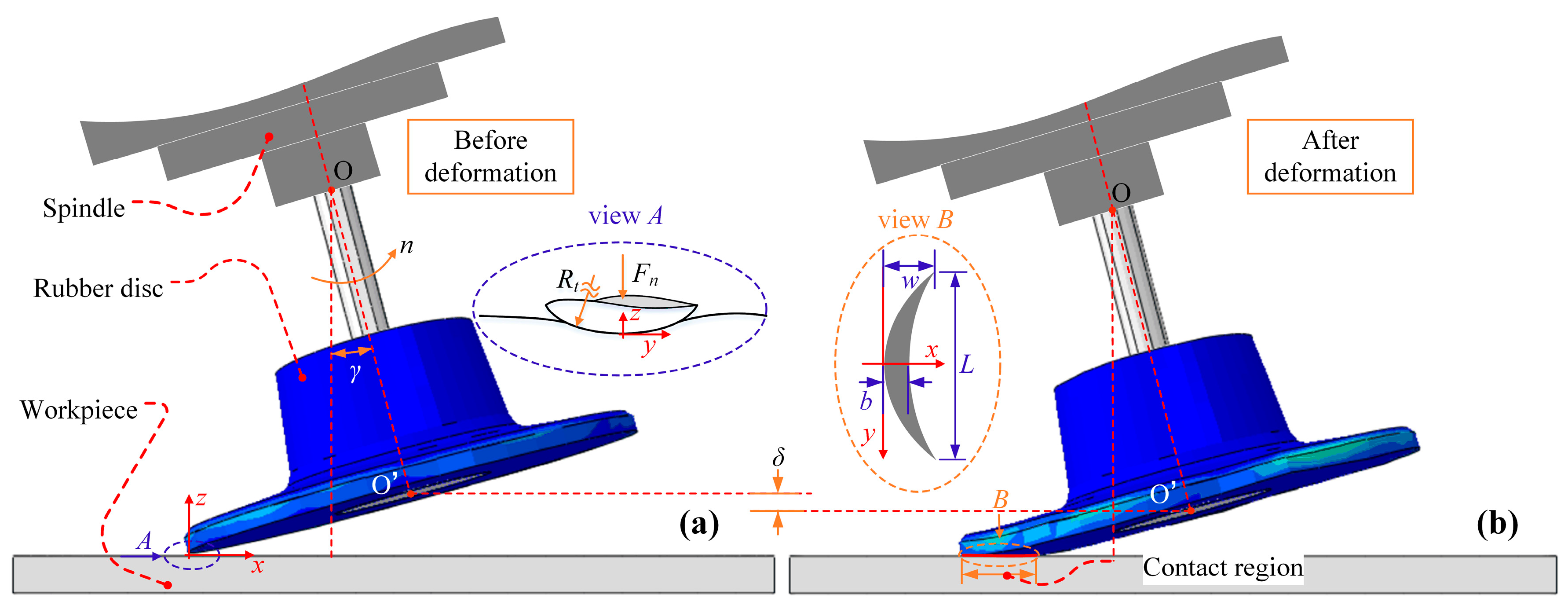
3.1. Macroscopic Grinding Force

Assuming the workpiece as a rigid body, the abrasive tool will cause elastic deformation while the abrasive tool is in contact with the surface of the workpiece, as shown in Figure 2. The three-dimensional profile is transformed into a one-dimensional profile using the method of dimensionality reduction (Figure 2a, view A). The deformation displacement under the contact pressure is denoted by δ, and the shape of the contact region is similar to that of the crescent (Figure 2b, view B). The normal contact force, F_n, can be regarded as the deformation force of the disc grinding tool. According to Hertz’s contact theory [31], it can be illustrated as:

$$F_n=\frac{4}{3}\cdot E^{*}\cdot R_t^{\raisebox{1ex}{$1$}\!\left/ \!\raisebox{-1ex}{$2$}\right.}\cdot {\delta }^{\raisebox{1ex}{$3$}\!\left/ \!\raisebox{-1ex}{$2$}\right.}$$

(1)

where E^* denotes the equivalent Young’s modulus of the disc grinding tool, R_t denotes the radius of curvature of the contact section between the rubber disc and the workpiece, and δ denotes the displacement of the rubber disc perpendicular to the surface of the workpiece after deformation.

The equivalent Young’s modulus, E^*, can be calculated by Equation (2) [31]:

$$E^{*}=\frac{1-v_1^2}{E_1}+\frac{1-v_2^2}{E_2}$$

(2)

where E₁ and v₁ are the Young’s modulus and Poisson ratios of the rubber disc, respectively, and E₂ and v₂ are the Young’s modulus and Poisson ratios of the sandpaper substrate.

The radius of curvature, R_t, can be expressed as:

$$R_t={\left({\left(1+\frac{d\mathrm{z}}{dy}\right)}^2\right)}^{\raisebox{1ex}{$3$}\!\left/ \!\raisebox{-1ex}{$2$}\right.}/\left|\frac{d^{2}z}{d^{2}y}\right|$$

(3)

where dz/dy represents the slope of the curve at this point, and d²z/d²y represents the second derivative of the curve at this point.

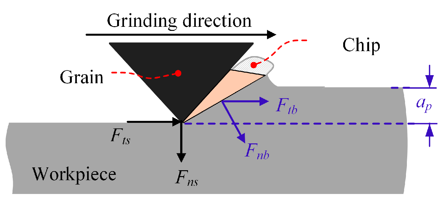
3.2. Microscopic Grinding Force

The mathematical model of grinding force established by scholars has taken into account the stochastic characteristics of the distribution of the grinding edge around the grinding wheel and the dynamic situation of the grinding process [32]. However, with the gradual increase of the top dulling plane of the abrasive grain, the grinding force is also gradually increased, so the above mathematical model of the grinding force cannot be illustrated intuitively. Therefore, the microscopic grinding force of a single abrasive grain is divided into two parts: chip deformation force and friction force. Assuming that the abrasive grains are conical, the force process between the abrasive grain and the workpiece is shown in Figure 3. Both normal and tangential grinding forces have two components, as shown in Equation (4) [33]:

$$\left\{\begin{array}{c}{F}_{ng}=F_{nc}+F_{ns}\\ F_{tg}=F_{tc}+F_{ts}\end{array}\right.$$

(4)

where F_ng and F_tg represent the normal contact force and tangential contact force of single grain, respectively, F_nc and F_tc represent the normal grinding force and tangential grinding force due to chip deformation, respectively, and F_ns and F_ts represent the normal grinding force and tangential grinding force due to friction, respectively.

This manuscript focuses on the study of normal grinding force, F_n, as it is the basis of the material removal effects according to the Preston Equation. For a single abrasive grain, the normal grinding force due to chip deformation and friction can be illustrated by Equation (5) [33]:

$$\left\{\begin{array}{c}{F}_{nc}=K\cdot Q\\ F_{ns}=\overline{s}\cdot \overline{p}\end{array}\right.$$

(5)

where K denotes the grinding force per unit grinding area, N/mm², Q denotes the grinding cross-sectional area, mm², $\overline{s}$ denotes the average dull surface area of a single grain, i.e., the actual contact area between the working grain and the workpiece, mm², and $\overline{p}$ denotes the average contact pressure between the abrasive grain and the workpiece, which is proportional to the hardness of the material, N/mm². Combining Equations (4)–(6), the normal grinding force of a single grain, F_ng, can be expressed as:

$$F_{ng}=K\cdot Q+\overline{s}\cdot \overline{p}$$

(6)

The normal grinding force per unit grinding width, F_n′, acting between the abrasive tool and the workpiece, is equal to the sum of the normal forces of all the working abrasive grains in the contact area. It can be expressed as [34]:

$$F_n^{\prime }={\displaystyle \sum F_{ng}}={\displaystyle \sum F_{nc}}+{\displaystyle \sum F_{ns}}=K{\displaystyle \sum Q+N_d}\overline{s}\overline{p}$$

(7)

where N_d denotes the number of working grains per unit grinding width, and ∑Q denotes the sum of the cutting cross-sectional area of the abrasive grains per unit grinding width, respectively. N_d and ∑Q can be calculated as follows [34]:

$$\left\{\begin{array}{c}{\displaystyle \sum Q=\frac{v_w}{v_s}}\cdot a_p\\ N_d={\displaystyle {\int }_0^{l_s}{N}_d(l)dl}=\frac{A_n}{1+\alpha }{C}_e^{\beta }{\left(v_w/v_s\right)}^{\alpha }{a}_p^{(1+\alpha )/2}{d}_{se}^{(1-\alpha )/2}\end{array}\right.$$

(8)

where v_w denotes the linear velocity of the abrasive grains in the contact length, l, v_s denotes the workpiece velocity, l_s denotes the actual contact length, A_n denotes the coefficient related to the number of dynamic cutting edges, α, β, and C_e denote the coefficients related to the cutting edge shape and its distribution, and d_se denotes the diameter of the grinding edge. The normal grinding force, F_n′, can, therefore, be expressed as [34]:

$${F_n}^{\prime }=K\frac{v_w}{v_s}{a}_p+\frac{A_n}{1+\alpha }{C}_e^{\beta }{\left(v_w/v_s\right)}^{\alpha }{a}_p^{(1+\alpha )/2}{d}_{se}^{(1-\alpha )/2}\overline{s}\overline{p}$$

(9)

In the abrasive disc grinding process, the real contact region is as shown in Figure 2b, view B. Since the grinding material removal is concentrated in the center of the crescent region, the contact region can be simplified, as shown in Figure 4. The linear velocity, v_s(r), of the abrasive grain on any contact arc in the grinding region and the diameter of the grinding edge, d_se, can be expressed as a function of the curve radius, as shown in Equation (10):

$$\left\{\begin{array}{c}{v}_s=2\pi nr\\ d_{se}=2r\end{array}\right.$$

(10)

Combining the above equations, the normal grinding force per unit contact width is calculated by:

$$\left\{\begin{array}{l}{F}_n^{\prime }=A_1{r}^{-1}+A_2{r}^{\raisebox{1ex}{$1-3\alpha $}\!\left/ \!\raisebox{-1ex}{$2$}\right.}\\ A_1=\frac{K{v}_w{a}_p}{2\pi n},A_2=\frac{2^{\raisebox{1ex}{$1-\alpha $}\!\left/ \!\raisebox{-1ex}{$2$}\right.}{A}_n{C}_e^{\beta }{v}_w^{\alpha }{a}_p^{(1+\alpha )/2}\overline{s}\overline{p}}{\left(1+\alpha \right){\left(2\pi n\right)}^{\alpha }}\end{array}\right.$$

(11)

Therefore, the total normal grinding force, F_n, in the contact region can be viewed as the sum of F_n′ from r₀ to r_s, as shown in Equation (12):

$$\begin{array}{l}{F}_n={\displaystyle {\int }_{r_0}^{r_s}\left(A_1{r}^{-1}+A_2{r}^{\raisebox{1ex}{$1-3\alpha $}\!\left/ \!\raisebox{-1ex}{$2$}\right.}\right)}dr\\ \hspace{0.33em}\hspace{0.33em}\hspace{0.33em}=A_1(\ln r_s-\ln r_0)+\frac{2A_2}{3(1-\alpha )}(r_s^{\frac{3(1-\alpha )}{2}}-r_0^{\frac{3(1-\alpha )}{2}})\end{array}$$

(12)

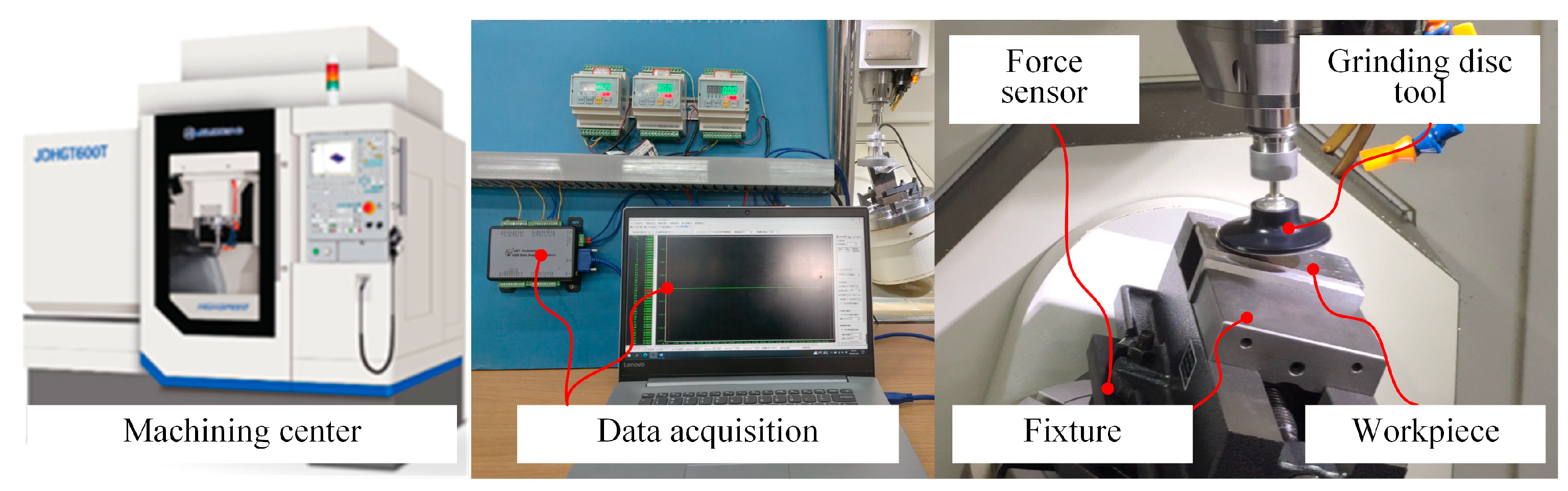
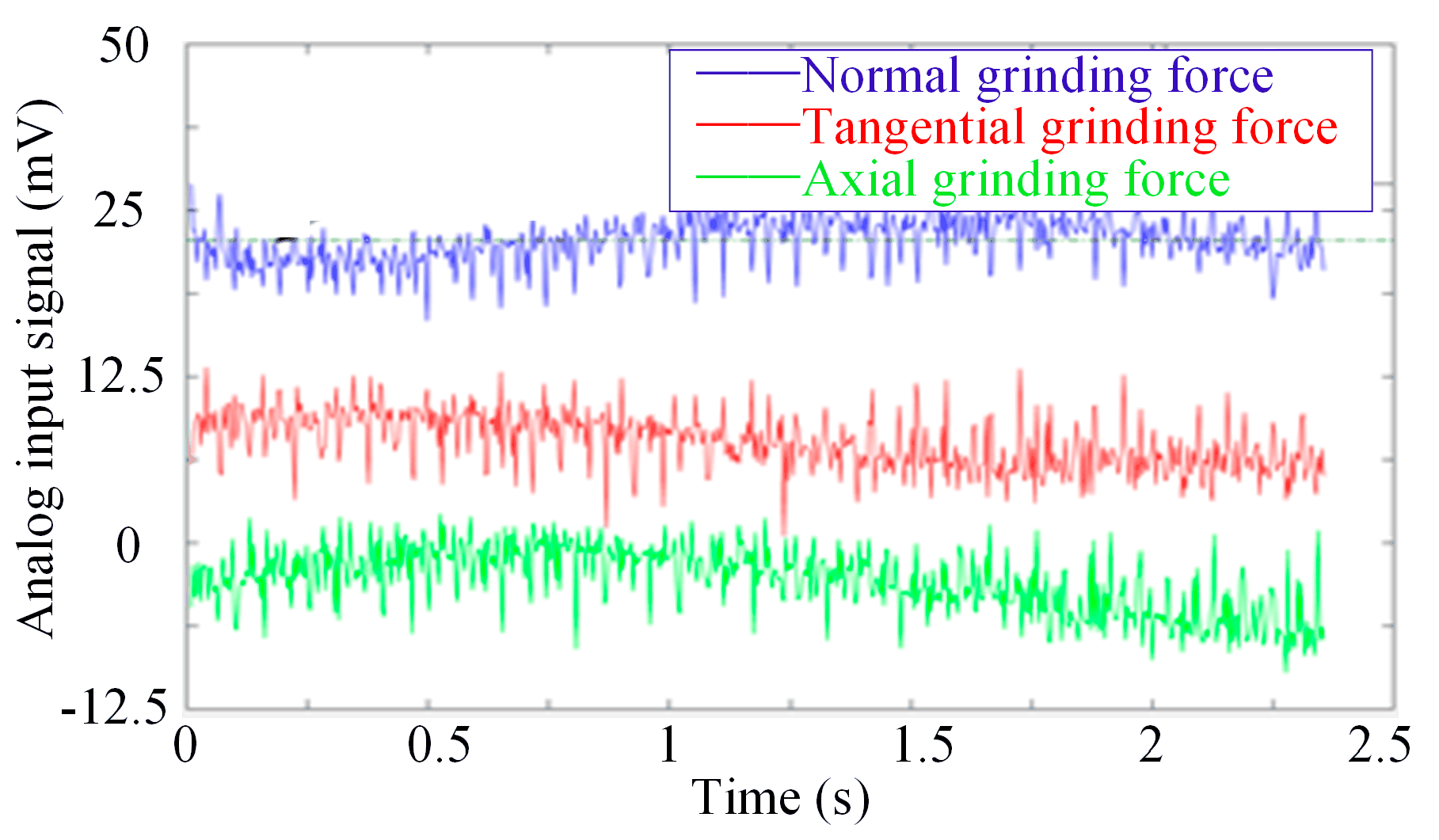
4. TC17 Abrasive Disc Grinding Experiment

In order to investigate the influencing factors of the grinding force of TC17 thin-walled components and their significance, a series of grinding experiments were carried out. A JDGR200 5-axis machining center from Beijing Jingdiao Group and LH-SZ-05 3-axis precision force sensor with a sensitivity of 1.0 ± 0.2 mV/V from Shanghai Liheng Sensor Technology Co. were selected. The grinding tool consisted of a 70 mm-diameter rubber disc and a 150# grain size silicon carbide abrasive paper. Thin-walled TC17 components with dimensions of 100 mm × 50 mm × 5 mm were selected as the workpiece to be machined. The experimental setup was constructed as shown in Figure 5.

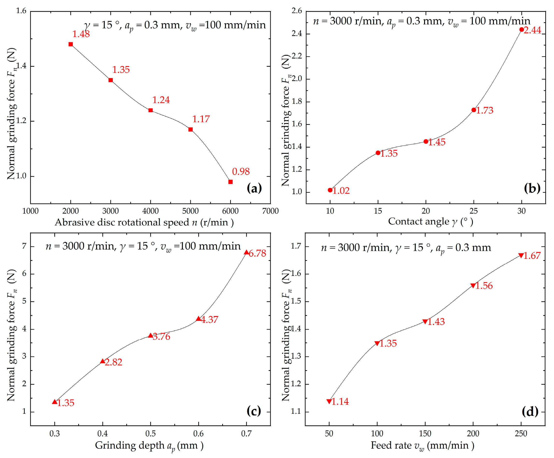
4.1. Influence of Grinding Parameters on Normal Force

The abrasive disc rotational speed, n (r/min), the contact angle, γ (°), the grinding depth, a_p (mm), and the workpiece feed rate, v_w (mm/min), were the main process parameters of the abrasive disc grinding. In order to investigate the influence of individual factors on the normal grinding force of the TC17 thin-walled workpiece, 16 sets of single-factor experiments were designed, and the experimental conditions are shown in

Table 1. Experimental conditions.

	Parameter	n (r/min)	γ (°)	ap (mm)	vw (mm/min)
No.
1		2000, 3000, 4000, 5000, 6000	15	0.3	100
2		3000	10, 15, 20, 25, 30	0.3	100
3		3000	15	0.3, 0.4, 0.5, 0.6, 0.7	100
4		3000	15	0.3	50, 100, 150, 200, 250

.

During the grinding experiments of the TC17 thin-walled workpiece, the LH-SZ-05 force sensor was used to monitor and collect the grinding force signal in real time, as shown in Figure 6, and the collected force signal was converted into a voltage signal and transferred to the USB3104A data acquisition card. Then, the sampled data were processed by MATLAB R2018b software, and the average value was obtained to represent the grinding force. The normal grinding forces obtained under different grinding conditions are shown in Figure 7.

As shown in Figure 7a, the experimental results showed that the normal grinding force decreased from 1.48 to 0.98 N, as the abrasive disc rotational speed increased from 2000 r/min to 6000 r/min. The main reason for this is that as the disc rotational speed increased, the time that the abrasive grains were involved in grinding the workpiece significantly decreased. As a result, the grinding effect of a single abrasive grain was weakened, and the actual material removal depth was reduced, which ultimately resulted in a reduction of the normal grinding force in the grinding area.

From the experimental results shown in Figure 7b, it can be seen that the normal grinding force increased from 1.02 N to 2.44 N, as the contact angle, γ, increased from 10° to 30°. As the contact angle increased, the grinding force gradually increased. The overall trend showed an initial slow increase, followed by an accelerated increase. The main reason for this is that the blunting effect of the abrasive grain on the cutting edge was enhanced as the contact angle increased. The negative front angle of the abrasive grains involved in the process increased, causing the friction between the abrasive tool and the workpiece to significantly increase. The final result was a reduction in the grinding contact area and an increase in the normal grinding force.

The grinding results showed that the effect of the grinding depth on the normal grinding force was very significant, as shown in Figure 7c. As the grinding depth increased from 0.3 mm to 0.7 mm, the normal grinding force increased from 1.35 N to 6.78 N, which was more than four times greater. This is because as the grinding depth increased, the actual depth of the abrasive grain cutting into the surface of the workpiece increased, while the number of abrasive grains involved in the grinding process increased. As a result, the volume of material removed by grinding significantly increased and the maximum undeformed chip thickness increased. Ultimately, the rate of change of the normal grinding force dramatically increased.

The normal grinding force results in Figure 7d show that as the feed rate, v_w, increased from 50 mm/min to 250 mm/min, the normal grinding force increased from 1.14 N to 1.67 N. It can be seen that the grinding force increased slightly with the increase of the feed rate. As the feed rate increased, the cutting thickness of each abrasive grain increased, and the contact length between the grinding tool and the workpiece increased. Simultaneously, the number of abrasive grains participating in the grinding increased, and the amount of material removed by grinding per unit time increased. This ultimately increased the normal grinding force. However, as the feed rate increased, the contact time between the abrasive grains and the workpiece decreased, resulting in a relatively minor impact.

4.2. Multi-Factor Orthogonal Experiment

In order to investigate the interactive effect of multiple factors on the normal grinding force, a four-factor, three-level orthogonal experimental scheme was designed in this manuscript using the Box–Behnken design (BBD) module. Feed rate, v_w, contact angle, γ, rotational speed, n, and grinding depth, a_p, were identified as A, B, C, and D, respectively, and used to investigate their effects on the normal grinding force. Three levels were set for each factor, −1, 0, and 1. According to the experimental results of the influence of each single factor on the grinding force, the values of the process parameters corresponding to different levels of each factor are shown in

Table 2. Levels of grinding process factors.

Level of Factor	A	B	C	D
	Feed Rate, vw/mm/min	Contact Angle, γ/°	Rotational Speed, n/r·min−1	Grinding Depth, ap/mm
−1	50	10	2000	0.3
0	100	20	3000	0.4
1	150	30	4000	0.5

.

The experimental design was carried out according to the response surface method, and a total of 29 sets of grinding process parameters were carried out to measure the normal grinding force at different factor levels. The obtained results were averaged as the responses, which are shown in

Table 3. Experimental scheme and results of BBD.

No.	Factors				Response		Factors				Response
	vw (mm/min)	γ (°)	n (r/min)	ap (mm)	Fn (N)	No.	vw (mm/min)	γ (°)	n (r/min)	ap (mm)	Fn (N)
1	100	20	3000	0.4	3.329	16	100	20	4000	0.3	1.306
2	100	30	3000	0.3	2.440	17	150	30	3000	0.4	4.420
3	50	10	3000	0.4	2.143	18	50	20	3000	0.3	1.596
4	100	20	2000	0.3	1.691	19	50	30	3000	0.4	4.299
5	50	20	4000	0.4	3.498	20	100	20	3000	0.4	3.153
6	50	20	3000	0.5	3.701	21	100	10	3000	0.5	3.697
7	100	20	2000	0.5	4.320	22	150	20	3000	0.5	5.086
8	100	20	3000	0.4	3.214	23	150	20	4000	0.4	3.657
9	150	20	3000	0.3	1.741	24	100	20	4000	0.5	4.325
10	150	20	2000	0.4	3.560	25	100	10	3000	0.3	1.020
11	100	30	4000	0.4	3.791	26	100	20	3000	0.4	3.505
12	50	20	2000	0.4	3.699	27	100	10	4000	0.4	2.214
13	150	10	3000	0.4	2.249	28	100	30	2000	0.4	4.063
14	100	20	3000	0.4	3.034	29	100	10	2000	0.4	2.708
15	100	30	3000	0.5	5.204

.

5. Prediction Model of Normal Grinding Force

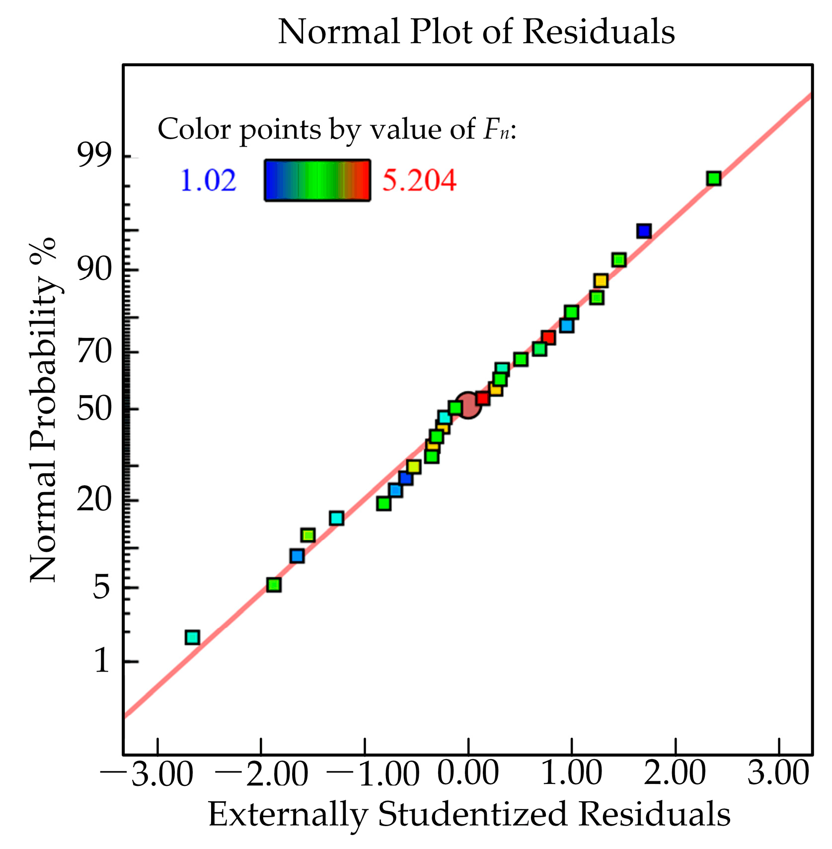
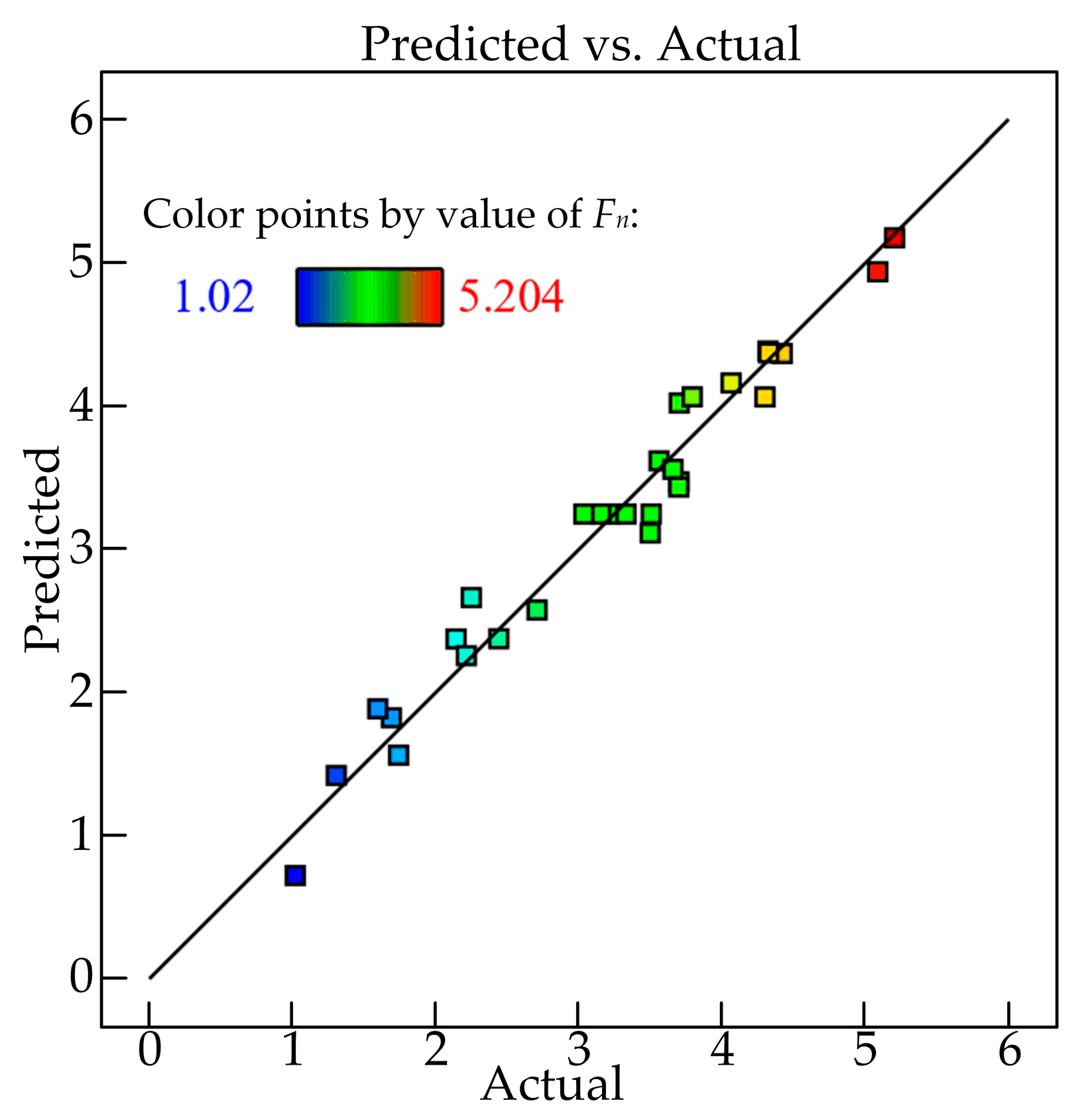
5.1. Analysis of the Experimental Results Using Response Surface Optimization

The polynomial regression model equation of normal grinding force, F_n, versus feed rate A, contact angle B, rotational speed C, and grinding depth D, was obtained in Design-Expert software (version numaber v13.0.1.0) as:

$$\begin{array}{l}{F}_n=3.25+0.1481A+0.8488B-0.1042C+1.38D\\ \hspace{0.33em}\hspace{0.33em}\hspace{0.33em}+0.0038AB+0.0745AC+0.3100AD+0.0555BC+0.0217BD\\ \hspace{0.33em}\hspace{0.33em}\hspace{0.33em}+0.0975CD+0.1481A^2-0.0270B^2+0.0460C^2-0.2921D^2\end{array}$$

(13)

In order to assess the degree of fit of the regression equation to the model, an ANOVA was carried out, and the results are presented in

Table 4. Variance analysis of the normal grinding force.

Source	Sum of Squares	df	Mean Square	F Value	p-Value
Model	33.16	14	2.37	28.37	<0.0001
A	0.2631	1	0.2631	3.15	0.0976
B	8.65	1	8.65	103.55	<0.0001
C	0.1302	1	0.1302	1.59	0.2322
D	22.79	1	22.79	272.99	<0.0001
AB	0.0001	1	0.0001	0.0007	0.9797
AC	0.0222	1	0.0222	0.2659	0.6142
AD	0.3844	1	0.3844	4.60	0.0499
BC	0.0123	1	0.0123	0.1476	0.7067
BD	0.0019	1	0.0019	0.0227	0.8825
CD	0.0380	1	0.0380	0.4554	0.5108
A2	0.1423	1	0.1423	1.70	0.2128
B2	0.0047	1	0.0047	0.0566	0.8154
C2	0.0137	1	0.0137	0.1644	0.6913
D2	0.5535	1	0.5535	6.63	0.0220
Residual	1.17	14	0.0835
Lack of fit	1.04	10	0.1040	3.24	0.1345
Pure error	0.1286	4	0.0321
Cor total	34.33	28

. The F value reflects the extent to which the model component contributes to the effect of the response value, with a larger F value indicating a greater effect of the factor. The regression model was statistically significant at p < 0.01 for highly significant differences and p < 0.05 for significant differences, indicating that the test model was statistically significant. Table 4 shows that the F value of the model was 28.37, with p < 0.0001, indicating that the regression equation was highly significant and reliable. The F value of the lack-of-fit term was 3.24, with p = 0.1345 > 0.05, indicating a small error and a better fit for the regression equation. Therefore, the established model can be used to analyze and predict the test results. B, D, AD, and D2 were the more influential factors, with B and D having a highly significant effect on the normal grinding force. Depending on the magnitude of F, the factors affecting the normal grinding force were, in order of magnitude, the grinding depth, contact angle, feed rate, and rotational speed.

The model fit statistics are shown in

Table 5. Fitting statistical information.

Name	Value	Name	Value
Std.Dev.	0.2890	R2	0.9659
Mean	3.20	Adjusted R2	0.9319
C.V.%	9.04	Predicted R2	0.8196
		Adeq Precision	21.4325

. As can be seen from the table, the model had a decision coefficient, R², of 0.9659, which is close to 1, indicating that the model explained 96.59% of the experimental data. The adjusted R² = 0.9319 and predicted R² = 0.8196, and their difference was 0.1123, which is less than 0.2. This indicates that the fit of the model is reliable, and it can be effectively used to the predict the normal grinding force. The depth accuracy (signal-to-noise ratio) of the model was 21.4325, which is greater than 4 [35], further indicating that the model has high accuracy.

The normal distribution of the normal grinding force residuals is shown in Figure 8. The residuals of each response target in the figure were approximately linearly distributed with no serious deviation from the trajectory, indicating that the residual distribution was random. Therefore, the model fit the random error well, extracted all the predictable parts, and was well adapted to the needs of response target prediction. The comparison between the tested and the predicted values of the normal grinding force is shown in Figure 9. It can be seen that the distribution of points on the graph was close to a straight line, indicating that the results obtained by the model are in good agreement with the experimental results and are consistent.

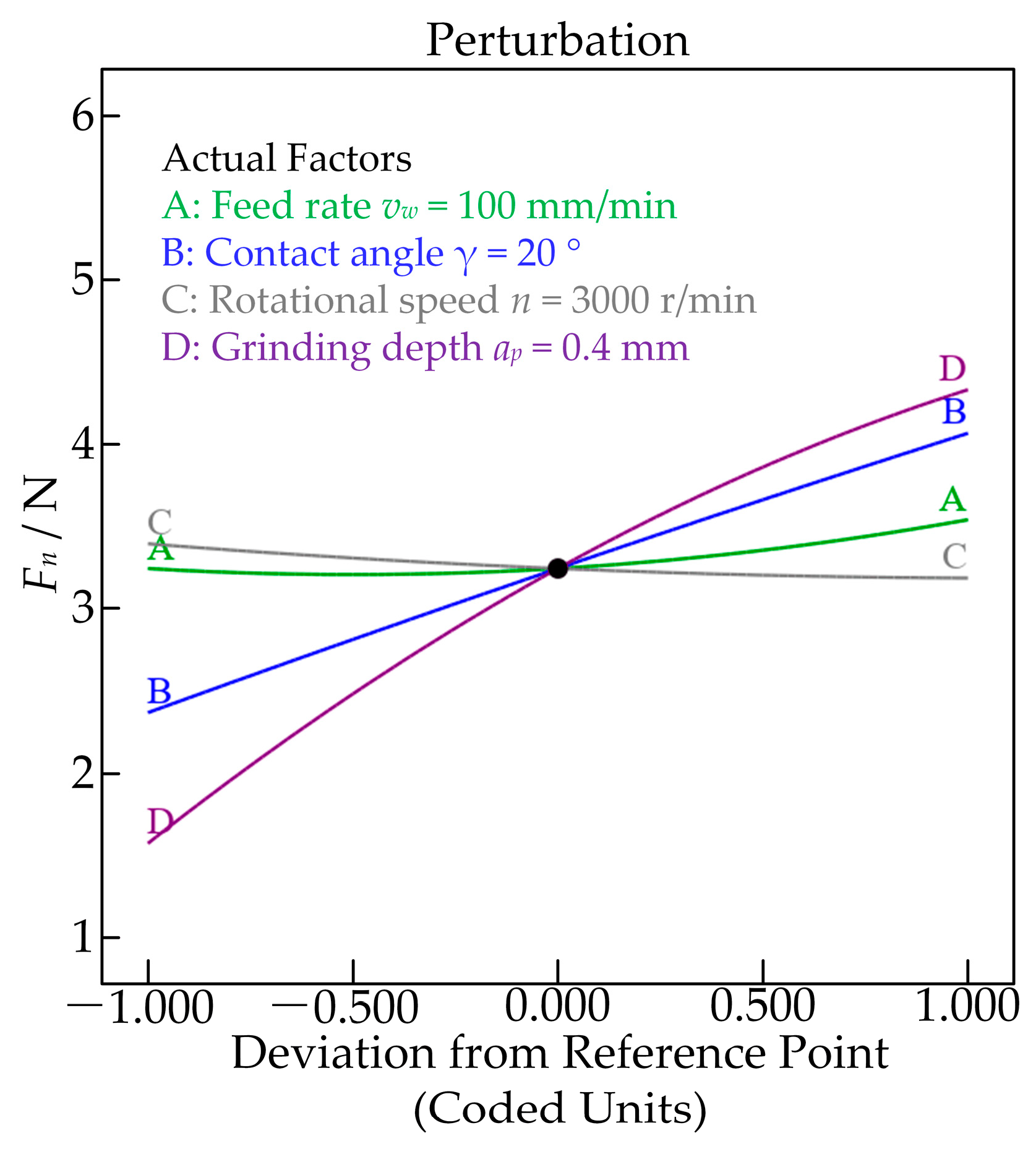
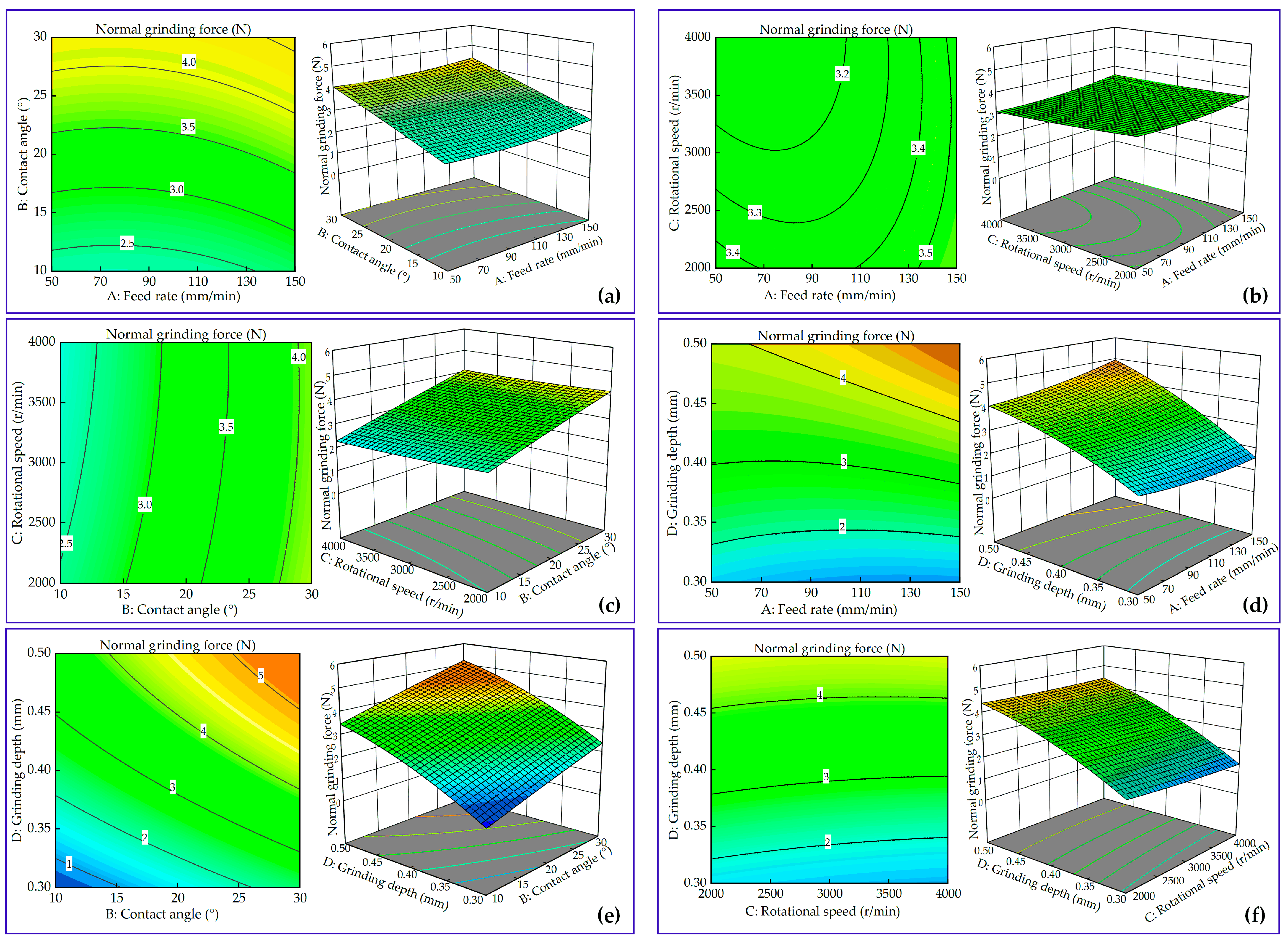
5.2. Interaction Effect of Process Parameters on Normal Grinding Forces

The residual normal distribution plot proves the reliability of the model, while the perturbation plot (Figure 10) can visualize the influence of each process parameter on the normal grinding force. With the gradual increase of B (contact angle) and D (grinding depth), the normal grinding force also increased. With the increase of C (abrasive disc rotational speed), the normal grinding force slightly decreased. With the increase of A (feed rate), the normal grinding force did not change significantly. From the figure, it can be seen that B (contact angle) and D (grinding depth) had a greater effect on the normal grinding force, while A (feed rate) and C (abrasive disc rotational speed) had a smaller effect on it.

Contours and response surfaces provide a direct and accurate representation of the interaction between two factors, showing the effects of different factors on an indicator. Figure 11a–f show the effects of the interaction of the other two factors on the response value when each factor was at the center value. The figures illustrate that the interaction of A and D had the largest effect, while the interaction of B and D had the smallest effect. When A was fixed, F_n significantly decreased as D decreased, and when D was fixed, F_n tended to increase as A increased.

5.3. Prediction of Normal Grinding Force Based on PSO-BP

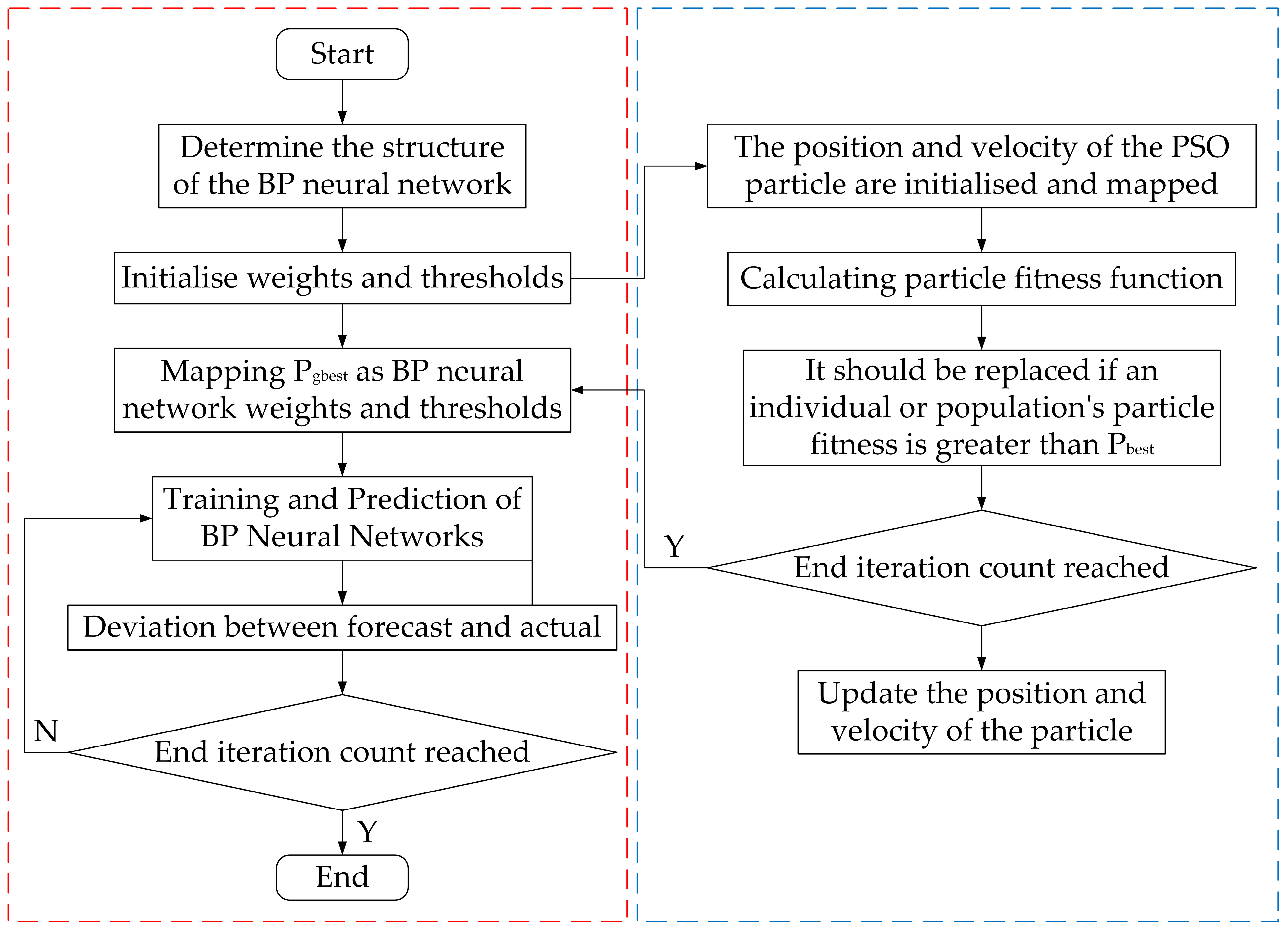
5.3.1. Principle of PSO-BP Neural Network

The BP (backpropagation) algorithm is a commonly used neural network training algorithm that adjusts the weights and biases of the neural network by backpropagating errors. The BP algorithm updates the weights and biases of the network based on the error by calculating the error between the actual output and the desired output and propagating the error back through the different levels of the network.

The PSO (particle swarm optimization) algorithm is an optimization algorithm based on group intelligence, which simulates the behavior of biological groups, such as birds or fish. In the PSO algorithm, each individual is known as a particle, and each particle has a position and velocity that is updated based on its own experience and the experience of the group to find the optimal solution.

The PSO-BP algorithm is an optimization algorithm that combines the PSO algorithm and the BP algorithm. The PSO-BP algorithm is mainly used to train neural networks. By optimizing the weights and biases of the neural network, it enables the neural network to better fit the training data. Its advantage is that it can avoid the problem that the BP algorithm easily falls into the local optimal solution, and it can better search the parameter space of the neural network by introducing the global search capability of the PSO algorithm. At the same time, the PSO-BP algorithm can also accelerate the training speed of the neural network and improve the training efficiency. Its operation principle is shown in Figure 12.

5.3.2. Analysis of PSO-BP Neural Network Prediction Results

The data in Table 3 were imported into the MATLAB Neural Network Toolbox, and 29 sets of orthogonal experiments were divided into 2 classes, where the training set (training data) accounted for about 70% (20 sets) of the total data and the testing set (testing data) accounted for about 30% (9 sets) of the total data. The Levenberg–Marquardt algorithm was selected to train the neural network, and the training results are shown in Figure 13. The training results of the neural network converged at six steps, and the error was less than 1 × 10⁻⁶, which meets the requirements of prediction accuracy.

To verify the accuracy and reliability of the prediction model, a comparison between the predicted value and the actual value of the PSO-BP neural network is shown in Figure 14. The results showed that the predicted values were quite close to the actual values, with errors mostly within 0.5. Using formulas to calculate the relevant index parameters of the prediction model, it can be obtained that the determination coefficients, R², of the training and test set data were 0.93135 and 0.93678, respectively. The MAE (mean absolute error) of the training and the test set data was 0.14442 and 0.22938, respectively, and the MRE (mean relative error) of the training and the test set data was 4.2% and 0.7%, respectively. Compared with the prediction model of the response surface method, the coefficient of determination, R², of the BBD model was 0.9686, which is larger than the absolute coefficient of the PSO-BP neural network. This indicates that the BBD model is more accurate. Therefore, the selection of the response surface prediction model has more guiding significance for controlling the normal grinding force and adjusting the surface accuracy of TC17.

5.4. Comparison of the Results of Two Prediction Models

The generalization ability of a learning method refers to the predictive ability of the model learned by the method on unknown data. It is an essential property of learning methods and, in practice, the generalization ability of learning methods is usually evaluated by testing errors. Eight groups of data from the single-factor experiments (as shown in

Table 6. Comparison of the prediction results of the two models with new datasets.

Sample	vw (mm/min)	α (°)	n (r/min)	ap (mm)	Experiment Value (N)	BBD Predicted Value (N)	PSO-BP Predicted Value (N)
1	100	15	3000	0.4	2.82	2.814	2.755
2	100	15	3000	0.5	3.76	3.889	3.948
3	100	15	2000	0.3	1.48	1.430	1.315
4	100	15	4000	0.3	1.24	0.971	1.061
5	50	15	3000	0.3	1.14	1.468	1.041
6	250	15	3000	0.3	1.67	1.983	1.104
7	100	20	3000	0.3	1.45	1.575	1.752
8	100	30	3000	0.3	2.44	2.375	2.695

) were selected as prediction samples to verify the generalization ability of the two prediction models. The BBD and PSO-BP prediction models were fitted, and the comparison between the predicted values and the experimental values is shown in Figure 15.

The analysis showed that the maximum absolute error, the minimum absolute error, and the MAE between the BBD prediction results and the experimental values were about 0.328 N, 0.006 N, and 0.161 N, respectively. In the prediction results of the PSO-BP model, these three errors were 0.566 N, 0.065 N, and 0.227 N, respectively. In addition, the maximum relative error, the minimum relative error, and the mean relative error of the BBD prediction results were about 28.772%, 0.213%, and 10.939%, respectively, and these were about 33.982%, 2.305%, and 13.343%, respectively, in the prediction results of the PSO-BP model. The comparison results showed that the BBD model had a slightly smaller MAE and MRE than the PSO-BP model, and the range of variation was also smaller. Therefore, the BBD response surface method is more accurate as a normal contact force prediction algorithm.

Consequently, in the abrasive disc grinding process for TC17, the prediction model of the normal grinding force with high reliability based on the BBD response surface method was developed from the experimental data in this study. Additionally, the effects of workpiece curvature and random distribution of abrasive grains on the grinding force and material removal mechanism will be considered in future work through both finite element simulation and experimental methods.

6. Conclusions

(1)

The abrasive disc grinding process was analyzed and considered as a flexible process to adapt to different curved surfaces. The normal grinding force model was established from macroscopic and microscopic perspectives, which showed that the contact angle, grinding depth, rotational speed, and feed rate were the main factors.

(2)

The normal grinding force significantly increased with the increase of the grinding depth and contact angle, slightly increased with the increase of the feed rate, and slightly decreased with the increase of the rotational speed. The regression model of normal grinding force was developed, and the ANOVA results showed that the interaction of the feed rate and grinding depth was the more influential factor.

(3)

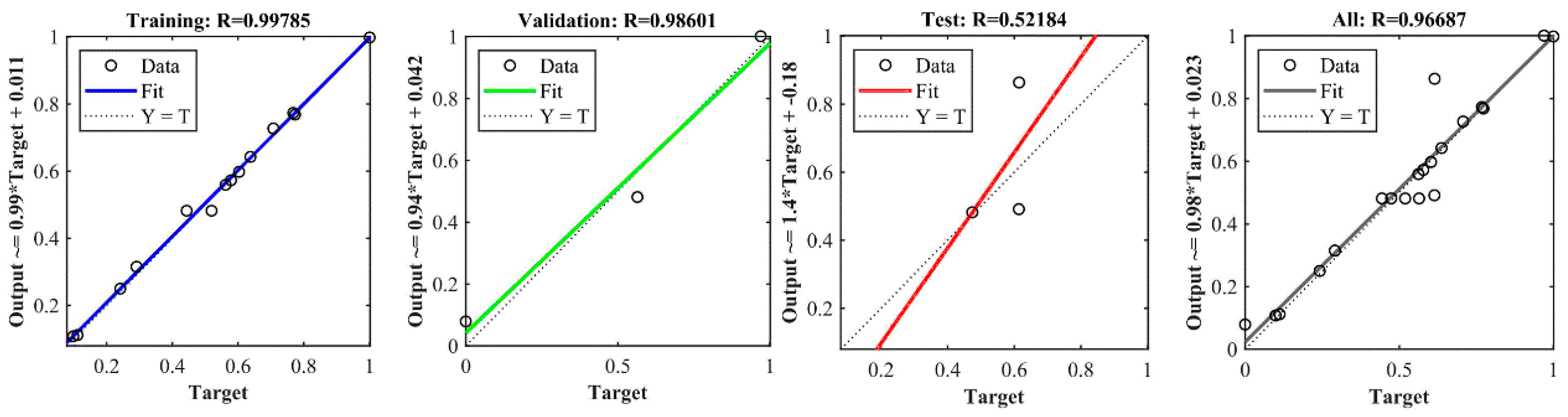
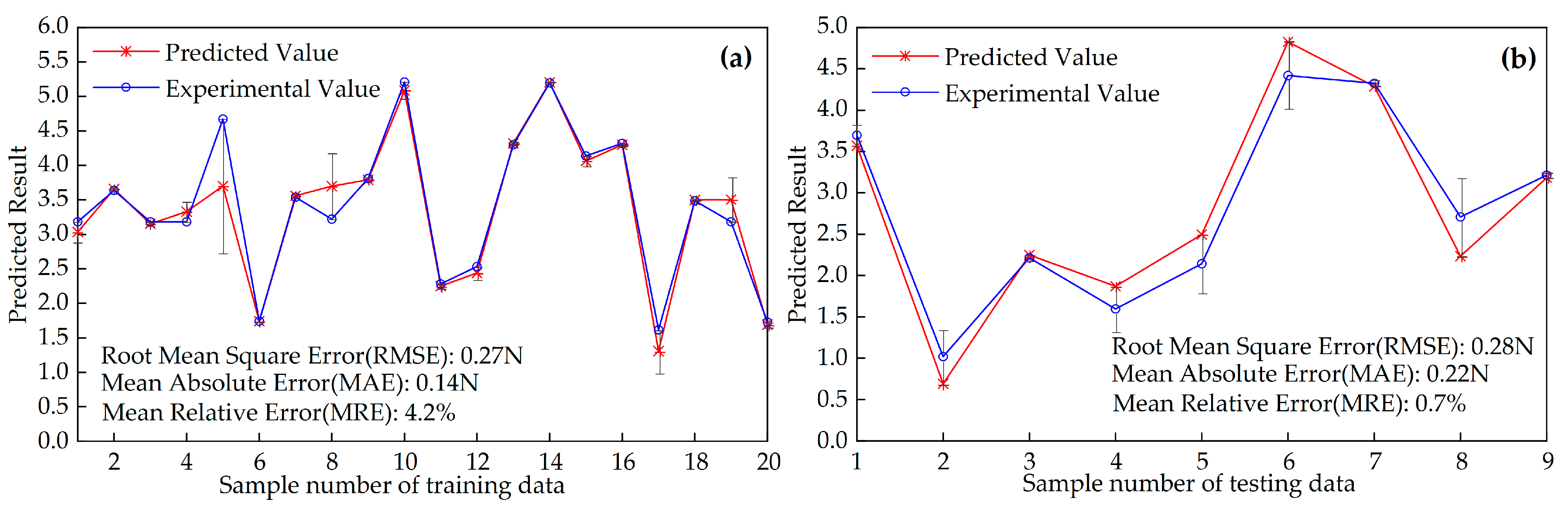
The normal grinding force prediction model based on the PSO-BP neural network was carried out. The coefficient of determination, R², of the training and test set data verified the accuracy and reliability of the model. The maximum absolute and relative errors of the training and test data in the model were 0.22 N and 4.2%, respectively.

(4)

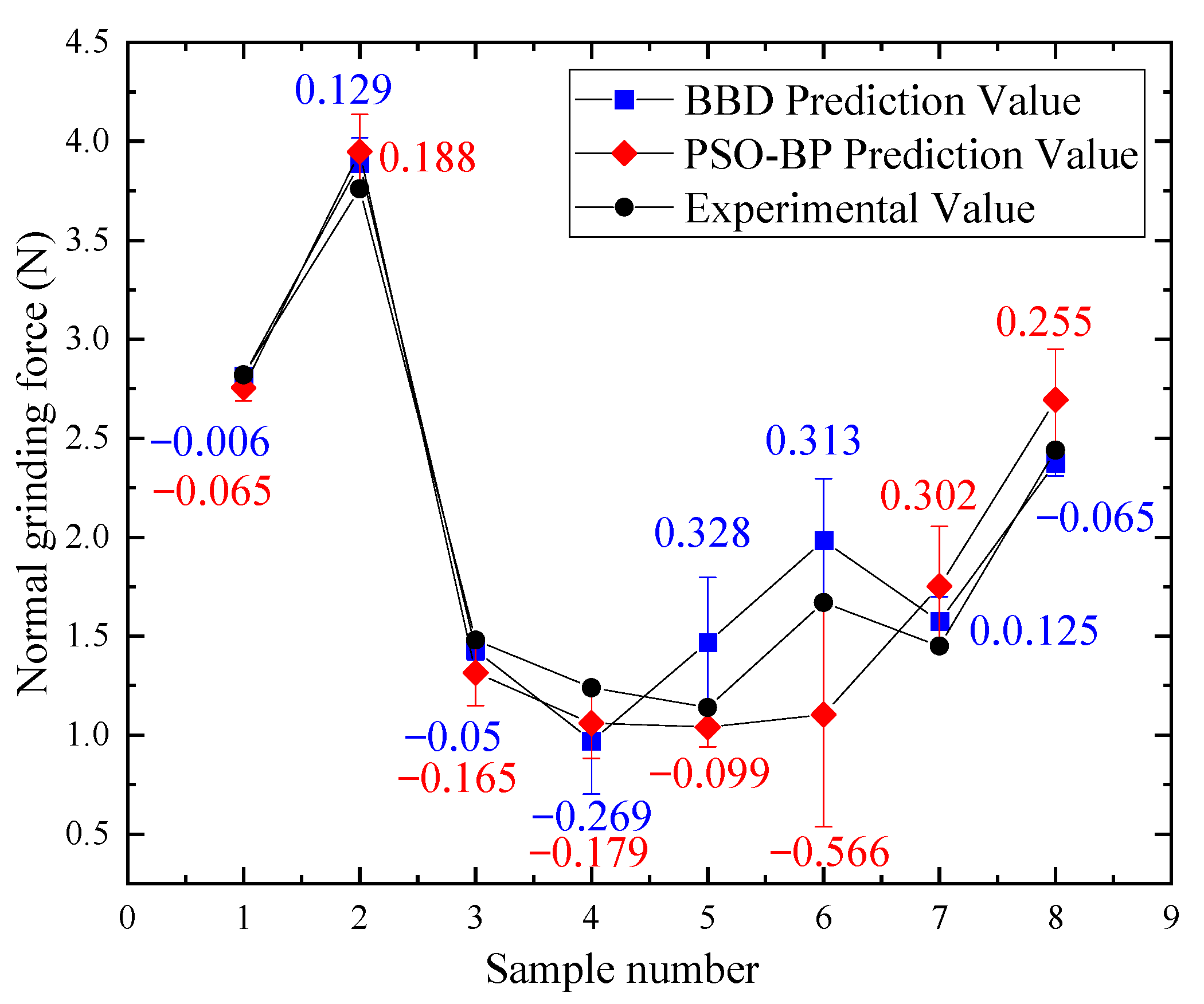
Comparing the PSO-BP and BBD prediction models and their generalization ability, the added prediction experimental results showed that the MAE and MRE of the above two prediction models were 0.22 N and 0.16 N, and 13.3% and 10.9%, respectively. The results showed that the BBD model was more effective and accurate in predicting the normal grinding force.

References

1. Zhao, Q.; Sun, Q.; Xin, S.; Chen, Y.; Wu, C.; Wang, H.; Xu, J.; Wan, M.; Zeng, W.; Zhao, Y. High-strength titanium alloys for aerospace engineering applications: A review on melting-forging process. Mater. Sci. Eng. A 2022, 845, 143260. [Google Scholar] [CrossRef]
2. Williams, J.C.; Boyer, R.R. Opportunities and Issues in the Application of Titanium Alloys for Aerospace Components. Metals 2020, 10, 705. [Google Scholar] [CrossRef]
3. Chen, L.-Y.; Cui, Y.-W.; Zhang, L.-C. Recent Development in Beta Titanium Alloys for Biomedical Applications. Metals 2020, 10, 1139. [Google Scholar] [CrossRef]
4. Arunachalam, A.P.S.; Idapalapati, S. Material removal analysis for compliant polishing tool using adaptive meshing technique and Archard wear model. Wear 2019, 418–419, 140–150. [Google Scholar] [CrossRef]
5. Arunachalam, A.P.S.; Idapalapati, S.; Subbiah, S.; Lim, Y.W. A novel retractable stiffener-based disk-shaped active compliant polishing tool. J. Manuf. Porcess. 2020, 51, 83–94. [Google Scholar] [CrossRef]
6. Yao, C.; Tan, L.; Yang, P.; Zhang, D. Effects of tool orientation and surface curvature on surface integrity in ball end milling of TC17. Int. J. Adv. Manuf. Technol. 2018, 94, 1699–1710. [Google Scholar] [CrossRef]
7. Chen, P.; Zhang, X.; Feng, M.; Li, S.; Pan, X.; Feng, W. Research on Adaptive Control of Grinding Force for Carbide Indexable Inserts Grinding Process Based on Spindle Motor Power. Machines 2022, 10, 802. [Google Scholar] [CrossRef]
8. Lei, X.; Xiang, D.; Peng, P.; Liu, G.; Li, B.; Zhao, B.; Gao, G. Establishment of dynamic grinding force model for ultrasonic-assisted single abrasive high-speed grinding. J. Mater. Process. Technol. 2022, 300, 117420. [Google Scholar] [CrossRef]
9. Bie, W.; Zhao, B.; Gao, G.; Chen, F.; Chen, H. Grinding force assessment in tangential ultrasonic vibration-assisted grinding gear: Analytical model and experimental verification. Int. J. Adv. Manuf. Technol. 2023, 126, 5457–5474. [Google Scholar] [CrossRef]
10. Li, H.; Chen, T.; Duan, Z.; Zhang, Y.; Li, H. A grinding force model in two-dimensional ultrasonic-assisted grinding of silicon carbide. J. Mater. Process. Technol. 2022, 304, 117568. [Google Scholar] [CrossRef]
11. Song, K.; Xiao, G.; Chen, S.; Liu, X.; Huang, Y. A new force-depth model for robotic abrasive belt grinding and confirmation by grinding of the Inconel 718 alloy. Robot. CIM-INT. Manuf. 2023, 80, 102483. [Google Scholar] [CrossRef]
12. Song, K.; Xiao, G.; Chen, S.; Li, S. Analysis of thermal-mechanical causes of abrasive belt grinding for titanium alloy. Int. J. Adv. Manuf. Technol. 2021, 113, 3241–3260. [Google Scholar] [CrossRef]
13. Li, L.; Ren, X.; Feng, H.; Chen, H.; Chen, X. A novel material removal rate model based on single grain force for robotic belt grinding. J. Manuf. Porcess. 2021, 68, 1–12. [Google Scholar] [CrossRef]
14. Yan, S.; Xu, X.; Yang, Z.; Zhu, D.; Ding, H. An improved robotic abrasive belt grinding force model considering the effects of cut-in and cut-off. J. Manuf. Porcess. 2019, 37, 496–508. [Google Scholar] [CrossRef]
15. Liu, M.; Li, C.; Zhang, Y.; Yang, M.; Gao, T.; Cui, X.; Wang, X.; Xu, W.; Zhou, Z.; Liu, B.; et al. Analysis of grinding mechanics and improved grinding force model based on randomized grain geometric characteristics. Chinese J. Aeronaut. 2023, 36, 160–193. [Google Scholar] [CrossRef]
16. Tao, H.; Liu, Y.; Zhao, D.; Lu, X. Prediction and measurement for grinding force in wafer self-rotational grinding. Int. J. Mech. Sci. 2023, 258, 108530. [Google Scholar] [CrossRef]
17. Yi, J.; Yi, T.; Deng, H.; Chen, B.; Zhou, W. Theoretical modeling and experimental study on grinding force of straight groove structured grinding wheel. Int. J. Adv. Manuf. Technol. 2023, 124, 3407–3421. [Google Scholar] [CrossRef]
18. Jamshidi, H.; Budak, E. An analytical grinding force model based on individual grit interaction. J. Mater. Process. Technol. 2020, 283, 116700. [Google Scholar] [CrossRef]
19. Jamshidi, H.; Gurtan, M.; Budak, E. Identification of active number of grits and its effects on mechanics and dynamics of abrasive processes. J. Mater. Process. Technol. 2019, 273, 116239. [Google Scholar] [CrossRef]
20. Jamshidi, H.; Budak, E. On the prediction of surface burn and its thickness in grinding processes. CIRP Ann. 2021, 70, 285–288. [Google Scholar] [CrossRef]
21. Ma, X.; Cai, Z.; Yao, B.; Chen, G.; Liu, W.; Qiu, K. Dynamic grinding force model for face gear based on the wheel-gear contact geometry. J. Mater. Process. Technol. 2022, 306, 117633. [Google Scholar] [CrossRef]
22. Cai, S.; Cai, Z.; Lin, C. Modeling of the generating face gear grinding force and the prediction of the tooth surface topography based on the abrasive differential element method. CIRP J. Manuf. Sci. Technol. 2023, 41, 80–93. [Google Scholar] [CrossRef]
23. Meng, Q.; Guo, B.; Wu, G.; Xiang, Y.; Guo, Z.; Jia, J.; Zhao, Q.; Li, K.; Zeng, Z. Dynamic force modeling and mechanics analysis of precision grinding with microstructured wheels. J. Mater. Process. Technol. 2023, 314, 117900. [Google Scholar] [CrossRef]
24. Ma, Z.; Wang, Q.; Chen, H.; Chen, L.; Qu, S.; Wang, Z.; Yu, T. A grinding force predictive model and experimental validation for the laser-assisted grinding (LAG) process of zirconia ceramic. J. Mater. Process. Technol. 2022, 302, 117492. [Google Scholar] [CrossRef]
25. Zhang, X.; Kang, Z.; Li, S.; Shi, Z.; Wen, D.; Jiang, J.; Zhang, Z. Grinding force modelling for ductile-brittle transition in laser macro-micro-structured grinding of zirconia ceramics. Ceram. Int. 2019, 45, 18487–18500. [Google Scholar] [CrossRef]
26. Zhang, X.; Jiang, J.; Li, S.; Wen, D. Laser textured Ti-6Al-4V surfaces and grinding performance evaluation using CBN grinding wheels. Opt. Laser. Technol. 2019, 109, 389–400. [Google Scholar] [CrossRef]
27. Zhou, H.; Ding, W.; Li, Z.; Su, H.-H. Predicting the grinding force of titanium matrix composites using the genetic algorithm optimizing back-propagation neural network model. P.I. Mech. Eng. B-J. Eng. 2019, 233, 1157–1167. [Google Scholar] [CrossRef]
28. Gu, P.; Zhu, C.; Tao, Z.; Yu, Y. A grinding force prediction model for SiCp/Al composite based on single-abrasive-grain grinding. Int. J. Adv. Manuf. Technol. 2020, 109, 1563–1581. [Google Scholar] [CrossRef]
29. Duan, J.; An, J.; Wu, Z.; Huai, W.; Gao, F. Contact characteristics and material removal mechanism of aerospace blade abrasive disc grinding. J. Mech. Eng. 2023, 59, 349–360. Available online: http://www.cjmenet.com.cn/CN/10.3901/JME.2023.17.349 (accessed on 7 February 2024).
30. Arunachalam, A.P.S.; Idapalapati, S. Three-dimensional topography modelling of regular prismatic grain coated abrasive discs. Int. J. Adv. Manuf. Technol. 2018, 96, 3521–3532. [Google Scholar] [CrossRef]
31. Spence, D.A. The hertz contact problem with finite friction. J. Elast. 1975, 5, 297–319. [Google Scholar] [CrossRef]
32. Zhu, W.-L.; Yang, Y.; Li, H.N.; Axinte, D.; Beaucamp, A. Theoretical and experimental investigation of material removal mechanism in compliant shape adaptive grinding process. Int. J. Mach. Tool. Manuf. 2019, 142, 76–97. [Google Scholar] [CrossRef]
33. Lv, L.; Deng, Z.; Yue, W.; Wan, L.; Liu, T. Modeling Analysis of Grinding Process Driven by Single Grain Grinding Mechanism and Data Fusion. J. Mech. Eng. 2023, 59, 200–215. [Google Scholar] [CrossRef]
34. Malkin, S.; Guo, C. Grinding Technology: Theory and Application of Machining with Abrasives, 2nd ed.; Industrial Press Inc.: New York, USA, 2008; pp. 43–74. [Google Scholar]
35. Sharma, V.; Kumar, V. Application of Box-Behnken design and response surface methodology for multi-optimization of laser cutting of AA5052/ZrOsub2/sub metal−matrix composites. P. I. Mech. Eng. L-J. Mat. 2018, 232, 652–668. [Google Scholar] [CrossRef]
Figure 1. The abrasive disc grinding process and its components.
Machines 12 00143 g001
Figure 2. Contact status between the abrasive tool and the workpiece: (a) before deformation and (b) after deformation.
Machines 12 00143 g002
Figure 3. Modeling of a single abrasive grain in the grinding process.
Machines 12 00143 g003
Figure 4. Contact region of the abrasive disc grinding process.
Machines 12 00143 g004
Figure 5. The abrasive disc grinding experimental setup.
Machines 12 00143 g005
Figure 6. Grinding force acquisition data signal.
Machines 12 00143 g006
Figure 7. The grinding force under different conditions: (a) γ = 15°, ap = 0.3 mm, vw = 100 mm/min; (b) n = 3000 r/min, ap = 0.3 mm, vw = 100 mm/min; (c) n = 3000 r/min, γ = 15°, vw = 100 mm/min; (d) n = 3000 r/min, γ = 15°, ap = 0.3 mm.
Machines 12 00143 g007
Figure 8. Residual normal distribution.
Machines 12 00143 g008
Figure 9. Comparison of predicted and experimental values.
Machines 12 00143 g009
Figure 10. Perturbation plot of process parameters affecting the normal grinding force.
Machines 12 00143 g010
Figure 11. Response surface and contour plots of the interaction effects of process parameters on normal grinding forces: (a) feed rate, vw, and contact angle, γ; (b) feed rate, vw, and rotational speed, n; (c) contact angle, γ, and rotational speed, n; (d) feed rate, vw, and grinding depth, ap; (e) contact angle, γ, and grinding depth, ap; (f) rotational speed, n, and grinding depth, ap.
Machines 12 00143 g011
Figure 12. Operation principle of the PSO-BP neural network.
Machines 12 00143 g012
Figure 13. Training results of the PSO-BP neural network.
Machines 12 00143 g013
Figure 14. Comparison between the predicted value and the actual value of the PSO-BP neural network: (a) training data and (b) testing data.
Machines 12 00143 g014
Figure 15. Error comparison of the two prediction models.
Machines 12 00143 g015