Research on a Bearing Fault Diagnosis Method Based on a CNN-LSTM-GRU Model

Abstract

In view of the problem of the insufficient performance of deep learning models in time series prediction and poor comprehensive space–time feature extraction, this paper proposes a diagnostic method (CNN-LSTM-GRU) that integrates convolutional neural network (CNN), long short-term memory (LSTM) network, and gated recurrent unit (GRU) models. In this study, a convolutional neural network (CNN) model is used to process two-dimensional image data in both time and frequency domains, and a convolutional core attention mechanism is introduced to extract spatial features, such as peaks, cliffs, and waveforms, from the samples. A long short-term memory (LSTM) network is embedded in the output processing of the convolutional neural network (CNN) to analyze the long-sequence variation characteristics of rolling bearing vibration signals and enable long-term time series prediction by capturing long-term dependencies in the sequence. In addition, a gated recurrent unit (GRU) is used to refine long-term time series predictions, providing local fine-tuning and improving the accuracy of fault diagnosis. Using a dataset obtained from Case Western Reserve University (CWRU), the average accuracy of CNN-LSTM-GRU fault vibration is greater than 99%, and its superior performance in a noisy environment is demonstrated.

1. Introduction

As an indispensable component in all types of mechanical equipment, the main function of a bearing is to support and transmit a load, so it plays a vital role in equipment operation, maintenance, and reliability [1]. The practical applications of technical diagnosis methods, based on the measurement of bearing running parameters, offer significant potential for monitoring the technical status of rotating mechanical equipment [2].

At present, fault diagnosis technology available for the measurement of bearing running parameters include temperature, vibration, ultrasound, electrostatic, and other analyses [3]. A vibration signal is most commonly used because of its ease of data acquisition and analysis. Furthermore, when a rolling bearing surface is partially damaged, the bearing will generate a periodic broadband pulse excitation signal, thus effectively and conveniently analyzing the vibration signal of the rolling bearing. Fault diagnosis methods for vibration signal processing include techniques such as vibration signal shock modulation analysis [4], peak matching analysis [5], data-enhanced wavelet analysis [6], sparse coding [7], and spectrum segmentation [8]. Although such methods can effectively diagnose the fault characteristics of bearings based on expert knowledge and physical information, they have limitations in learning deep features. Moreover, for different scenarios, data samples require specific preprocessing, which limits the generalization ability of diagnostic models to some extent and leads to high time costs.

Deep learning, with its excellent automatic learning ability and continuous improved classification accuracy, is undergoing rapid development and continuous optimization. Such data-driven approaches can better cope with large, dimensional, and structurally heterogeneous data. These methods include the residual network (ResNet) [9], adversarial network (GAN) [10], recurrent neural network (RNN) [11], convolutional neural network (CNN) [12], and long short-term memory neural network (LSTM) [13]. A CNN is widely used for fault diagnosis due to its weight-sharing and multi-level structure. Since 2018, end-to-end fault diagnosis methods [14] and deep normalized CNN fault diagnosis methods [15] have been reported, showing that CNN domain-free adaptive algorithms, along with target domain information, can still achieve high accuracy. In 2020, Grezmak et al. trained a CNN on a spectrum image of an induction motor, studied its performance, and visually presented the CNN learning mode [16]. In 2019, an industrial process online fault diagnosis method [17], based on a probabilistic integration learning strategy, used a PEL-BN strategy to automatically select a base classifier to establish the structure of a Bayesian network to improve diagnostic efficiency. In 2022, a rolling bearing fault diagnosis method [18] based on a local center moment difference and multi-scale CNN was proposed. This method used CNN feature extraction and fully connected layers to map bearing vibration data to a shared space, enabling fault diagnosis under different conditions and improving the accuracy and stability of the CNN. In 2023, a fault diagnosis method for industrial processes based on generalized convolutional neural networks with incremental learning ability was proposed [19]. This method incorporates a lasso penalty and distributed phase specificity to solve the fault diagnosis problem. Additionally, a new cloud AIoT fault diagnosis method [20], which combines a CNN with a bidirectional gate recurrent unit (CNN-BGRU), was used to extract deep features from long-sequence historical signals and classify anomalies. Despite CNNs strong data processing and feature extraction abilities, several issues remain: (1) insufficient performance in time series prediction during feature extraction; and (2) limited ability for comprehensive spatiotemporal feature extraction.

To solve the above problems, Zhao et al. used a long short-term memory (LSTM) network for fault diagnosis, leveraging the ability to handle long-sequence dependencies and maintain gradient flow. They also introduced a long short-term attention mechanism to enhance time series prediction performance [21]. Zhang et al. constructed a recurrent neural network (RNN) model [22] for fault diagnosis and detection of complex units, while Yu et al. designed a generalized convolutional neural network (BCNN) [23] with incremental learning ability in 2024, aiming to solve the above problems. These models have advantages in spatial feature extraction and temporal data processing, which partially alleviate the deficiency of a transmitted CNN in comprehensive spatiotemporal feature extraction ability. Subsequently, the CNN-LSTM network [24,25] and the CNN-BiLSTM network [26] show advantages in spatial feature extraction and time series prediction, but the two capabilities have not been fully utilized. Therefore, to provide the diagnostic model with a more comprehensive time–space feature extraction ability while maintaining its stable time series prediction performance, this paper proposes a CNN-based fault diagnosis method, namely a CNN-LSTM-GRU deep learning network model. The main contributions are as follows:

• The vibration signal processing method relies on data sample quality and a weak generalization ability in bearing fault diagnosis. The CNN-LSTM-GRU deep learning network model proposed in this paper is used for bearing fault diagnosis, providing new ideas for fault diagnosis.
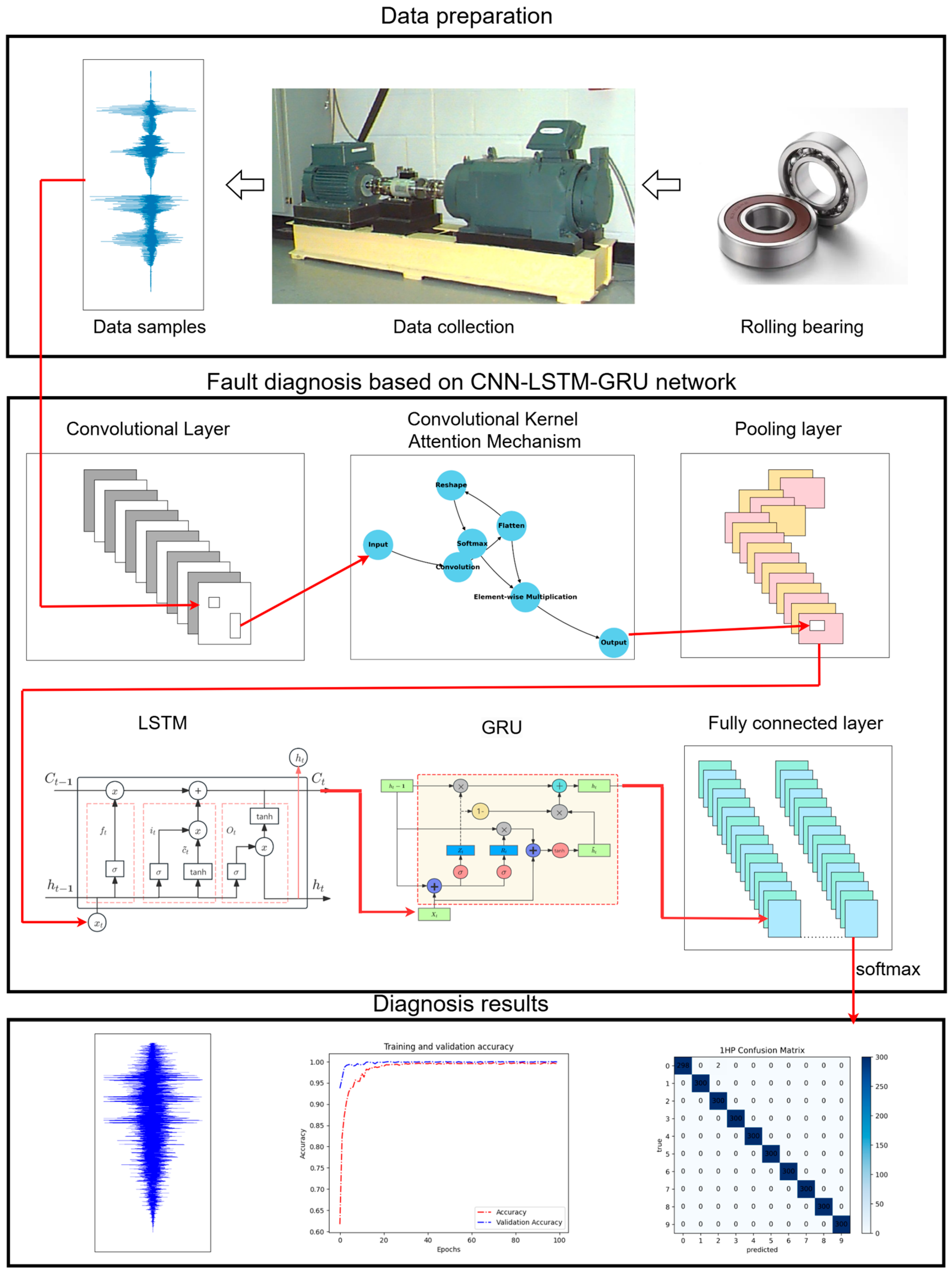
• To provide the diagnostic model with a stable time series prediction ability and an efficient comprehensive spatiotemporal feature extraction ability, this study optimizes the network hierarchy structure of a convolutional neural network (CNN) to strengthen the extraction of spatial features. At the same time, it integrates a long short-term memory network (LSTM) network to model the long-term trends of the time series. In addition, a gated recurrent unit (GRU), which efficiently processes medium- and short-length sequences, is introduced to locally fine-tune the long time series, enabling better management and maintenance of the long-term time series prediction results.
• The proposed model was evaluated using comparative experiments. This method can effectively prevent gradient vanishing and data overfitting compared to other models, and has higher robustness, with a comprehensive diagnostic accuracy of 99.34%.

The remainder of this article is organized as follows. Section 2 introduces the basic network of the CNN-LSTM-GRU model. Section 3 presents the CNN-LSTM-GRU model framework. Section 4 presents the validation results and a discussion of the CNN-LSTM-GRU model in stable and noisy environments. Section 5 provides conclusions and future research directions.

2. Related Work

2.1. Convolutional Neural Network (CNN)

CNNs are a variant of multilayer fully connected neural networks, consisting of multiple filtering processes and a classification process. Compared with fully connected networks, CNNs offer superior performance [27] in many engineering applications due to their local connectivity, shared weights, and pooling layers. CNNs enhance spatial feature extraction capabilities through parameter optimization. Its structure is shown in Figure 1.

This layer uses convolutional kernels to gradually perform local convolution operations on input features, and the depth of the output feature map corresponds to the number of convolutional kernels. An example of a convolution operation is as follows:

$${\mathrm{y}}^{\mathrm{l}}={\displaystyle \sum _{\mathrm{i}=1}^{{\mathrm{c}}^{\mathrm{l}-1}}{{\mathrm{w}}^1}_{\mathrm{i},\mathrm{c}}\ast {{\mathrm{x}}^{\mathrm{l}-1}}_{\mathrm{i}}+{{\mathrm{b}}^{\mathrm{l}}}_{\mathrm{i}}}$$

(1)

In this formula, y^l is the weight matrix of the convolution kernel in layer l; c^l−1 is the number of channels in layer l − 1; W¹_i,c is the weight connecting the i th output channel to the c th input channel; x^l−1_i is the output of the i th channel in layer l − 1; b¹_i is the bias term of the first output channel in layer l; and ∗ is the convolution operation.

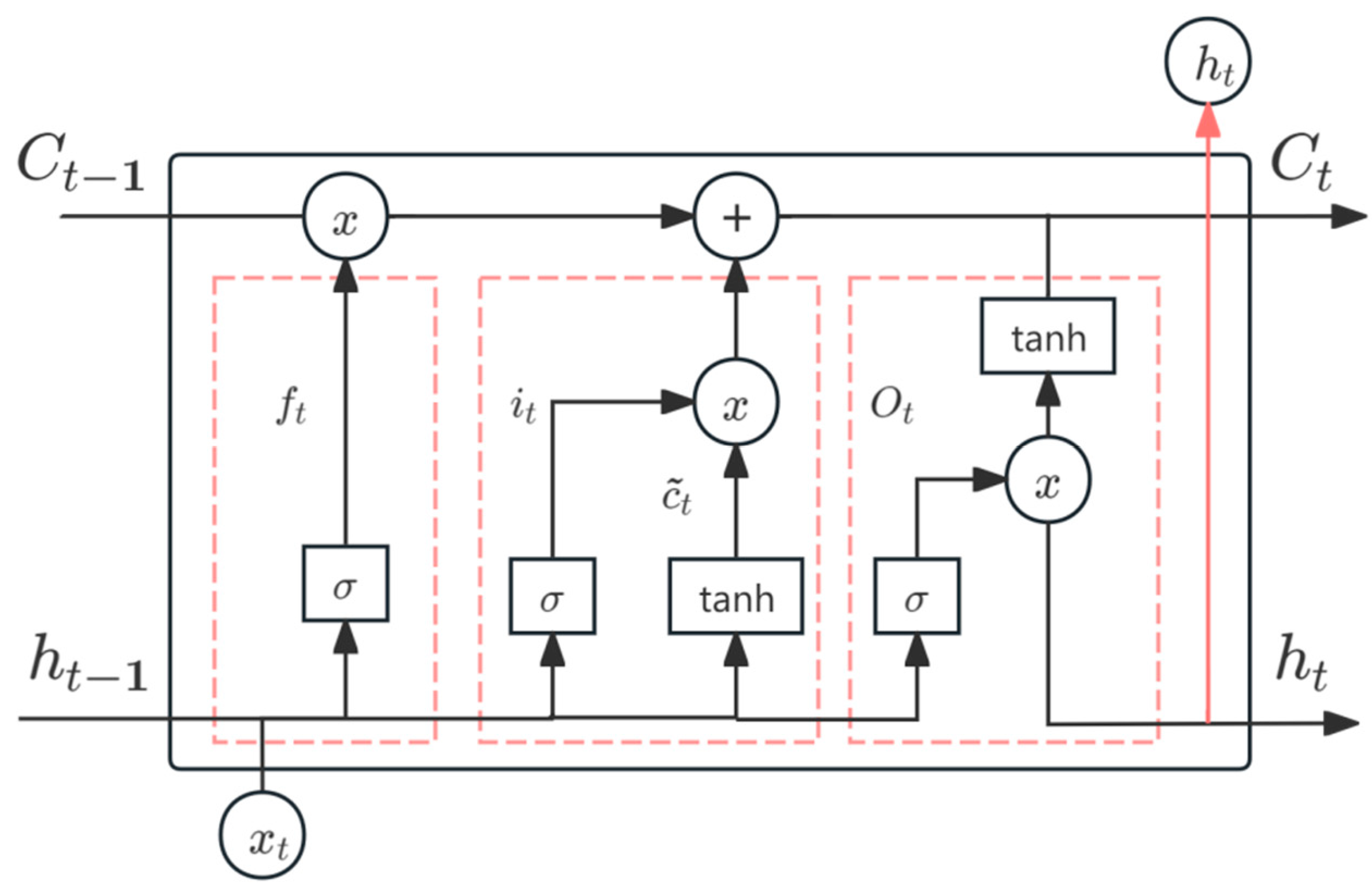
2.2. Long Short-Term Memory (LSTM) Network

The long short-term memory (LSTM) network was jointly proposed by scientists Hochreiter and Schmidhuber. Its structure is shown in Figure 2 according to [28]. An LSTM not only handles time series data, such as bearing vibration signals, but its gating mechanism also captures long-term dependencies; it can automatically extract fault features and adapt to characteristic changes under different working conditions. By using an LSTM, the model is better able to process long-sequence signal data and model long-term trend changes in time series data.

The LSTM network consists of one or more LSTM units used to capture long-term dependencies in time series data. The operations of LSTM units are expressed in Equations (2), (3), (4), (5), and (6), separately.

$${\mathrm{i}}_{\mathrm{t}}=\sigma ({\mathrm{W}}_{\mathrm{i}}\ast [{\mathrm{h}}_{\mathrm{t}-1},{\mathrm{x}}_{\mathrm{t}}]+{\mathrm{b}}_{\mathrm{i}})$$

(2)

$${\mathrm{f}}_{\mathrm{t}}=\sigma ({\mathrm{W}}_{\mathrm{f}}\ast [{\mathrm{h}}_{\mathrm{t}-1},{\mathrm{x}}_{\mathrm{t}}]+{\mathrm{b}}_{\mathrm{f}})$$

(3)

$${\mathrm{o}}_{\mathrm{t}}=\sigma ({\mathrm{W}}_{\mathrm{o}}\ast [{\mathrm{h}}_{\mathrm{t}-1},{\mathrm{x}}_{\mathrm{t}}]+{\mathrm{b}}_{\mathrm{o}})$$

(4)

$${\mathrm{C}}_{\mathrm{t}}={\mathrm{f}}_{\mathrm{t}}\ast {\mathrm{C}}_{\mathrm{t}-1}+{\mathrm{i}}_{\mathrm{t}}\ast \tanh ({\mathrm{W}}_{\mathrm{c}}\ast [{\mathrm{h}}_{\mathrm{t}-1},{\mathrm{x}}_{\mathrm{t}}]+{\mathrm{b}}_{\mathrm{c}})$$

(5)

$${\mathrm{h}}_{\mathrm{t}}={\mathrm{o}}_{\mathrm{t}}\ast \tanh ({\mathrm{C}}_{\mathrm{t}})$$

(6)

In these formulas, i_t, f_t, and o_t are the activation values of the input gate, forgetting gate, and output gate at time step t; C_t−1, C_t, and h_t are the cell state at the previous t − 1, the cell state at current t, and the hidden state at current t, respectively; $\sigma$ is the activation function; W_i, W_f, W_o, and W_c are the weight matrices of the input gate, forgetting gate, output gate, and cell states, respectively; [h_t−1, x_t] connects the hidden state of the previous moment h_t−1 and the input x_t of the current moment into a vector; b_i, b_f, b_o, and b_C represent biased vectors of the input gate, forgetting gate, output gate, and cell states, respectively; tanh is a hyperbolic tangential activation function; and tanh (C_t) applies a hyperbolic tangent activation function to the current cell state.

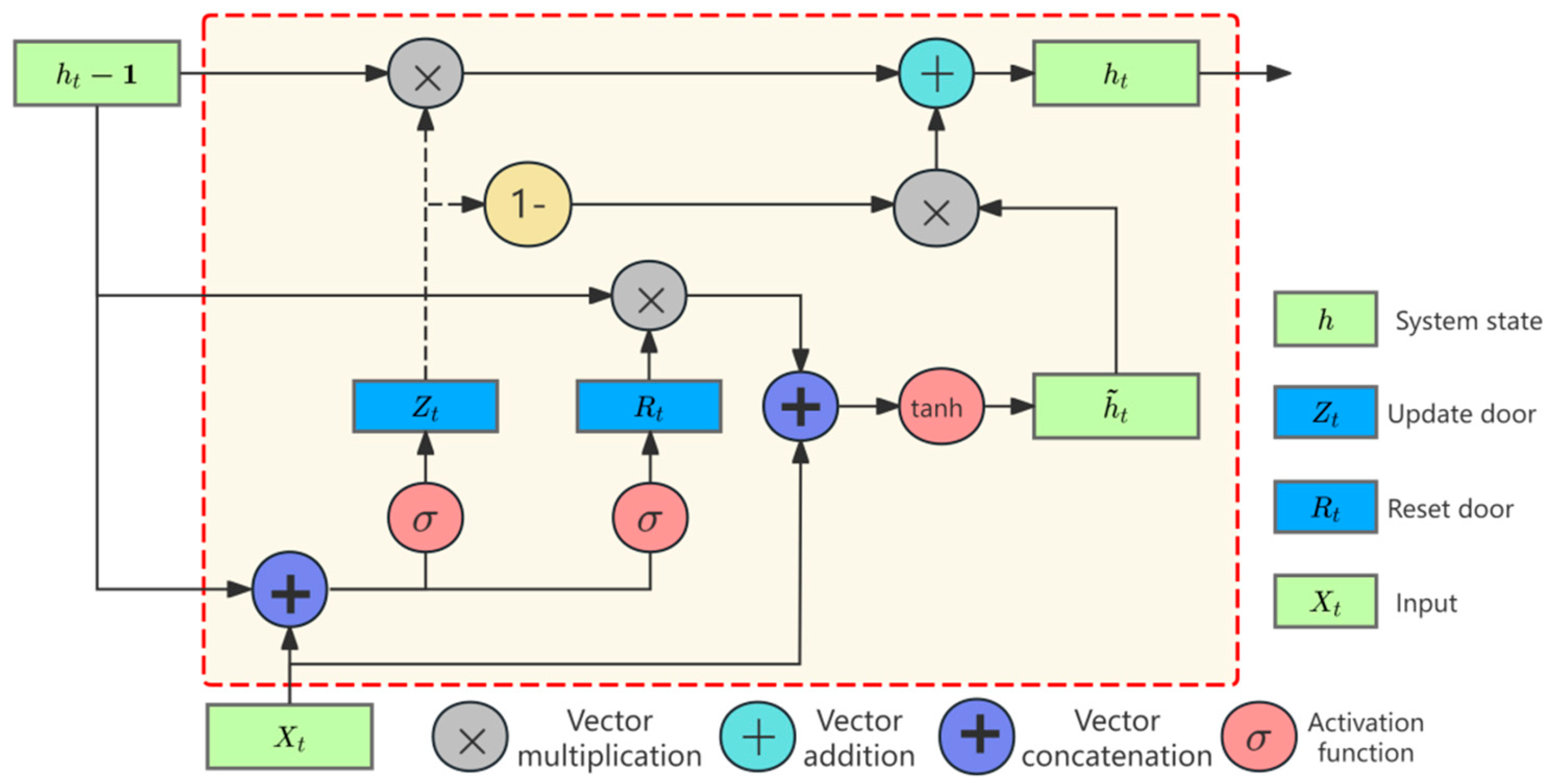
2.3. Gated Recurrent Unit (GRU)

The gated recurrent unit (GRU) is a modified RNN. Similar to an LSTM, a GRU manages and maintains short time dependencies through the gating mechanism, but its structure is more concise than an LSTM [29]. A GRU is used to manage and maintain part of the prediction results to achieve local fine-tuning of the time series data, and its structure is shown in Figure 3.

The input and output of a GRU are similar to an LSTM. The GRU formulas are detailed in Equations (7)–(10):

$${\mathrm{Z}}_{\mathrm{t}}=\sigma ({\mathrm{W}}_{\mathrm{z}}\cdot [{\mathrm{h}}_{\mathrm{t}-1},{\mathrm{x}}_{\mathrm{t}}]+{\mathrm{b}}_{\mathrm{z}})$$

(7)

$${\mathrm{r}}_{\mathrm{t}}=\sigma ({\mathrm{W}}_{\mathrm{r}}\cdot [{\mathrm{h}}_{\mathrm{t}-1},{\mathrm{x}}_{\mathrm{t}}]+{\mathrm{b}}_{\mathrm{r}})$$

(8)

$${\tilde{\mathrm{h}}}_{\mathrm{t}}=\tanh ({\mathrm{W}}_{\mathrm{h}}\cdot [{\mathrm{r}}_{\mathrm{t}}\ast {\mathrm{h}}_{\mathrm{t}-1},{\mathrm{x}}_{\mathrm{t}}]+{\mathrm{b}}_{\mathrm{h}})$$

(9)

$${\mathrm{h}}_{\mathrm{t}}=(1-{\mathrm{Z}}_{\mathrm{t}})\ast {\mathrm{h}}_{\mathrm{t}-1}+{\mathrm{Z}}_{\mathrm{t}}\ast \mathrm{h}$$

(10)

Here, z_t is the update gate; r_t is the reset gate; ${\tilde{\mathrm{h}}}_{\mathrm{t}}$ is the candidate hidden state; h_t is the hidden state of GRU; $\sigma$ is the activation function; W_z, W_r, and W_h are the weight matrix of update gate, reset gate, and candidate hidden state; [h_t−1, x_t] connect the hidden state h_t−1 and the current moment into a vector; [r_t ∗ h_t−1, x_t] is the hidden state of the previous moment under the control of the reset gate-1 with the current input x_t into a vector; b_z, b_r, and b_h are the bias vectors of the update gate, reset gate, and candidate hidden state, respectively.

3. Fault Diagnosis Model for Rolling Bearings

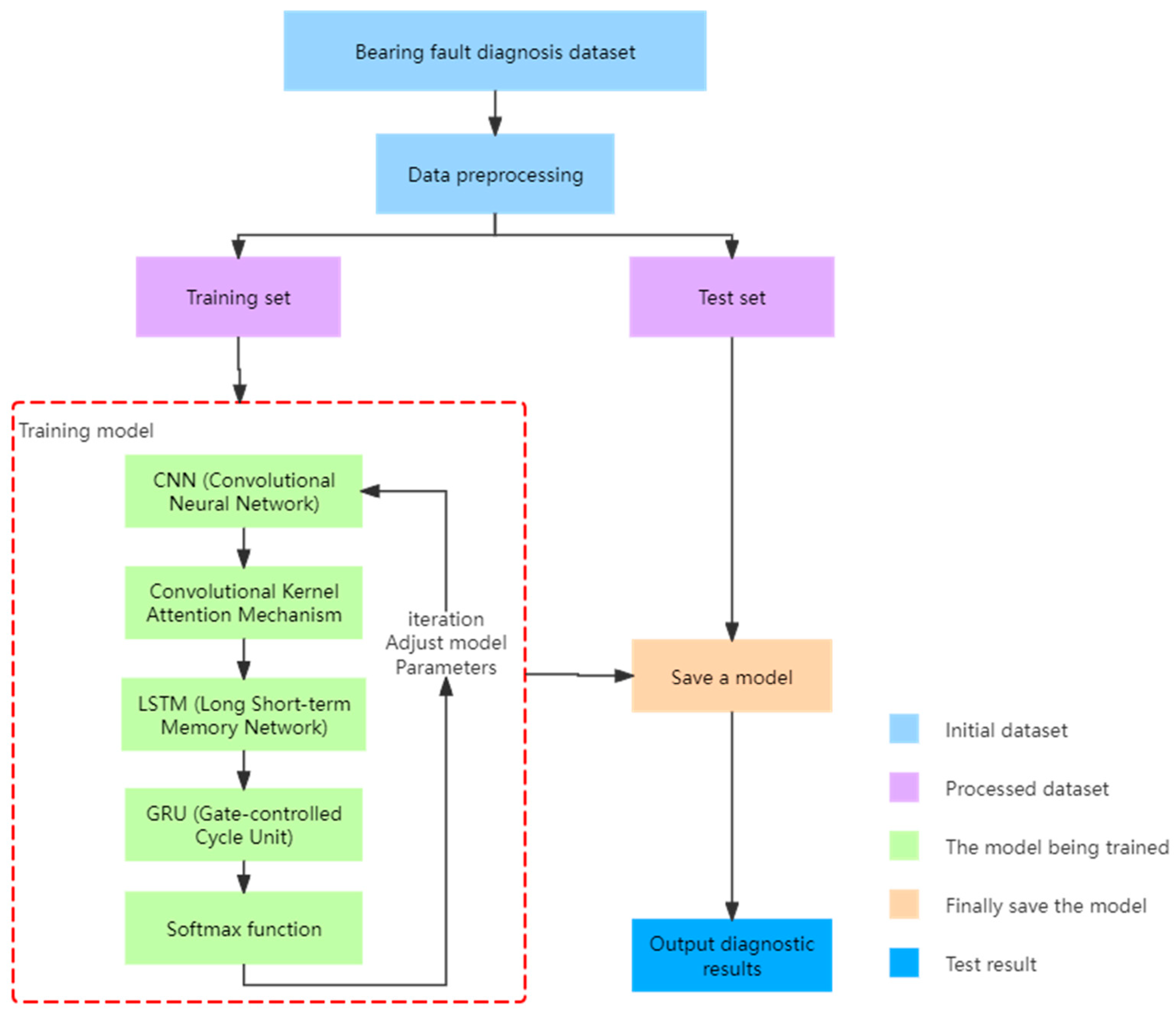
3.1. A Bearing Diagnosis Model Based on a CNN-LSTM-GRU Model

To ensure that the model has stable temporal prediction performance and to improve its spatial and temporal feature extraction ability, a CNN-LSTM-GRU diagnosis method is designed in this study. Its architecture is shown in Figure 4. The final output data from left to right are diagnosis output results, model accuracy curve, and confusion matrix. The model takes the optimized convolutional neural network (CNN) as the core and introduces a convolutional kernel attention mechanism to enhance the model’s ability to extract spatial features in the single-sample feature extraction process. Given that bearing fault diagnosis is a changing trend of long-term time series data, this study introduces a long short-term memory (LSTM) network with an excellent long-term time series feature extraction ability to improve fault diagnosis performance and model long-term trend changes [30] in time series prediction performance. Due to the limitations of the LSTM network in capturing the trends of short- and medium-length time series data, this study further integrates the gated recurrent unit (GRU) to locally fine-tune [31] the prediction results of long time series, thereby enhancing the diagnostic capability of the diagnostic model.

The structure hierarchy of the CNN-LSTM-GRU model is relatively complex. Its design principle is to enhance diagnostic accuracy by improving computational complexity and covering the signal input layer, CNN convolution layer, convolution core concentration mechanism, pooling layer, LSTM layer, GRU layer, and classification output layer. During the study design phase, the model achieves the highest improvement in test accuracy, which is based on the importance of fault diagnosis and the need for high precision. For many industrial systems, especially those in safety-critical areas such as aerospace, healthcare, and energy production, accurate fault diagnosis is crucial, even if it results in a modest increase in computational complexity.

As shown in Figure 5, the diagnostic process first involves a preprocessing step of the rolling bearing dataset. The input layer of the convolutional neural network (CNN) receives the preprocessed data, where the convolution kernel is responsible for extracting the local features of the signal. Subsequently, the normalized layer standardizes the output of the convolution layer, while the ReLU activation function and batch normalization technique further enhance the robustness of the training process. After multiple rounds of convolution operation and batch normalization processing, the data are transmitted to the long short-term memory (LSTM) network layer to realize the extraction of long-term timing-dependent features. Next, the data pass through the gated recurrent unit (GRU) layer to overcome the limitations of the LSTM network in processing short time series data. After the output of the GRU layer is fully connected and flattened, the Softmax activation function completes the fault classification task in the output layer. Ultimately, the model’s performance on the test set was evaluated through test validation.

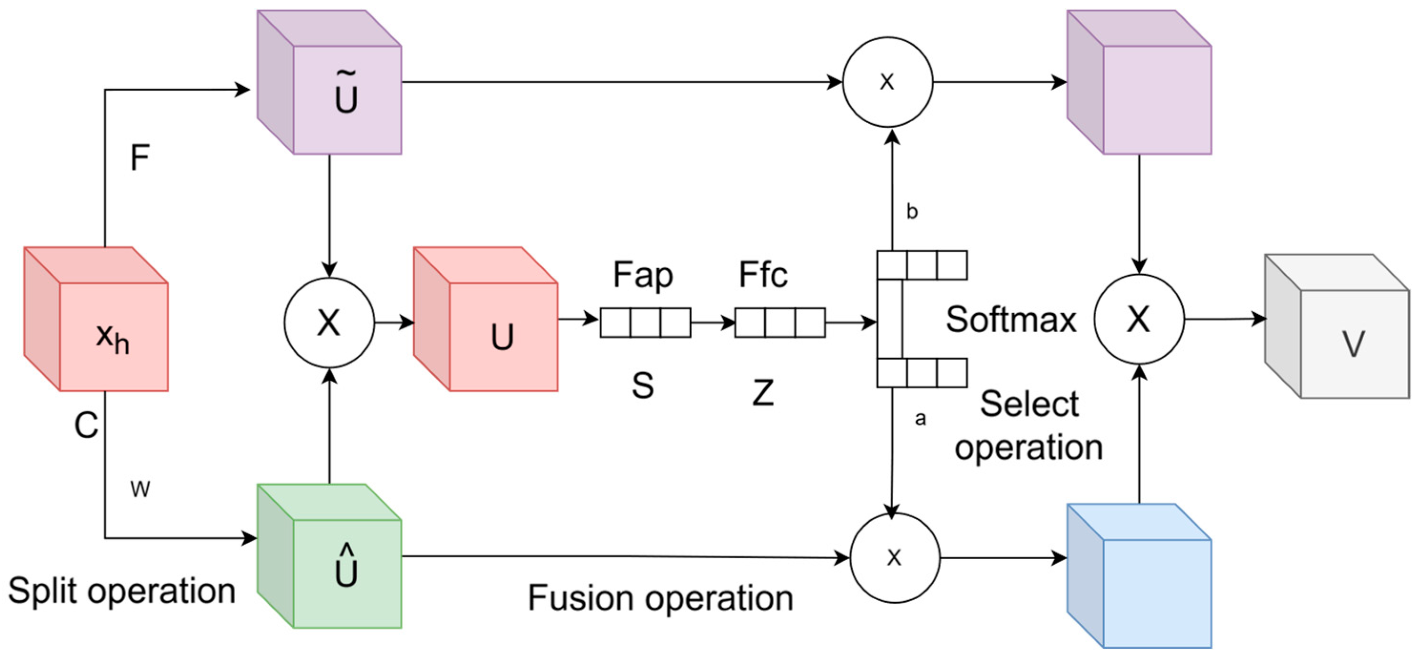
3.2. Convolutional Kernel Attention Mechanism

The selective kernel coil integrates the attention and gating mechanism based on the convolution kernel of different sizes, and processes the temporal information flow to change the input [32]. Figure 6 shows the structure of the convolution kernel attention mechanism. After the feature diagram X is introduced, the convolution kernel specifications are $\tilde{\mathrm{U}}$(3 × 3) and $\hat{\mathrm{U}}$(5 × 5), and the final feature diagram U and V contain different scale information. According to the feature diagram U, the process is shown in Equation (11) as follows:

$$\mathrm{U}=\tilde{\mathrm{U}}+\hat{\mathrm{U}}$$

(11)

3.3. Softmax Activation Function

The prediction probability [33] for each category is completed using the Softmax activation function. Given a K-dimensional input vector z = [z1, z2, …, zK], the Softmax function maps it to the other K-dimensional output vector σ(z) = [σ(z)1, σ(z)2, …, σ(z)K], where each element is calculated as shown in Equation (12):

$$\sigma {(\mathrm{z})}_{\mathrm{j}}={\displaystyle \frac{{\mathrm{e}}^{\mathrm{zj}}}{{\displaystyle {\sum }_{\mathrm{k}=1}^{\mathrm{k}}{\mathrm{e}}^{\mathrm{zk}}}}}\hspace{1em}{\displaystyle {\displaystyle \mathrm{for}}}\hspace{1em}\mathrm{j}=1,\dots ,\mathrm{K}$$

(12)

Here, σ(z)_j represents the output of the Softmax function; z is the input vector; j is the index of the output vector; and e^zj and ezk are the exponential function values of the j and k elements in the input vector z. The denominator is the sum of the exponential function values of all elements, used for normalization to ensure that the sum of all elements in the output vector is 1.

4. Experimental Study

In this study, the CNN-LSTM-GRU model was applied to a CWRU rolling bearing dataset and conducted comparative experiments of steady-state analysis and anti-noise analysis with several deep learning methods. In addition, five-fold cross-validation of accuracy was performed to evaluate its performance. The deep learning models used for comparison include the convolutional neural network-long short-term memory network (CNN-LSTM), long short-term memory (LSTM) network, convolutional neural network (CNN), deep neural network (DNN), back propagation neural network (BPNN), and random forest algorithm. The hardware and software configuration information of the tools used in the laboratory include the following: the operating system is Windows 10; the processor model is Intel (Santa Clara, CA, USA) Core i5-9300H; the memory capacity is 16 GB; the graphics card is NVIDIA (Santa Clara, CA, USA) GeForce GTX 1650; the programming language Python is 3.10.0, and the deep learning framework version is tensorflow 2.17.0.

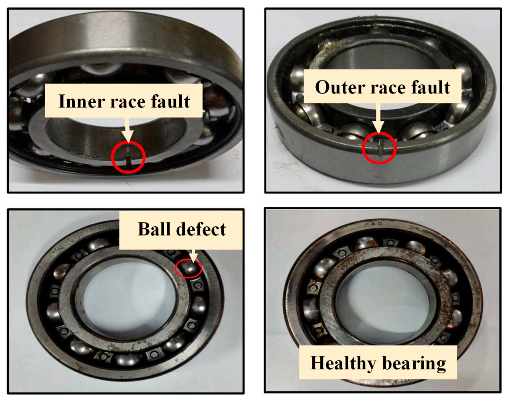
4.1. Introduction to the CWRU Dataset

The dataset used in this study was constructed by researchers from the Case Western Reserve University School of Mechanical and Space Engineering to explore mechanical bearing state monitoring and fault diagnosis monitoring techniques. The structural layout of the test device experimental platform is shown in Figure 7, which includes a Reliance motor with 2 horsepower on the left, a dynamometer on the right, and a torque sensor/encoder in the middle. Using electrical discharge machining technology, this study replicated bearing failure damage diameters with dimensions of 0.178 mm, 0.356 mm, and 0.533 mm separately.

The bearings used in the experiment were deep groove ball bearings from 6205-2RS JEM SKF. In the dataset, the motor speed is 1797 r/min, 1772 r/min, 1750 r/min, and 1730 r/min, corresponding to four working conditions of 0 kW, 0.735 kW, 1.47 kW, and 2.205 kW, respectively. For each working condition, the fault data of the rolling body, inner ring, and outer ring are collected, and these data reflect the characteristics of different damage diameters. The bearing is damaged as shown in Figure 8. When selecting the outer circle data, the damage position is set at the 6 o’clock direction, based on which of the four datasets are constructed, with each corresponding to different working conditions. Each condition contains nine bearing fault states and one normal condition, with a total of 10 class labels. The training set of each category label consists of 700 samples, and the test set contains 300 samples. The ratio of the training set to the test set is maintained at 7:3. Detailed dataset information is shown in

Table 1. Dataset description.

Label	Damage Location	Damage Diameter	Training Set	Test Set
0	Rolling element damage	0.178	700	300
1	Rolling element damage	0.356	700	300
2	Rolling element damage	0.533	700	300
3	Inner ring damage	0.178	700	300
4	Inner ring damage	0.356	700	300
5	Inner ring damage	0.533	700	300
6	Outer ring damage	0.178	700	300
7	Outer ring damage	0.356	700	300
8	Outer ring damage	0.533	700	300
9	Normal	0.000	700	300

.

4.2. Experimental Comparison and Result Analysis

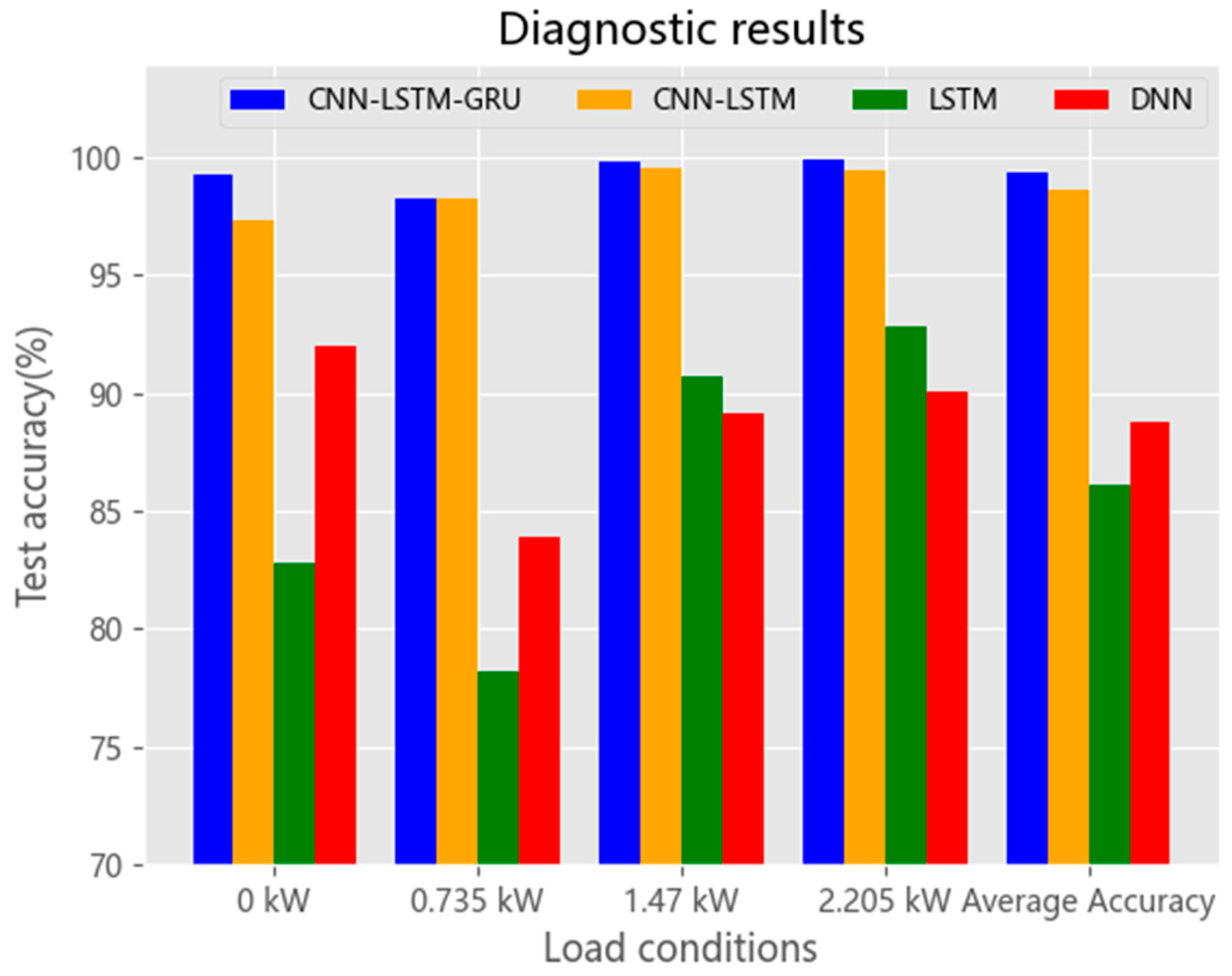
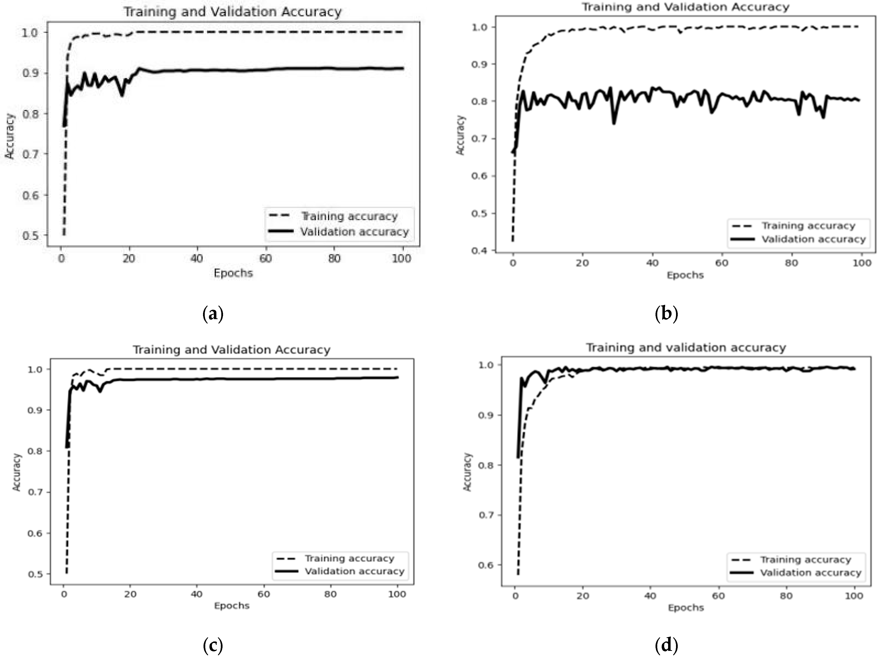
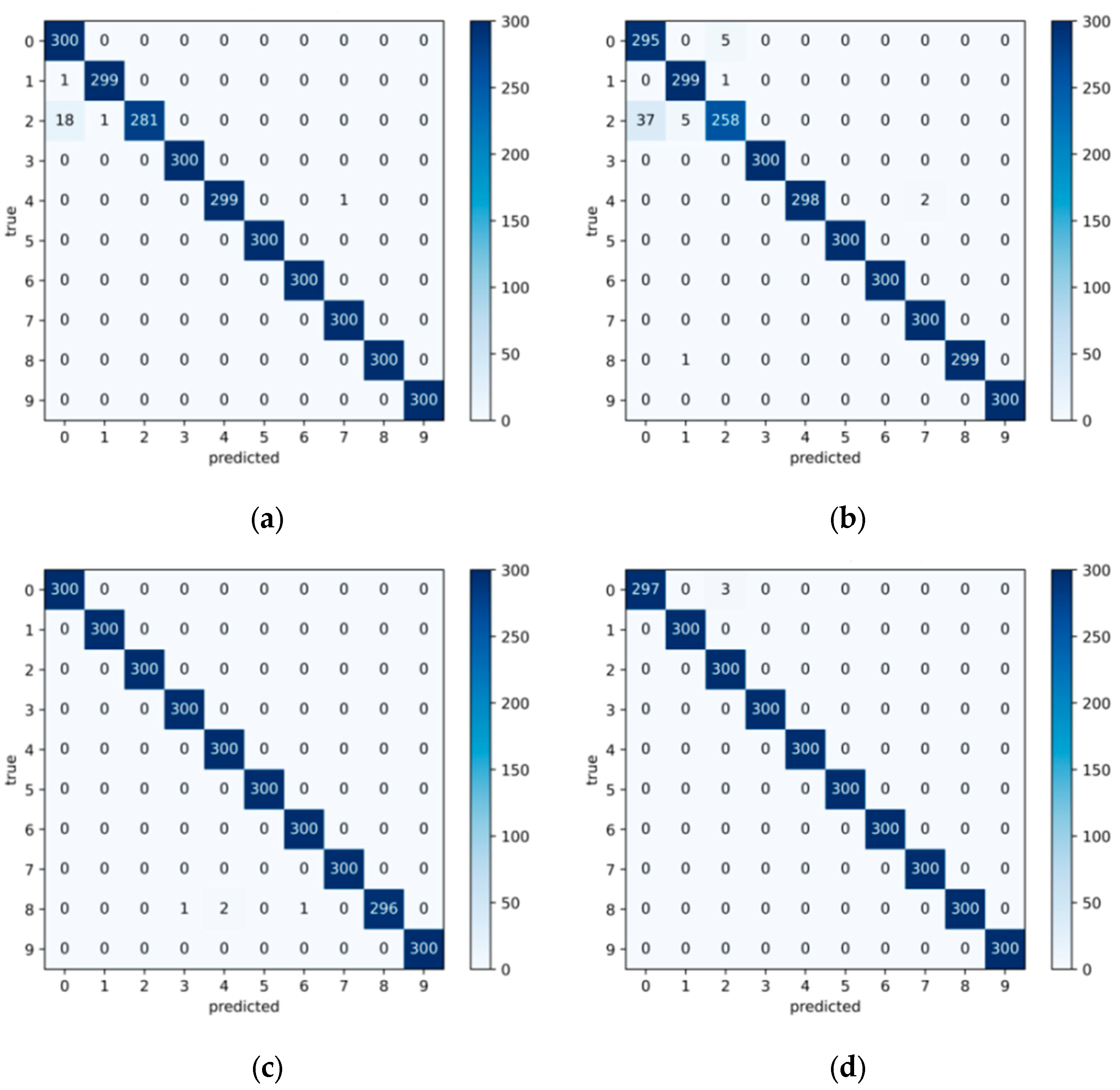
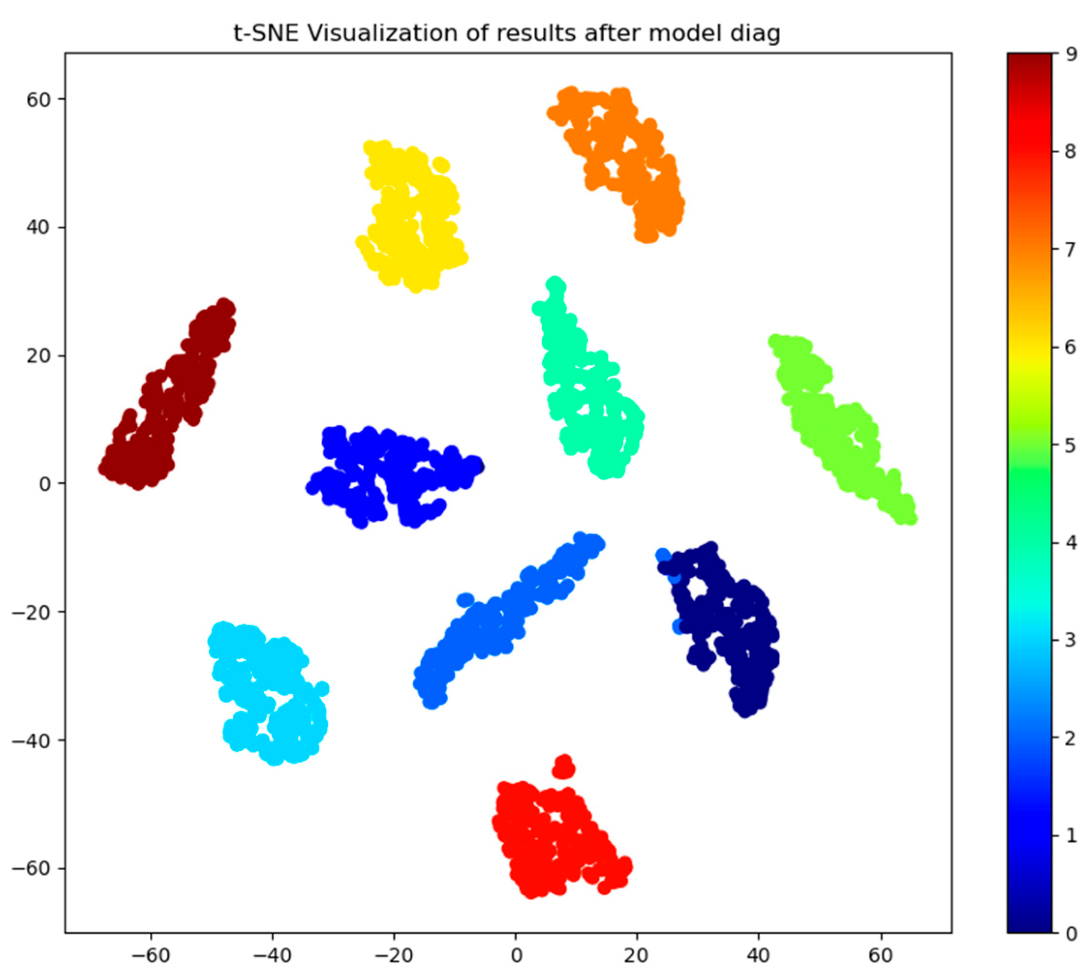
4.2.1. Diagnosis Comparison Experiments Under a Stable Environment

The experiment used the dataset introduced above and the CNN-LSTM-GRU model to verify the dataset under different loads. The number of iterations of each dataset was 100, and the average results of the accuracy using five-fold cross-validation under different working conditions are shown in

Table 2. Diagnosis results of CNN-LSTM-GRU model under different operating conditions.

Load	Accuracy	Number of Iterations
0 kW	99.29%	100
0.735 kW	98.29%	100
1.47 kW	99.86%	100
2.205 kW	99.90%	100

:

The results show that the model achieved more than 98% accuracy on datasets with 0 kW, 0.735 kW, 1.47 kW, and 2.205 kW, and exceeded 99% accuracy with 0 kW, 1.47 kW, and 2.205 kW. In the load condition of 0.735 kW, there is neither simplicity of the no-load state nor significant amplification of the features in the high-load state. In this case, the vibration signal caused by the fault is prone to interference by other factors, resulting in superposition of the load-induced normal vibration and the fault vibration, thus blurring the fault characteristics. Nevertheless, the average accuracy of this study method still reached 99.34%. To confirm the superiority of the model, CWRU experimental data were used as the standard bearing vibration dataset, and the model was compared with the conventional CNN-LSTM model, LSTM model, and DNN model under the same experimental conditions to prove the comprehensive long-sequence spatiotemporal feature extraction ability of the model. The specific comparison results are shown in

Table 3. Diagnosis results of different models under different operating conditions.

Model	Load				Average Accuracy
	0 kW	0.735 kW	1.47 kW	2.205 kW
CNN-LSTM-GRU	99.29%	98.29%	99.86%	99.90%	99.34%
CNN-LSTM	97.36%	98.27%	99.53%	99.43%	98.65%
LSTM	82.77%	78.23%	90.71%	92.82%	86.13%
DNN	92.01%	83.91%	89.11%	90.10%	88.78%

and Figure 9.

Table 2 shows that the CNN-LSTM-GRU model improved by 0.67% over the conventional CNN-LSTM model under all conditions. Compared with LSTM and DNN neural networks, the accuracy of the model is improved by 13.19% and 10.54%, respectively, with the greatest improvement noted under the 0 kW condition. It can be observed that the model performs well in predicting stable time series and maintains a high ability for comprehensive spatiotemporal feature extraction. Moreover, the training and test accuracy curves of the four models under zero load are presented in Figure 10, and the confusion matrix of the CNN-LSTM-GRU model for each condition in the dataset is shown in Figure 11.

Bearing feature extraction results are shown in t-SNE plots in Figure 12 and Figure 13. Fault types, labeled from 0 to 9 in Table 1, are visualized in Figure 12 using t-SNE. After being processed by the fault diagnosis model proposed in this paper, as shown in Figure 13, different types of faults present clear clustered distributions in low dimensional space, making observation and analysis easier.

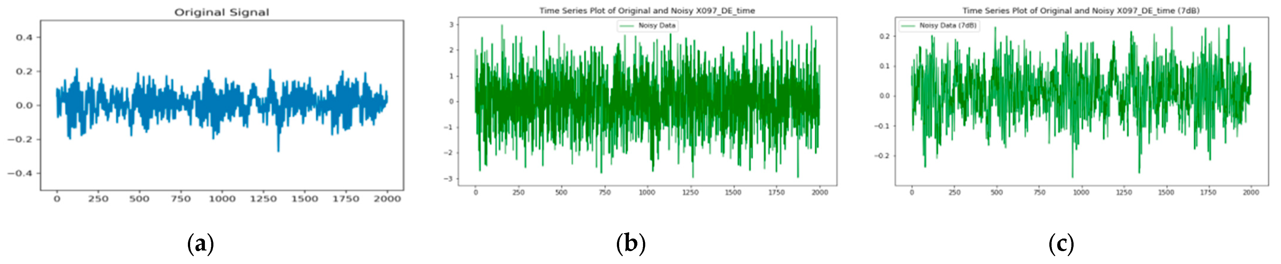
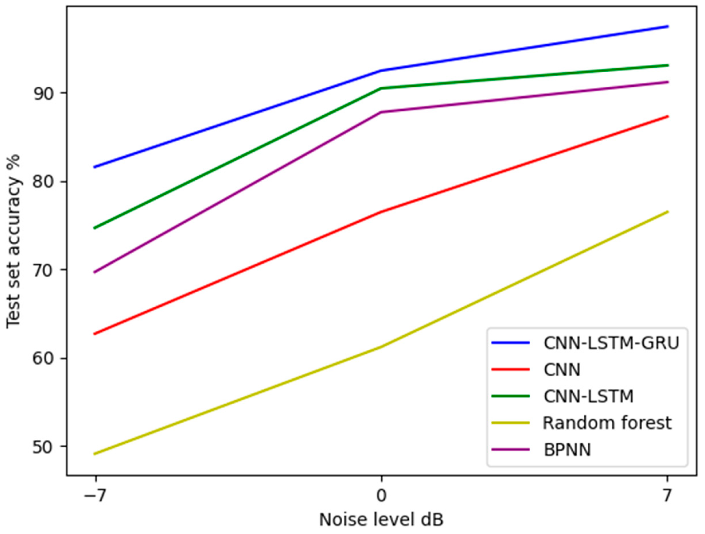
4.2.2. Comparative Experiment of Diagnosis in a Noisy Environment

To verify the generalization ability of the improved CNN-LSTM-GRU model under strong noise and variable load conditions, the model was tested for fault diagnosis accuracy after superimposing noise on the bearing vibration signal. The SNR can be calculated using Equation (13).

$$\mathrm{SNR}=10\cdot \log 10({\displaystyle \frac{{\mathrm{P}}_{\mathrm{signal}}}{{\mathrm{P}}_{\mathrm{nois}}}})$$

(13)

The formula for calculating the SNR is based on the average power P of the signal, where P_signal represents the power of the signal, and P_noise is the power of the noise. Using the normal bearing sample from the dataset as an example, the study shows the original signal, the signal with 0 dB noise, and the signal with 7 dB noise, as shown in Figure 14.

The CNN-LSTM-GRU model is compared with the traditional CNN, CNN-LSTM, BPNN, and random forest models. Under the same experimental conditions, −7 db, 0 dB, and 7 dB of noise are separately added for fault diagnosis. To more intuitively compare different algorithms under different noise conditions, the average value of diagnostic accuracy is obtained using five-fold cross-validation. The results are shown in

Table 4. Comparison of test accuracies of different algorithms and different levels of noise.

Algorithm	CNN-LSTM-GRU	CNN-LSTM	CNN	BPNN	Random Forest
−7 dB	81.6%	74.7%	62.7%	69.7%	49.1%
0 dB	92.5%	90.5%	76.5%	87.8%	61.2%
7 dB	97.2%	93.1%	87.3%	91.2%	76.5%

and Figure 15.

The fault diagnosis rate of CNN-LSTM-GRU under noise levels ranging from −7 dB to 7 dB is better than other models, indicating that the model can effectively solve the interference of strong noise and learn more effective fault features from complex vibration signals. Under a relatively strong interference of −7 dB, the fault diagnosis rate of the CNN-LSTM-GRU model reached 81.6%, which is 6.9% higher than CNN-LSTM, and shows improvements of 11.9%, 18.9%, and 32.5% compared with BPNN, CNN, and random forest, respectively. To evaluate the model’s robustness to noise, the experimental results of bearing fault diagnosis under 0 dB background noise were compared. The accuracy curve and confusion matrix are shown in Figure 16 and Figure 17, respectively.

5. Conclusions

To ensure stable time series prediction performance of the diagnostic model while ensuring efficient comprehensive spatiotemporal feature extraction, this study developed the CNN-LSTM-GRU method. By optimizing convolutional neural networks (CNNs) and integrating long short-term memory (LSTM) networks, the ability to extract comprehensive spatiotemporal features has been enhanced. In addition, to further optimize the time prediction performance of the model, a gated recurrent unit (GRU) is integrated to locally fine-tune the long-term time prediction results to improve diagnostic performance. Although overall network complexity has increased, it has also increased the contribution of important information while eliminating the interference of irrelevant features. The model’s superiority was validated on a CWRU dataset, demonstrating its ability maintain high diagnostic accuracy in noisy environments, making it better suited for complex industrial applications.

The CNN-LSTM-GRU model developed in this article effectively improves the accuracy and stability of rolling bearing fault diagnosis, contributing to better monitoring and fault warning of rolling bearings in industrial equipment. This, in turn, plays a positive role in the broader field of industrial production. In the future, improving the generalization ability of deep learning models will become a key research area. To expand the application scope of these models, this method will be further explored using datasets such as MFPT, PU, and CWRU under different operating conditions.

References

1. Desnica, E.; Ašonja, A.; Radovanović, L.; Palinkaš, I.; Kiss, I. Selection, Dimensioning and Maintenance of Roller Bearings. In 31st International Conference on Organization and Technology of Maintenance (OTO 2022); Blažević, D., Ademović, N., Barić, T., Cumin, J., Desnica, E., Eds.; OTO 2022. Lecture Notes in Networks and Systems; Springer: Cham, Switzerland, 2023; Volume 592. [Google Scholar] [CrossRef]
2. Pastukhov, A.; Timashov, E.; Stanojević, D. Temperature Conditions and Diagnostics of Bearings. Appl. Eng. Lett. 2023, 8, 45–51. [Google Scholar] [CrossRef]
3. Shi, R.; Wang, B.; Wang, Z.; Liu, J.; Feng, X.; Dong, L. Research on Fault Diagnosis of Rolling Bearings Based on Variational Mode Decomposition Improved by the Niche Genetic Algorithm. Entropy 2022, 24, 825. [Google Scholar] [CrossRef] [PubMed]
4. Wang, X.; Hua, T.; Xu, S.; Zhao, X. A Novel Rolling Bearing Fault Diagnosis Method Based on BLS and CNN with Attention Mechanism. Machines 2023, 11, 279. [Google Scholar] [CrossRef]
5. Lee, S.; Kim, S.; Kim, S.J.; Lee, J.; Yoon, H.; Youn, B.D. Revolution and peak discrepancy-based domain alignment method for bearing fault diagnosis under very low-speed conditions. Expert Syst. Appl. 2024, 251, 124084. [Google Scholar] [CrossRef]
6. Kulevome, D.K.B.; Wang, H.; Cobbinah, B.M.; Mawuli, E.S.; Kumar, R. Effective time-series Data Augmentation with Analytic Wavelets for bearing fault diagnosis. Expert Syst. Appl. 2024, 249 Pt A, 123536. [Google Scholar] [CrossRef]
7. Ma, H.; Li, S.; Lu, J.; Gong, S.; Yu, T. Impulsive wavelet based probability sparse coding model for bearing fault diagnosis. Measurement 2022, 194, 110969. [Google Scholar] [CrossRef]
8. Biao, H.; Qin, Y.; Luo, J.; Yang, W.; Xu, L. Impulse feature extraction via combining a novel voting index and a variational model penalized by center frequency constraint. Mech. Syst. Sig. Process. 2023, 186, 109889. [Google Scholar] [CrossRef]
9. Yin, L.; Wang, Z. Bi-level binary coded fully connected classifier based on residual network 50 with bottom and deep level features for bearing fault diagnosis. Eng. Appl. Artif. Intell. 2024, 133 Pt D, 108342. [Google Scholar] [CrossRef]
10. Wang, X.; Jiang, H.; Wu, Z.; Yang, Q. Adaptive variational autoencoding generative adversarial networks for rolling bearing fault diagnosis. Adv. Eng. Inf. 2023, 56, 102027. [Google Scholar] [CrossRef]
11. Shi, H.; Guo, L.; Tan, S.; Bai, X. Rolling bearing initial fault detection using long short-term memory recurrent network. IEEE Access 2019, 7, 171559–171569. Available online: https://ieeexplore.ieee.org/document/8905994 (accessed on 9 January 2024). [CrossRef]
12. Ruan, D.; Wang, J.; Yan, J.; Gühmann, C. CNN parameter design based on fault signal analysis and its application in bearing fault diagnosis. Adv. Eng. Inform. 2023, 55, 101877. [Google Scholar] [CrossRef]
13. Zhang, S.; Qiu, T. Semi-supervised LSTM ladder autoencoder for chemical process fault diagnosis and localization. Chem. Eng. Sci. 2022, 251, 117467. [Google Scholar] [CrossRef]
14. Jia, F.; Lei, Y.; Lu, N.; Xing, S. Deep normalized convolutional neural network for imbalanced fault classification of machinery and its understanding via visualization. Mech. Syst. Sig. Process. 2018, 110, 349–367. [Google Scholar] [CrossRef]
15. Zhang, W.; Li, C.; Peng, G.; Chen, Y.; Zhang, Z. A deep convolutional neural network with new training methods for bearing fault diagnosis under noisy environment and different working load. Mech. Syst. Sig. Process. 2018, 100, 439–453. [Google Scholar] [CrossRef]
16. Grezmak, J.; Zhang, J.; Wang, P.; Loparo, K.A.; Gao, R.X. Interpretable convolutional neural network through layer-wise relevance propagation for machine fault diagnosis. IEEE Sens. J. 2020, 20, 3172–3181. Available online: https://ieeexplore.ieee.org/document/8930493 (accessed on 9 January 2024). [CrossRef]
17. Yu, W.; Zhao, C. Online Fault Diagnosis for Industrial Processes with Bayesian Network-Based Probabilistic Ensemble Learning Strategy. IEEE Trans. Autom. Sci. Eng. 2019, 16, 1922–1932. [Google Scholar] [CrossRef]
18. Meng, Z.; Cao, W.; Sun, D.; Li, Q.; Ma, W.; Fan, F. Research on fault diagnosis method of MS-CNN rolling bearing based on local central moment discrepancy. Adv. Eng. Inform. 2022, 54, 101797. [Google Scholar] [CrossRef]
19. Yu, W.; Zhao, C. Broad Convolutional Neural Network Based Industrial Process Fault Diagnosis with Incremental Learning Capability. IEEE Trans. Ind. Electron. 2020, 67, 5081–5091. [Google Scholar] [CrossRef]
20. Da, T.N.; Thanh, P.N.; Cho, M.-Y. Novel cloud-AIoT fault diagnosis for industrial diesel generators based hybrid deep learning CNN-BGRU algorithm. Internet Things 2024, 26, 101164. [Google Scholar] [CrossRef]
21. Zhao, H.; Sun, S.; Jin, B. Sequential fault diagnosis based on LSTM neural network. IEEE Access 2018, 6, 12929–12939. Available online: https://ieeexplore.ieee.org/document/8272354 (accessed on 10 January 2024). [CrossRef]
22. Chadha, G.S.; Panambilly, A.; Schwung, A.; Ding, S.X. Bidirectional deep recurrent neural networks for process fault classification. ISA Trans. 2020, 106, 330–342. [Google Scholar] [CrossRef] [PubMed]
23. Yu, W.; Zhao, C.; Huang, B.; Xie, M. An Unsupervised Fault Detection and Diagnosis with Distribution Dissimilarity and Lasso Penalty. IEEE Trans. Control Syst. Technol. 2024, 32, 767–779. [Google Scholar] [CrossRef]
24. Zhao, B.; Cheng, C.; Peng, Z.; Dong, X.; Meng, G. Detecting the early damages in structures with nonlinear output frequency response functions and the CNN-LSTM model. IEEE Trans. Instrum. Meas. 2020, 69, 9557–9567. Available online: https://ieeexplore.ieee.org/document/9130164 (accessed on 10 January 2024). [CrossRef]
25. Zhao, S.; Duan, Y.; Roy, N.; Zhang, B. A deep learning methodology based on adaptive multiscale CNN and enhanced highway LSTM for industrial process fault diagnosis. Reliab. Eng. Syst. Saf. 2024, 249, 110208. [Google Scholar] [CrossRef]
26. Song, B.; Liu, Y.; Fang, J.; Liu, W.; Zhong, M.; Liu, X. An optimized CNN-BiLSTM network for bearing fault diagnosis under multiple working conditions with limited training samples. Neurocomputing 2024, 574, 127284. [Google Scholar] [CrossRef]
27. Lecun, Y.; Bengio, Y.; Hinton, G. Deep learning. Nature 2015, 521, 436. [Google Scholar] [CrossRef]
28. Hochreiter, S.; Schmidhuber, J. Long Short-Term Memory. Neural Comput. 1997, 9, 1735–1780. [Google Scholar] [CrossRef]
29. Liu, J.; Wu, C.; Wang, J. Gated recurrent units based neural network for time heterogeneous feedback recommendation. Inf. Sci. 2018, 423, 50–65. [Google Scholar] [CrossRef]
30. Gao, D.; Zhu, Y.; Ren, Z.; Yan, K.; Kang, W. A novel weak fault diagnosis method for rolling bearings based on LSTM considering quasi-periodicity. Knowl.-Based Syst. 2021, 231, 107413. [Google Scholar] [CrossRef]
31. Andermatt, S.; Pezold, S.; Amann, M.; Cattin, P.C. Multi-dimensional Gated Recurrent Units for Automated Anatomical Landmark Localization. arXiv 2017, arXiv:1708.02766. [Google Scholar] [CrossRef]
32. Shan, X.; Ma, T.; Shen, Y.; Li, J.; Wen, Y. KAConv: Kernel attention convolutions. Neurocomputing 2022, 514, 477–485. [Google Scholar] [CrossRef]
33. Martins, A.F.T.; Astudillo, R.F. From Softmax to Sparsemax: A Sparse Model of Attention and Multi-Label Classification. arXiv 2016, arXiv:1602.02068. [Google Scholar] [CrossRef]
Figure 1. Convolutional neural network structure.
Machines 12 00927 g001
Figure 2. LSTM neuron structure.it, ft, and ot are the activation values of the input gate, forgetting gate, and output gate at time step t.
Machines 12 00927 g002
Figure 3. GRU gated cycle cell structure.
Machines 12 00927 g003
Figure 4. A bearing diagnosis model based on the CNN-LSTM-GRU model.
Machines 12 00927 g004
Figure 5. Flow chart of conventional rolling fault diagnosis based on the CNN-LSTM-GRU model.
Machines 12 00927 g005
Figure 6. Selective kernel convolution operation.
Machines 12 00927 g006
Figure 7. Structural diagram of the experimental platform for the test device.
Machines 12 00927 g007
Figure 8. Three fault types of rolling bearings and normal bearings.
Machines 12 00927 g008
Figure 9. Accuracy and average accuracy of different models under different loads.
Machines 12 00927 g009
Figure 10. Accuracy curves of training under zero Load: (a) DNN, (b) LSTM, (c) CNN-LSTM, and (d) CNN-LSTM-GRU.
Machines 12 00927 g010
Figure 11. Confusion matrix of the CNN-LSTM-GRU model for each condition in the dataset: (a) 0 kW, (b) 0.735 kW, (c) 1.47 kW, and (d) 2.205 kW.
Machines 12 00927 g011
Figure 12. Original t-SNE plot.
Machines 12 00927 g012
Figure 13. t-SNE visualization plot of the results after classification.
Machines 12 00927 g013
Figure 14. Comparisons of signals with and without the addition of noise: (a) original signal, (b) signal after adding 0 dB noise, and (c) signal after adding 7 dB noise.
Machines 12 00927 g014
Figure 15. Test accuracy curves of different algorithms and different levels of noise.
Machines 12 00927 g015
Figure 16. ACC curve after adding 0 dB noise for the (a) CNN, (b) random forest, (c) CNN-LSTM, and (d) CNN-LSTM-GRU models.
Machines 12 00927 g016
Figure 17. Confusion matrix after adding 0 dB noise for the (a) CNN, (b) random forest, (c) CNN-LSTM, and (d) CNN-LSTM-GRU models.
Machines 12 00927 g017