Control of Parallel Quadruped Robots Based on Adaptive Dynamic Programming Control

Abstract

With the rapid development of robotics technology, quadruped robots have shown significant potential in navigating complex terrains due to their excellent stability and adaptability. This paper proposes an adaptive dynamic programming control method based on policy iteration, aimed at improving the motion performance and autonomous adaptability of parallel quadruped robots in unknown environments. First, the study establishes a kinematic model of the robot and performs inverse kinematics calculations to determine the angular functions for each joint of the robot’s legs. To improve the robot’s mobility on challenging terrains, we design an optimal tracking controller based on Generalized Policy Iteration (GPI). This approach reduces the model’s dependency on strict requirements and is applied to the control of quadruped robots. Finally, kinematic simulations are conducted based on pre-planned robot gaits. In addition, experiments are then conducted based on the simulation results. The results of simulation experiments indicate that the quadruped robot, under the adaptive optimal control algorithm, can achieve smooth walking on complex terrains, verifying the rationality and effectiveness of the parallel quadruped robot in handling such conditions. The experimental results further demonstrate that this strategy significantly improves the stability and robustness of the robot across various terrains.

1. Introduction

Quadruped robots are highly complex and versatile machines that replicate the movement of four-legged animals, such as dogs, cats, or horses. They are capable of autonomous walking, running, jumping, and even climbing in complex and changing environments [1]. The design of these robots draws on knowledge from several disciplines, including mechanical engineering, electronic engineering, computer science, control theory, and bionics, to achieve efficient and stable locomotion. With the rapid advancement in automation and intelligent technologies, quadruped robots have attracted considerable attention for their stability and adaptability in challenging terrains. They exhibit distinct advantages in various applications, including disaster relief, military reconnaissance, and everyday service tasks [2].

Since the 1990s, numerous experts and scholars have conducted research on bionic quadruped robots. To improve the mechanical structure performance of these robots, an innovative bionic actuator system was proposed in the literature [3]. This system combines additive manufacturing and topology optimization techniques to effectively reduce redundant materials in the limb units, thereby significantly enhancing their dynamic performance. In addition, reference [4] introduced a novel leg phase detection method for robots, which uses proprioceptive feedback to estimate the leg state, addressing the issue of inaccuracy when external equipment is unavailable. Furthermore, reference [5] reported the development of a quadruped robot with soft–rigid hybrid legs, where the legs were designed using a multistage topology optimization method, providing a new solution to the traditional challenge of a limited bearing capacity in soft legs. In the context of adapting to complex environments, the bionic quadruped obstacle-crossing robot described in [6] achieves high obstacle-crossing performance by storing energy in its hind limb structures. Similarly, ref. [7] introduces a novel quadruped robot with a reconfigurable sprawl posture, enabling it to switch between different postures to navigate narrow spaces, obstacles, and inclined surfaces. As research on quadruped robots advances, alongside the optimization of mechanical structures, many advanced algorithms are gradually being integrated. These algorithms play a critical role in improving the robot’s performance, intelligence, and autonomy. In terms of control strategies, ref. [8] introduces an end-to-end training framework that enables quadruped robots to learn various gaits through deep learning. Reference [9] presents a comprehensive decision-making and control framework specifically addressing the issue of falls in quadruped robots, incorporating a model-free deep reinforcement learning method to achieve post-fall recovery. Furthermore, reference [10] details a contextual meta-reinforcement learning method developed to formulate a fault-tolerant strategy that enhances the mobility of quadruped robots within unstructured environments. Reference [11] introduces a Lyapunov model predictive control algorithm that incorporates sequential scaling to improve the tracking accuracy of these robots. Subsequently, reference [12] implements a teacher–student policy architecture, which allows the robot to adjust its motion strategy based on environmental variables. Experiments performed on actual quadruped robots have confirmed the efficacy of these strategies in enabling high-speed motion and adaptation to complex terrains. The swift advancement in quadruped robot technology has not only achieved significant theoretical innovations but has also been substantiated by practical implementations, showcasing the substantial potential and value of these robots for future advancements in automation and intelligent systems.

However, the design of control systems for quadruped robots faces numerous challenges, particularly in achieving precise gait adjustments and maintaining balance in dynamic environments [13]. In [14], a deep reinforcement learning framework was developed to enable a quadruped robot to perform agile and dynamic locomotion tasks. Similarly, ref. [15] employed neural networks to control a quadruped robot traversing challenging terrains, showcasing the effectiveness of neural network-based control in real-world robotic applications. These works highlight the potential of neural networks in enhancing the control capabilities of quadruped robots. Adaptive optimal control [16] offers an effective solution by optimizing control strategies in real time to adapt to environmental changes, thereby enhancing the robot’s adaptability and stability.

Optimal control [17] is a method used to determine the best control strategy under given constraints to maximize (or minimize) a system’s performance index. It plays a critical role in controller design, ensuring optimal system performance, improving the response speed and stability, and enhancing robot path planning. Key advantages of optimal control include performance optimization, precision, flexibility, robustness, and efficiency, which make it particularly suited for addressing control challenges in complex systems. As a result, it has been widely applied across various fields. Among the most commonly used approaches are reinforcement learning-based solutions [18,19]. Reinforcement learning is a method where an agent learns by interacting with its environment, accumulating experience, and optimizing its strategy through trial and error [20]. One key advantage of reinforcement learning over traditional control techniques is its ability to autonomously learn control strategies through environmental interaction, even without precise system models. This feature offers greater flexibility and robustness, particularly when dealing with highly complex and dynamic environments, such as those encountered by quadruped robots, where it demonstrates significant advantages. With the continuous development of reinforcement learning, the idea of combining adaptive control and optimal control has recently emerged, commonly referred to as adaptive dynamic programming (ADP) [21]. A common framework for studying reinforcement learning or ADP is the Markov Decision Process (MDP), in which the control process is typically stochastic and modeled in discrete time. However, there is a growing need to extend this approach to controlling deterministic systems in continuous time domains. In reference [22], an online adaptive optimal control algorithm based on ADP is proposed to solve multiplayer nonzero-sum games (MP-NZSGs) for discrete time unknown nonlinear systems. In reference [23], a robust optimal control design for a class of uncertain nonlinear systems is explored from the perspective of RADP [24], aiming to address dynamic uncertainties or unmodeled dynamics. In reference [25], an event-driven adaptive robust control method is developed for continuous time uncertain nonlinear systems using a neural dynamic programming (NPD) strategy. This method provides a novel approach to integrating self-learning control, event-triggered adaptive control, and robust control, advancing research on nonlinear adaptive robust feedback design in uncertain environments. While most of these algorithms focus on regulation problems, real-world scenarios often encounter tracking challenges. In quadruped robot control, tracking a desired trajectory under uncertain conditions is critical. Reference [26] introduces a neural network-based control approach for quadruped robots to achieve precise trajectory tracking despite dynamic uncertainties. In reference [27], a hierarchical autonomous control scheme based on a twin double deep deterministic policy gradient algorithm and model predictive control is proposed, achieving the precise tracking of pressure control targets and promoting the application of AI technology in underground construction. For the path tracking control of autonomous vehicles with uncertain dynamics, ref. [28] presents an adaptive optimal control method with prescribed performance, introducing prescribed performance functions into ADP to constrain tracking errors within defined performance boundaries while optimizing control. Additionally, ref. [29] develops an optimal neural control framework with prescribed performance constraints to solve the trajectory tracking control problem for hypersonic vehicles. In view of the dynamic uncertainty and the disturbance factors acting on the system, reference [30] develops a novel online adaptive $H_{\infty }$ control scheme for ACC systems. Furthermore, it possesses the unique capability of learning control and disturbance policies concurrently.

The design of the aforementioned controller addresses both the regulation and tracking problems in nonlinear systems, while disregarding the influence of modeling inaccuracy, particularly in models with a complex modeling process, such as those of quadruped robots. Although these systems can be calculated, they still take a lot of time. And they still need to be recalculated in the face of a new system. The complexity and accuracy of the calculation are difficult to guarantee. To overcome this issue, we propose a novel optimal tracking control method based on Generalized Policy Iteration (GPI), applied for the first time in quadruped robot control. Generalized Policy Iteration (GPI) is a reinforcement learning method that involves two interacting processes: policy evaluation and policy improvement. The strategy is always improved based on a specific value function, and the value function will always converge to the true value function corresponding to the specific strategy. This GPI-based approach eliminates the need for prior knowledge of the system’s drift function f(x), providing a partially model-free online solution that effectively resolves the foot-end displacement control problem in quadruped robots.

The main contributions of this paper are as follows:

• A kinematic model of the parallel quadruped robot’s leg mechanism is established, and a novel algorithm based on Generalized Policy Iteration (GPI) is applied for the first time to the tracking control of this model.
• Unlike the existing algorithm [31], GPI avoids solving complex dynamic models. It will give an online model-free solution with any quadruped robot.
• A co-simulation model for the parallel quadruped robot is developed, significantly improving the accuracy of the simulation process and addressing the limitations of the mathematical model. The simulation results are validated through experimental verification.

The structure of the remainder of the paper is as follows: Section 2 presents the kinematic model of the parallel quadruped robot. Section 3 describes the controller design. Section 4 covers the simulation and experimental validation, and Section 5 provides the conclusion.

2. Kinematic Model of Quadruped Robot’s Control System

Establishing a kinematic model is crucial to determining the relationship between the foot-end and the joints of the legs in terms of the position and orientation for legged robots. Kinematics forms the foundation for enabling effective motion control in robotics. By integrating the robot’s movements with mathematical modeling, further advanced research can be conducted in areas such as gait planning, trajectory planning, and posture control.

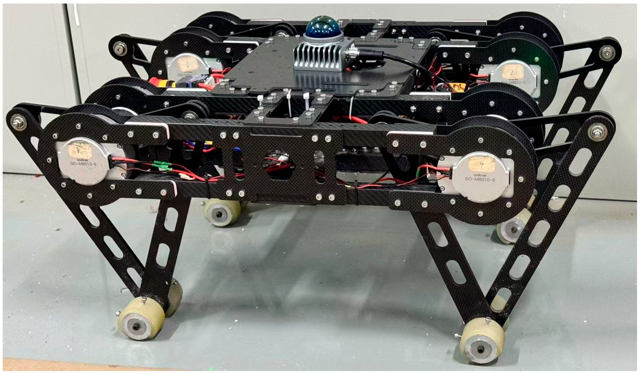
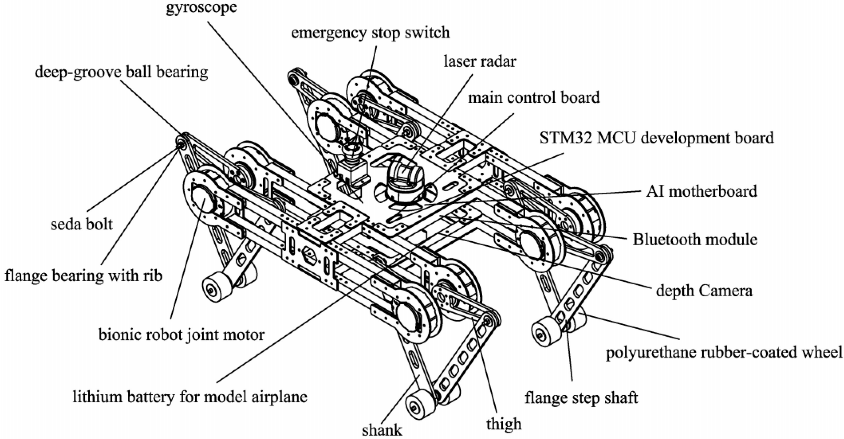
The mechanical structure of the quadruped robot was inspired by the physiological structure of mammals and consists of five parts. The legs are connected to the torso by four joints, with each joint having two degrees of freedom. Considering the balance between mechanical flexibility and complexity, the mechanical structure has been simplified. The simplified structure is shown in Figure 1 and consists of five parts. The parameters and structure of the four legs are identical and symmetrically distributed around the center. The kinematic model in its initial state is shown in Figure 2.

If the pose of the robot’s end-effector is given, the values of the other joints can be determined by performing inverse kinematics. There are two methods for solving inverse kinematics: The first is the analytical method, which is fast and accurate, utilizing algebraic calculation and geometric analysis for the solution. The second is the numerical method, which has a slower computation speed and unstable numerical iteration. Therefore, in this research, the geometric analysis approach from the analytical method was adopted to solve the inverse kinematics of the robot’s single leg.

The position inverse solution analysis involves determining the motor angles that achieve the desired foot-end trajectory, given the known lengths of the actuators AE and BC, as well as the lengths of the driven links ED and CD.

The continuous phase transition process of the foot-end of a single leg, from ground contact to liftoff, is referred to as the stance phase. The swing phase describes the continuous phase transition process in which the foot-end moves along the planned trajectory from liftoff to ground contact. During the stance phase, the leg supports the robot’s load and moves the torso in the target direction through phase transitions, shifting from the anterior extreme to the posterior extreme. Conversely, the swing phase shifts from the posterior extreme to the anterior extreme, determining the robot’s stride length and leg lift height when crossing obstacles. Therefore, research on the stance and swing phases is essential for deriving the torso trajectory of quadruped robots.

To study the stance phase of the right foreleg of the quadruped robot, we first assume that the parallel mechanism exhibits no lateral motion. The origin of the coordinate system is set at the center of the foot-end when the quadruped robot is in a static stance, with the forward direction aligned with the positive X-axis and the vertical direction upward along the positive Y-axis. The kinematic model under general conditions is shown in Figure 3.

From the geometric relationships and the law of cosines, we derive

$$c^2={(h_0-n)}^2+m^2$$

(1)

where $c$ represents the distance between the motor center and the foot-end center during movement, $h_0$ is the distance between the motor center and the foot-end center when stationary, $n$ is the horizontal distance of the foot-end, and $m$ is the vertical distance of the foot-end.

$$b^2=a^2+h_0^2-2a{h}_0\cos {\theta }_0$$

(2)

where $b$ is the length of the thigh, $a$ is the length of the calf, and ${\theta }_0$ is the angle between the stationary shin and the vertical axis.

$$\cos \gamma ={\displaystyle \frac{h_0-n}{c}}$$

(3)

where γ is the angle between the line connecting the motor center and the foot-end center and the vertical axis.

$$b^2=a^2+c^2-2ac\cos ({\theta }_1+{\theta }_0-\gamma )=a^2+c^2-2ac\cos ({\theta }_0+\gamma -{\theta }_2)$$

(4)

where ${\theta }_1$ is the angle between the moving thigh and the stationary thigh at the front, which represents the internal motor rotation, and ${\theta }_2$ is the angle between the moving thigh and the stationary thigh at the back, representing the external motor rotation.

From (3) and (4), the relationship between the two motor angles is derived as

$${\theta }_{1.}+{\theta }_2=2\gamma$$

(5)

$$\gamma =\arccos {\displaystyle \frac{h_0-n}{c}}$$

(6)

From (4) and (6), the expression for motor angle ${\theta }_1$ as a function of the foot-end position is

$${\theta }_1=\arccos {\displaystyle \frac{a^2+c^2-b^2}{2ac}}+\arccos {\displaystyle \frac{h_0-n}{c}}-{\theta }_0$$

(7)

From (5) and (7), the expression for motor angle ${\theta }_2$ as a function of the foot-end position is

$${\theta }_2=\arccos {\displaystyle \frac{h_0-n}{c}}-\arccos {\displaystyle \frac{a^2+c^2-b^2}{2ac}}+{\theta }_0$$

(8)

To investigate the stance phase of the quadruped robot’s right foreleg, it is assumed that the parallel mechanism does not undergo lateral motion. The foot-end center in the initial standing position during the stance phase is designated as the coordinate origin, with the forward direction aligned along the positive X-axis and the vertical direction upward along the positive Y-axis. The kinematic model under general conditions is illustrated in Figure 4.

Based on geometric relationships and the law of cosines, it can be derived as

$$b^2=a^2+l_0^2-2a{l}_0^2\cos {\beta }_0=a^2+d^2-2ad\cos {\beta }_1$$

(9)

where $l_0$ represents the initial distance between the motor and the foot-end, and ${\beta }_0$ is the angle between the thigh and the line connecting the motor and foot-end at the initial moment. $d$ represents the distance between the motor and the foot-end during motion, and ${\beta }_1$ is the corresponding angle during movement.

$$l_0^2=h_0^2+S^2$$

(10)

where $S$ denotes the step length.

$$d^2=x^2+y^2$$

(11)

where $x$ and $y$ represent the motor coordinates.

The relationship between the two motor angles is

$${\phi }_1={\phi }_2={\beta }_0-{\beta }_1$$

(12)

where ${\phi }_1$ denotes the inner motor angle and ${\phi }_2$ denotes the outer motor angle.

From Equations (9)–(12), the relationship between motor angles ${\phi }_1$ and ${\phi }_2$ and the motor position is given by

$${\phi }_1=\arccos {\displaystyle \frac{a^2-b^2+h_0^2+S^2}{2a{(h_0^2+S^2)}^{\frac{1}{2}}}}-\arccos {\displaystyle \frac{a^2-b^2+x^2+y^2}{2a{(x^2+y^2)}^{\frac{1}{2}}}}$$

(13)

The commonly used methods for the dynamics study of parallel robots include the Lagrange method, the Kane method, and the Newton-Euler method. In this section, the Lagrange method is used to establish the dynamic equation of the parallel leg mechanism, and the expression of the driving torque is obtained by solving the equation. The schematic diagram of the parallel leg mechanism is shown in Figure 5.

It is assumed that the position of the center of mass of each bar is on the common perpendicular of the adjacent joint axes. From the closed vector method and the projection relation, we can obtain

$$\left\{\begin{array}{c}a\cos {\theta }_6+b\cos {\theta }_5=a\cos {\theta }_4+b\cos {\theta }_3\\ a\sin {\theta }_6+b\sin {\theta }_5=a\sin {\theta }_4+b\sin {\theta }_3\end{array}\right.$$

(14)

where ${\theta }_3$ is the included angle between the left thigh and the positive direction of the X axis, ${\theta }_4$ is the included angle between the left crus and the positive direction of the X axis, ${\theta }_5$ is the included angle between the right thigh and the positive X axis direction, and ${\theta }_6$ is the included angle between the right crus and the positive X axis direction. The center of mass of each member is located on the common perpendicular of the adjacent joint axes. Choose ${\theta }_3$ and ${\theta }_5$ as generalized coordinates. It can be seen from Figure 3 and Figure 5 that

$$\left\{\begin{array}{l}{\theta }_3=270°-\left({\theta }_0+{\theta }_2\right)\\ {\theta }_6={\theta }_1+{\theta }_0-90°\end{array}\right.$$

(15)

It can be obtained from Formula (14) that

$$\left\{\begin{array}{l}{\theta }_4=2\arctan x_1\\ {\theta }_5=\arcsin \left({\displaystyle \frac{a\sin {\theta }_3-a\sin {\theta }_6-b\sin {\theta }_4}{b}}\right)\end{array}\right.$$

(16)

where $x_1={\displaystyle \frac{D\pm \sqrt{D^2-\left(A+B+C\right)\left(A+B-C\right)}}{A+B+C}}$, $A=2a^2$, $B=-2a^2\cos \left({\theta }_3-{\theta }_6\right)$, $C=2ab\left(\cos {\theta }_3-\cos {\theta }_6\right)$, and $D=2ab\left(\sin {\theta }_3-\sin {\theta }_6\right)$.

Take the partial derivative of Equation (14) with respect to ${\theta }_3$ and ${\theta }_6$, respectively, to obtain

$$\left\{\begin{array}{c}{\displaystyle \frac{\mathsf{\partial }{\theta }_5}{\mathsf{\partial }{\theta }_6}}=-{\displaystyle \frac{a\sin \left({\theta }_6-{\theta }_4\right)}{b\sin \left({\theta }_5-{\theta }_4\right)}}\\ {\displaystyle \frac{\mathsf{\partial }{\theta }_5}{\mathsf{\partial }{\theta }_3}}=-{\displaystyle \frac{a\sin \left({\theta }_4-{\theta }_3\right)}{b\sin \left({\theta }_5-{\theta }_4\right)}}\\ {\displaystyle \frac{\mathsf{\partial }{\theta }_4}{\mathsf{\partial }{\theta }_6}}=-{\displaystyle \frac{a\sin \left({\theta }_6-{\theta }_5\right)}{b\sin \left({\theta }_5-{\theta }_4\right)}}\\ {\displaystyle \frac{\mathsf{\partial }\theta 4}{\mathsf{\partial }{\theta }_3}}=-{\displaystyle \frac{a\sin \left({\theta }_5-{\theta }_3\right)}{b\sin \left({\theta }_5-{\theta }_4\right)}}\end{array}\right.$$

(17)

By taking the derivative of both sides of Equation (14), we can obtain

$$\left\{\begin{array}{c}a\cos {\theta }_6{\dot{\theta }}_6+b\cos {\theta }_5{\dot{\theta }}_5=b\cos {\theta }_3{\dot{\theta }}_3+a\cos {\theta }_4{\dot{\theta }}_4\\ a\sin {\theta }_6{\dot{\theta }}_6+b\sin {\theta }_5{\dot{\theta }}_5=b\sin {\theta }_3{\dot{\theta }}_3+a\sin {\theta }_4{\dot{\theta }}_4\end{array}\right.$$

(18)

Rewrite Equation (18) into a matrix form:

$$\left[\begin{array}{c}{\dot{\theta }}_5\\ {\dot{\theta }}_4\end{array}\right]=A\left[\begin{array}{c}{\dot{\theta }}_6\\ {\dot{\theta }}_3\end{array}\right]$$

(19)

where $A=G^{-1}H$, $G=\left[\begin{array}{cc}b\cos {\theta }_5& -b\cos {\theta }_4\\ b\sin {\theta }_5& -b\sin {\theta }_4\end{array}\right]$, and $H=\left[\begin{array}{cc}-a\cos {\theta }_1& a\cos {\theta }_4\\ -a\sin {\theta }_1& a\sin {\theta }_4\end{array}\right]$.

The position of the center of mass of each rod can be obtained from Figure 5 and the linear velocity of the center of mass of each rod can be obtained through time derivation.

The linear velocity of the center of mass of the right thigh center is

$$\left[\begin{array}{c}{\dot{x}}_{s4}\\ {\dot{y}}_{s4}\end{array}\right]=\left[\begin{array}{c}-q_1\sin {\theta }_6{\dot{\theta }}_6\\ -q_2\cos {\theta }_6{\dot{\theta }}_6\end{array}\right]$$

(20)

where ${\dot{x}}_{s4}$ is the horizontal linear velocity of the centroid of the right thigh and ${\dot{y}}_{s4}$ is the vertical linear velocity of the centroid of the right thigh. $q_1$ is the distance between the thigh mass center and the motor center and $q_2$ is the distance between the crus mass center and a joint connecting the thigh with the crus.

The linear velocity of the center of mass of the right lower leg is

$$\left[\begin{array}{c}{\dot{x}}_{s3}\\ {\dot{y}}_{s3}\end{array}\right]=\left[\begin{array}{c}-b\sin {\theta }_6{\dot{\theta }}_6-q_2\sin {\theta }_5{\dot{\theta }}_5\\ b\cos {\theta }_6{\dot{\theta }}_6+q_2\cos {\theta }_5{\dot{\theta }}_5\end{array}\right]$$

(21)

where ${\dot{x}}_{s3}$ is the linear velocity in the horizontal direction of the mass center of the right leg and ${\dot{y}}_{s3}$ is the linear velocity in the vertical direction of the mass center of the right leg.

The linear velocity of the center of mass of the left lower leg is

$$\left[\begin{array}{c}{\dot{x}}_{s2}\\ {\dot{y}}_{s2}\end{array}\right]=\left[\begin{array}{c}-a\sin {\theta }_3{\dot{\theta }}_3-q_2\sin {\theta }_4{\dot{\theta }}_4\\ a\cos {\theta }_3{\dot{\theta }}_3+q_2\cos {\theta }_4{\dot{\theta }}_4\end{array}\right]$$

(22)

where ${\dot{x}}_{s2}$ is the horizontal linear velocity of the mass center of the left leg and ${\dot{y}}_{s2}$ is the vertical linear velocity of the mass center of the left leg.

The linear velocity of the center of mass of the left thigh center is

$$\left[\begin{array}{c}{\dot{x}}_{s1}\\ {\dot{y}}_{s1}\end{array}\right]=\left[\begin{array}{c}-q_1\sin {\theta }_3{\dot{\theta }}_3\\ q_1\cos {\theta }_3{\dot{\theta }}_3\end{array}\right]$$

(23)

where ${\dot{x}}_{s1}$ is the horizontal linear velocity of the mass center of the left thigh and ${\dot{y}}_{s1}$ is the vertical linear velocity of the mass center of the left thigh.

According to (16) and (19)–(23), the total kinetic energy of the system is expressed as

$$\begin{array}{cc}\hfill E& ={\displaystyle \sum _{i=1}^4\frac{1}{2}}\left[m_i\left({\dot{x}}_{si}^2+{\dot{y}}_{si}^2\right)+J_i{\dot{\theta }}_{i+2}^2\right]\hfill \\ & ={\displaystyle \frac{1}{2}}\left[\left(m_1{\dot{x}}_{s1}^2+m_1{\dot{y}}_{s1}^2+m_2{\dot{x}}_{s2}^2+m_2{\dot{y}}_{s2}^2+m_3{\dot{x}}_{s3}^2+m_3{\dot{y}}_{s3}^2+m_4{\dot{x}}_{s4}^2+m_4{\dot{y}}_{s4}^2\right)\right.\hfill \\ & +\left.\left(J_1{\dot{\theta }}_3^2+J_2{\dot{\theta }}_4^2+J_3{\dot{\theta }}_5^2+J_4{\dot{\theta }}_6^2\right)\right]\hfill \\ & ={\displaystyle \frac{1}{2}}{J}_{33}{\dot{\theta }}_3^2+J_{36}{\dot{\theta }}_3{\dot{\theta }}_6+{\displaystyle \frac{1}{2}}{J}_{66}{\dot{\theta }}_6^2\hfill \end{array}$$

(24)

where the masses of the left thigh, left calf, right calf, and right thigh are $m_1$, $m_2$, $m_3$, and $m_4$, respectively, and the moments of inertia of the left thigh, left calf, right calf, and right thigh around the center of mass are $J_1$, $J_2$, $J_3$, and $J_4$, respectively, and $m_1=m_4$, $m_2=m_3$, $J_1=J_4$, and $J_2=J_3$. The coefficients $J_{33}$, $J_{66}$, and $J_{36}$ are, respectively, expressed as

$$J_{33}=J_1+m_1{q}_1^2+m_2\left[a^2+2a{q}_2{\displaystyle \frac{\mathsf{\partial }{\theta }_4}{\mathsf{\partial }{\theta }_3}}\cos \left({\theta }_4-{\theta }_3\right)\right]+\left(m_3{q}_2^2+J_3\right){\left({\displaystyle \frac{\mathsf{\partial }{\theta }_5}{\mathsf{\partial }{\theta }_3}}\right)}^2+\left(m_2{q}_2^2+J_2\right){\left({\displaystyle \frac{\mathsf{\partial }{\theta }_4}{\mathsf{\partial }{\theta }_3}}\right)}^2$$

(25)

$$J_{66}=J_4+m_4{q}_1^2+m_3\left[a^2+2a{q}_2{\displaystyle \frac{\mathsf{\partial }{\theta }_5}{\mathsf{\partial }{\theta }_6}}\cos \left({\theta }_5-{\theta }_6\right)\right]+\left(m_3{q}_2^2+J_3\right){\left({\displaystyle \frac{\mathsf{\partial }{\theta }_5}{\mathsf{\partial }{\theta }_6}}\right)}^2+\left(m_2{q}_2^2+J_2\right){\left({\displaystyle \frac{\mathsf{\partial }{\theta }_4}{\mathsf{\partial }{\theta }_6}}\right)}^2$$

(26)

$$\begin{array}{rr}{J}_{36}& =\left(m_3{q}_2^2+J_3\right)\left({\displaystyle \frac{\mathsf{\partial }{\theta }_5}{\mathsf{\partial }{\theta }_3}}·{\displaystyle \frac{\mathsf{\partial }{\theta }_5}{\mathsf{\partial }{\theta }_6}}\right)+\left(m_2{q}_2^2+J_2\right)\left({\displaystyle \frac{\mathsf{\partial }{\theta }_4}{\mathsf{\partial }{\theta }_3}}·{\displaystyle \frac{\mathsf{\partial }{\theta }_4}{\mathsf{\partial }{\theta }_6}}\right)\hfill \\ & +m_{3}a{q}_2{\displaystyle \frac{\mathsf{\partial }{\theta }_5}{\mathsf{\partial }{\theta }_3}}\cos \left({\theta }_5-{\theta }_6\right)+m_{2}a{q}_2{\displaystyle \frac{\mathsf{\partial }{\theta }_4}{\mathsf{\partial }{\theta }_6}}\cos \left({\theta }_4-{\theta }_3\right)\hfill \end{array}$$

(27)

The total potential energy of the legs can be expressed as

$$U={\displaystyle \sum _i^4{m}_i}g{h}_1$$

(28)

where the height of the center of mass of the left thigh, the left leg, the right leg, and the right thigh from the ground is $h_1$, $h_2$, $h_3$, and $h_4$, respectively.

The driving moments $M_1$ and $M_2$ can be obtained from the Lagrangian equation $M_I={\displaystyle \frac{d}{dt}}\left({\displaystyle \frac{\mathsf{\partial }E}{\mathsf{\partial }{\dot{\theta }}_{i+2}}}\right)-{\displaystyle \frac{\mathsf{\partial }E}{\mathsf{\partial }{\theta }_{i+2}}}+{\displaystyle \frac{\mathsf{\partial }U}{\mathsf{\partial }{\dot{\theta }}_{i+2}}}$ as follows:

$$\left\{\begin{array}{c}{M}_1=J_{66}{\ddot{\theta }}_6+J_{36}{\ddot{\theta }}_3+{\displaystyle \frac{1}{2}}{\displaystyle \frac{\mathsf{\partial }{J}_{66}}{\mathsf{\partial }{\theta }_6}}{\dot{\theta }}_6^2+\left({\displaystyle \frac{\mathsf{\partial }{J}_{36}}{\mathsf{\partial }{\theta }_3}}-{\displaystyle \frac{1}{2}}{\displaystyle \frac{\mathsf{\partial }{J}_{33}}{\mathsf{\partial }{\theta }_6}}\right){\dot{\theta }}_3^2+{\displaystyle \frac{\mathsf{\partial }{J}_{66}}{\mathsf{\partial }{\theta }_3}}{\dot{\theta }}_3{\dot{\theta }}_6\\ M_2=J_{33}{\ddot{\theta }}_3+J_{36}{\ddot{\theta }}_6+{\displaystyle \frac{1}{2}}{\displaystyle \frac{\mathsf{\partial }{J}_{33}}{\mathsf{\partial }{\theta }_3}}{\dot{\theta }}_3^2+\left({\displaystyle \frac{\mathsf{\partial }{J}_{36}}{\mathsf{\partial }{\theta }_6}}-{\displaystyle \frac{1}{2}}{\displaystyle \frac{\mathsf{\partial }{J}_{66}}{\mathsf{\partial }{\theta }_3}}\right){\dot{\theta }}_6^2+{\displaystyle \frac{\mathsf{\partial }{J}_{33}}{\mathsf{\partial }{\theta }_6}}{\dot{\theta }}_3{\dot{\theta }}_6\end{array}\right.$$

(29)

In the gait cycle of a quadruped walking robot, the torso movement follows a regular pattern. Therefore, it is necessary to deduce the robot’s torso trajectory from the foot-end trajectory, specifically calculating the actual trajectory of the foot during single-leg movement.

To enhance the adaptability of quadruped robots to unstructured environments and ability to efficiently complete assigned tasks, the trot gait is generally used as the ideal state. In the trot gait, the duty cycle is 0.5, meaning that the robot’s diagonal legs move in sync, both either in the swing phase or in the stance phase.

The foot-end trajectory of the quadruped robot adopts the earliest composite cycloid trajectory. The stance phase and swing phase each occupy half of the total cycle. When the foot-end is in the swing phase, the trajectory equation of the quadruped robot’s foot-end relative to the torso is given by the following equation:

$$\left\{\begin{array}{l}m=S\left[0.5-{\displaystyle \frac{1}{2\pi }}\sin \left({\displaystyle \frac{2\pi t}{T}}\right)\right]\\ n=H\left[0.5-0.5\cos \left({\displaystyle \frac{2\pi t}{T}}\right)\right]\end{array}\right.$$

(30)

where $H$ represents the lift height, $T$ is the cycle, and $t$ is the time.

The foot-end trajectory during the swing phase of the quadruped robot is corrected. Since the quadruped robot uses the trot gait, the foot-end trajectory should be the vector sum of the torso trajectory, which is derived from the inverse of the composite cycloid trajectory planned during the stance phase and the theoretical sine trajectory planned during the swing phase. The absolute trajectory equation of the foot-end during the swing phase is thus given by

$$\left\{\begin{array}{l}m=2S\left[0.5-{\displaystyle \frac{1}{2\pi }}\sin \left({\displaystyle \frac{2\pi t}{T}}\right)\right]\\ n=2H\left[0.5-0.5\cos \left({\displaystyle \frac{2\pi t}{T}}\right)\right]\end{array}\right.$$

(31)

Since the stance phase moves the robot’s torso by changing the leg phase to achieve movement in the target direction, the motor rotation pattern can be derived through the analysis of the stance phase. By taking the first derivative of (13) with respect to time, the expression for the motor’s angular velocity can be obtained:

$$\dot{\phi }={\displaystyle \frac{(\dot{x}x+\dot{y}y)(a^2-b^2-x^2-y^2)}{(x^2+y^2)\sqrt{4a^2(x^2+y^2)-{(a^2-b^2+x^2+y^2)}^2}}}$$

(32)

By taking the second derivative of (13) with respect to time, the angular acceleration expression for motor rotation is obtained:

$$\ddot{\phi }={\displaystyle \frac{\left(\sigma -\mu \right)\left[2{\lambda }^2\left[\delta +\mu (a^2+b^2-\mu )\right]-\mu \delta \left(\ddot{x}x+\ddot{y}y+{\dot{x}}^2+{\dot{y}}^2\right)\right]-2{\lambda }^2\mu \delta }{\mu {\delta }^{\frac{3}{2}}}}$$

(33)

where $\lambda =\dot{x}x+\dot{y}y$, $\mu =x^2+y^2$, $\sigma =a^2+b^2$, and $\delta =4a^2\mu -{\left(\sigma +\mu \right)}^2$.

Since the quadruped robot uses the trot gait with a duty cycle of 0.5, and the foot trajectory is planned using a composite cycloid curve, kinematic analysis reveals that the trajectory equations of the robot’s torso match those of the foot relative to the driving mechanism:

$$\left\{\begin{array}{l}x=S\left[{\displaystyle \frac{t}{T}}-{\displaystyle \frac{1}{2\pi }}\sin \left({\displaystyle \frac{2\pi t}{T}}\right)\right]\\ y=H\left[0.5-0.5\cos \left({\displaystyle \frac{2\pi t}{T}}\right)\right]\end{array}\right.$$

(34)

$$\dot{x}={\displaystyle \frac{S}{T}}-{\displaystyle \frac{S}{T}}\cos \left({\displaystyle \frac{2\pi t}{T}}\right)$$

(35)

$$\ddot{x}={\displaystyle \frac{2\pi S}{T^2}}\sin \left({\displaystyle \frac{2\pi t}{T}}\right)$$

(36)

Using the state variables ${\left[x,\dot{x}\right]}^T$ from (34)–(36), we obtain

$$\left(\begin{array}{l}\ddot{x}\\ \dot{x}\end{array}\right)=\left(\begin{array}{cc}0& -{\displaystyle \frac{4{\pi }^2}{T^2}}\\ 1& 0\end{array}\right)\left(\begin{array}{l}\dot{x}\\ x\end{array}\right)+\left(\begin{array}{c}{\displaystyle \frac{4{\pi }^{2}St}{T^3}}\\ 0\end{array}\right)$$

(37)

Through a forward kinematics analysis of the swing phase, setting $b=2a$ and ${\theta }_0=121.83°$, the following geometric relationship is derived:

$$\begin{array}{cc}m& =\left[a\cos \left({\theta }_0+{\displaystyle \frac{{\theta }_1-{\theta }_2}{2}}\right)+\sqrt{b^2-a^2{\sin }^2\left({\theta }_0+{\displaystyle \frac{{\theta }_1-{\theta }_2}{2}}\right)}\right]\sin {\displaystyle \frac{{\theta }_1+{\theta }_2}{2}}\hfill \\ & =a\left(\cos {\theta }_0\right)\sin {\displaystyle \frac{{\theta }_1+{\theta }_2}{2}}+\sin {\displaystyle \frac{{\theta }_1+{\theta }_2}{2}}\sqrt{b^2-a^2{\sin }^2\left({\theta }_0\right)}\hfill \\ & =-0.5a\sin {\displaystyle \frac{{\theta }_1+{\theta }_2}{2}}+\sin {\displaystyle \frac{{\theta }_1+{\theta }_2}{2}}\sqrt{b^2-0.75a^2}\hfill \\ & =1.3a\sin {\displaystyle \frac{{\theta }_1+{\theta }_2}{2}}\hfill \end{array}$$

(38)

Next, we analyzed the stance phase. From [32], the motor state equations can be described as

$$\left\{\begin{array}{l}{\dot{z}}_1=z_2\\ {\dot{z}}_2={\displaystyle \frac{1}{J_0}}\left(K_{1}u-K_2{z}_2+T^{\ast }\right)\end{array}\right.$$

(39)

The state variables $z={\left[z_1,z_2\right]}^T$ represent the motor’s position and angular velocity, $J_0$ is the inertia, and $T^{\ast }$ denotes the torque vector.

For the quadruped robot’s joint motors, let $q={\left[q_1,q_2\right]}^T$, $q_2={\theta }_1$, and $q_2={\dot{\theta }}_1$, leading to

$$\left\{\begin{array}{l}{\dot{q}}_1=q_2\\ {\dot{q}}_2={\displaystyle \frac{1}{J_0}}\left(K_{1}u-K_2{q}_2+T^{\ast }\right)\end{array}\right.$$

(40)

Therefore, (40) can be expressed as

$$\dot{q}=\eta \left(q\right)+\nu \left(q\right)u$$

(41)

where $\nu \left(q\right)={\left(0,{\displaystyle \frac{K_1}{J_0}}\right)}^T$.

Let $\eta \left(q\right)={\left[q_2,{\displaystyle \frac{1}{J_0}}\left(-K_2{q}_2+T^{\ast }\right)\right]}^T$, and the state variables of the quadruped robot are $X={\left[X_1,X_2\right]}^T$, where $X_1$ represents displacement and $X_2$ represents velocity. Let ${\theta }_2=2\gamma -{\theta }_1$ be denoted as $h\left({\theta }_1\right)$. Based on (37) and (39), the overall system equations of the quadruped robot can be expressed as

$${\dot{X}}_1=X_2={\displaystyle \frac{13a^2\left(q_1+q_1\dot{h}\left({\theta }_1\right)\right)}{20}}{\mathrm{c}}_{11}-{\displaystyle \frac{\left(q_1-q_1\dot{h}\left({\theta }_1\right)\right)}{40}}\left[17a+{\displaystyle \frac{a}{5}}{s}_{11}\right]$$

(42)

$$\begin{array}{cc}{\dot{X}}_2& ={\displaystyle \frac{13a^2}{20}}\left({\dot{q}}_1+{\dot{q}}_1\dot{h}\left({\theta }_1\right)+q_1^2\ddot{h}\left({\theta }_1\right)\right)c_{11}-{\displaystyle \frac{13{\left(q_1+q_1\dot{h}\left({\theta }_1\right)\right)}^2}{40}}{s}_{11}\hfill \\ & -{\displaystyle \frac{\left({\dot{q}}_1-{\dot{q}}_1\dot{h}\left({\theta }_1\right)-q_1^2\ddot{h}\left({\theta }_1\right)\right)a}{40}}\left[17+0.2s_{11}\right]-{\displaystyle \frac{a{q}_1^2\left(1-\dot{h}{\left({\theta }_1\right)}^2\right)}{400}}{c}_{11}\hfill \end{array}$$

(43)

where $s_{11}=\sin \left({\displaystyle \frac{{\theta }_1+h\left({\theta }_1\right)}{2}}\right)$ and $c_{11}=\cos \left({\displaystyle \frac{{\theta }_1+h\left({\theta }_1\right)}{2}}\right)$.

By defining

$$\begin{array}{cc}\dot{X}& =\dot{h}\left(q\right)\hfill \\ & =\nabla h\left(q\right)\left(f_0\left(q\right)+g_0\left(q\right)u\right)\hfill \\ & \triangleq f\left(X\right)+g\left(X\right)u\hfill \end{array}$$

(44)

Let the tracking parameter $X_d={\left[X_{1d},X_{2d}\right]}^T$. Similarly to [33], we constructed an augmented system:

$$\begin{array}{cc}\dot{X}& =\left[\begin{array}{c}f\left(X\right)-X_d\\ {\dot{X}}_d\end{array}\right]+\left[\begin{array}{c}g\left(X\right)\\ 0\end{array}\right]u\hfill \\ & \triangleq F\left(X\right)+G\left(X\right)u\hfill \end{array}$$

(45)

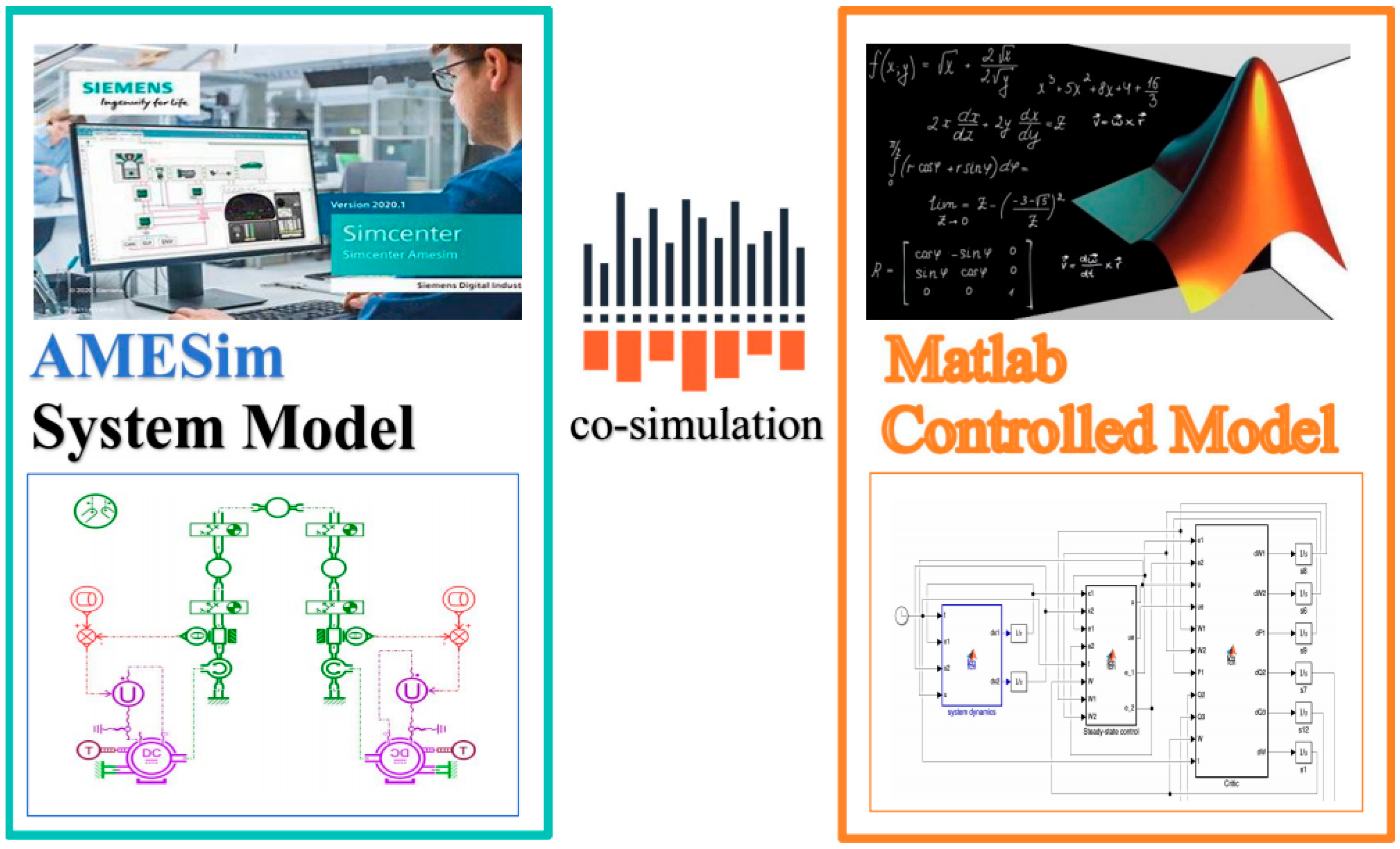
Remark 1.

Due to the nonlinearity of the system, especially in the dynamics of robotic joint torque, direct linearization may lose some dynamic characteristics. However, it is difficult to obtain specific expressions of $f\left(X\right)$ and $g\left(X\right)$ without further simplification. In this paper, we opted to use AMESim and Simulink for co-simulation instead of manually building complex state equation models. AMESim accurately simulates the dynamic behavior, motion variations, and interaction characteristics of the multi-robot system, eliminating the need to manually construct detailed kinematic and mechanical coupling equations. This approach significantly simplifies the modeling process and enhances the accuracy of the simulation results. Simulink was employed to implement the control algorithm, and the proposed algorithm is model-free. This process will be explained in detail in Section 4.

3. Optimal Controller Design

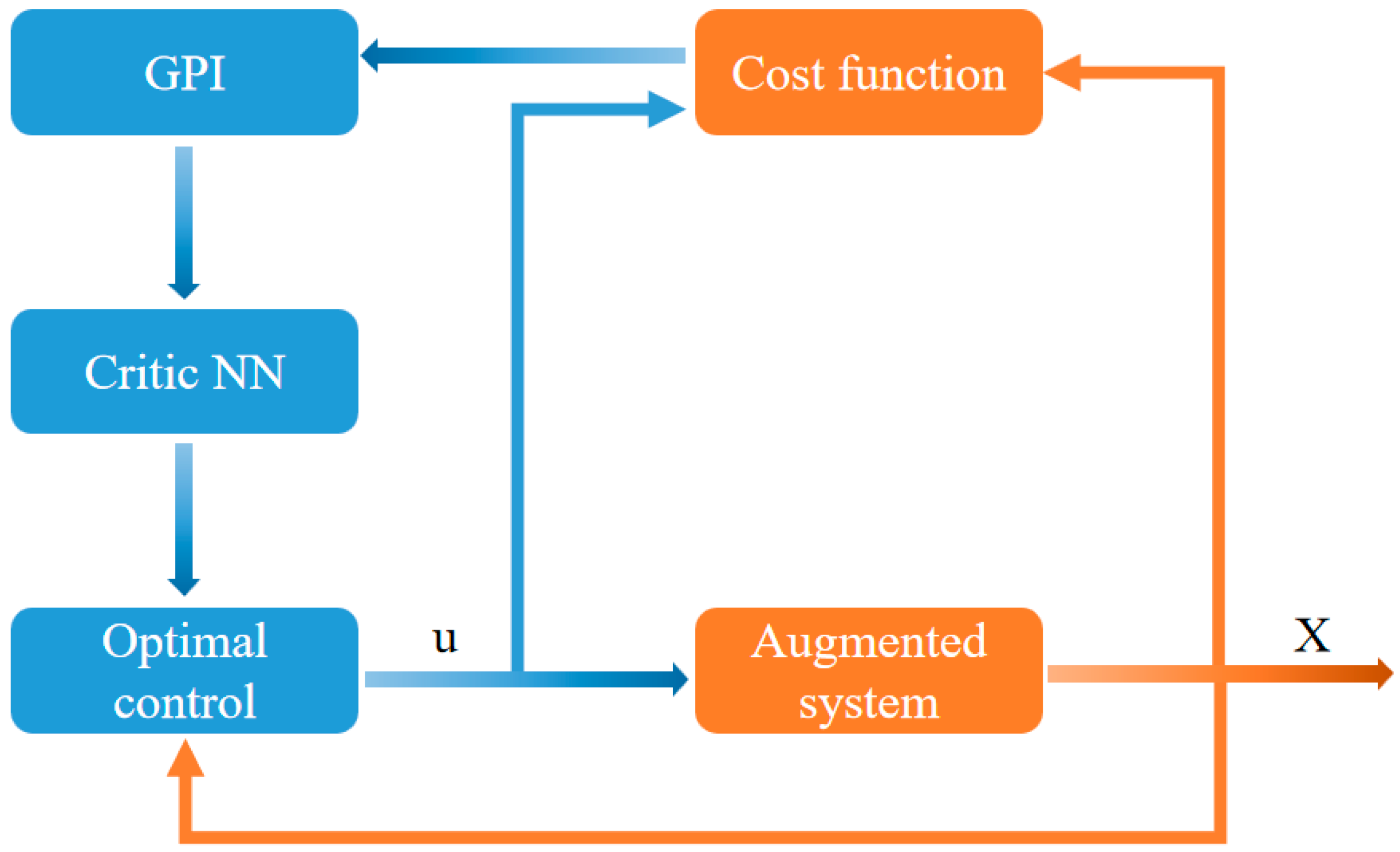
This section presents the general formula for the infinite horizon nonlinear optimal control problem in continuous time systems. The flow chart of the algorithm in this paper can be seen in Figure 6.

In Section 2, we defined the control system for the quadruped robot as follows:

$$\dot{X}\left(t\right)=F\left(X\right)+G\left(X\right)u,X\left(0\right)=X_0$$

(46)

where $X\left(t\right)\in {ℝ}^n$ represents the state vector, $u\left(t\right)\in {ℝ}^m$ is the control input or strategy, and $F\left(X\left(t\right)\right)\in {ℝ}^n$ and $G\left(X\right)\in {ℝ}^{n\times m}$ are the system and input gain functions, respectively. The value function $V\left(X\right)$ is defined as the infinite horizon cost:

$$V\left(X\right)={\displaystyle {\int }_t^{\infty }r\left(S\left(X\left(\tau \right)\right),u\left(\tau \right)\right)}d\tau$$

(47)

where $r=S\left(X\left(t\right)\right)+u^T\left(t\right)Ru\left(t\right)$ with $R$ is a positive definite matrix, and $S\left(X\left(t\right)\right)\in ℝ$.

Assumption 1.

Assume that $F\left(X\right)+G\left(X\right)u$ satisfies Lipschitz continuity on a compact set $\Theta \in {ℝ}^n$ that contains the origin, and the system (46) is stable, meaning that the state $X$ converges to a stable control law $u$.

The optimal control problem is solved by selecting the optimal stabilizing control $u^{\ast }\left(t\right)$ that minimizes the value function in (47). The optimal value function $V^{\ast }\left(X\right)$ is defined as

$$V^{\ast }\left(X\left(t\right)\right)=\underset{u}{\min }{\displaystyle {\int }_t^{\infty }r\left(X\left(\tau \right)\right),u\left(\tau \right)}d\tau$$

(48)

The partial differential equation of the optimal value function $V^{\ast }\left(X\right)$ can be expressed as a general solution to the nonlinear optimal control problem. We define the Hamiltonian for this problem as

$$\Psi \left(X,u,\nabla V_X\right)=r\left(X,u\right)+{\left(\nabla V_X\right)}^T\left(F\left(X\right)+G\left(X\right)u\right)$$

(49)

where the gradient vector is $\nabla V_X=\mathsf{\partial }V/\mathsf{\partial }X\in {ℝ}^n$. The optimal value function $V^{\ast }\left(X\right)$ from (48) satisfies the Hamilton–Jacobi–Bellman (HJB) equation:

$$0=\underset{u}{\min }\Psi \left(X,u,\nabla V_X^{\ast }\right)$$

(50)

For the unconstrained control $u$, the optimal control $u^{\ast }$ can be found by setting $\mathsf{\partial }\Psi \left(X,u,\nabla V_X^{\ast }\right)/\mathsf{\partial }u=0$, hence

$$u^{\ast }=-{\displaystyle \frac{1}{2}}{R}^{-1}F{\left(X\right)}^T\nabla V_X^{\ast }$$

(51)

Substituting the optimal control expression (51) into (50) yields the HJB equation based on $\nabla V_X^{\ast }$:

$$0=S\left(x\right)+{\left(\nabla V_X^{\ast }\right)}^{T}F\left(X\right)-{\displaystyle \frac{1}{4}}{\left(\nabla V_X^{\ast }\right)}^{T}G\left(X\right)R^{-1}G{\left(X\right)}^T\nabla V_X^{\ast }$$

(52)

Given the nonlinearity of the HJB (50) and the requirement for an accurate understanding of the system dynamics $F\left(X\right)$ and the input gain $G\left(X\right)$, solving the equation is typically challenging.

Remark 2.

Policy iteration is a reinforcement learning method used to determine optimal values and control strategies. By alternating between policy evaluation and policy improvement, it incrementally converges towards the optimal policy. This approach has led to the development of various algorithms, as described in [34,35], which are designed to solve the HJB equation either in real time or in advance. In the discussion within this section, policy evaluation and improvement occur synchronously, as both the critic and actor are updated simultaneously. This process is considered an extreme form of Generalized Policy Iteration (GPI).

In continuous time systems, policy evaluation can be achieved using adaptive critics, with the core involving the solution of a nonlinear Lyapunov equation (e.g., [35,36]). The derivation of such equations can be via Leibniz’s formula for differentiating the value function [35]. Additionally, another approach for solving the Bellman equation is through Integral Reinforcement Learning (IRL) [37].

$$V\left(X\left(t-T\right)\right)={\displaystyle {\int }_{t-T}^{t}r\left(X\left(\tau \right),u\left(\tau \right)\right)d\tau +V\left(X\left(t\right)\right)}$$

(53)

Let the period $T>0$. This is a discrete time Bellman equation, similar to the integral form. Note that the system equation $F\left(X\right)$ and input gain $G\left(X\right)$ in the Lyapunov equation do not appear in the Bellman (53). For policy improvement, following [38], the control is iteratively obtained by solving the value function $V$ (53), as follows:

$$u=-{\displaystyle \frac{1}{2}}{R}^{-1}G{\left(X\right)}^T\nabla V_X$$

(54)

The system will converge to the optimal control $u^{\ast }$ from (51).

3.1. Value Function Approximation with Adaptive Critic

This section introduces a novel design for policy evaluation using an adaptive critic. We approximate the value function through a critic neural network:

$$V\left(X\right)=w^T\varphi \left(X\right)+\xi \left(X\right)$$

(55)

where $\varphi \left(X\right):{ℝ}^n\to {ℝ}^N$ in the activation vector with $N$ hidden neurons, and $w\in {ℝ}^N$ is the weight vector. $\xi \left(X\right)\in ℝ$ represents the approximation error of the neural network. By selecting appropriate activation functions, a complete set of independent bases can be constructed to ensure the accurate approximation of $V\left(X\right)$. According to the Weierstrass higher order approximation theorem [38], within a compact set $\Theta$, as the number of neurons $N\to \infty$, for a fixed $N$, the approximation error $\xi \left(X\right)$ and its gradient $\nabla {\xi }_X$ approach zero, i.e., $\xi \left(X\right)\to 0$ and $\nabla {\xi }_X\to 0$.

We applied the Bellman method to update the critic. Substituting the approximated value function (55) into the Bellman equation (53) gives

$$\underset{R\left(X,u\right)}{\underbrace{{\displaystyle {\int }_{t-T}^{t}r\left(X\left(\tau \right),u\left(\tau \right)\right)d\tau }}}+\underset{w^T\Delta \varphi \left(t\right)}{\underbrace{w^T\varphi \left(X\left(t\right)\right)-w^T\varphi \left(X\left(t-T\right)\right)}}=-{\xi }_B$$

(56)

By using integral reinforcement $R\left(X,u\right)$, the difference $\Delta \varphi \left(t\right)=\varphi \left(X\left(t\right)\right)-\varphi \left(X\left(t-T\right)\right)$, and the Bellman equation, the residual error ${\xi }_B=\xi \left(X\left(t\right)\right)-\xi \left(X\left(t-T\right)\right)$ is bounded within the compact set $\Theta$, ensuring that $\xi \left(X\right)$ remains within bounds. To design an adaptive law for the weight vector that guarantees the convergence of the value function approximation, we introduce the auxiliary variables $M_1\in {ℝ}^{N\times N}$ and $N_1\in {ℝ}^N$ through the low-pass-filtered variables in (56):

$$\left\{\begin{array}{c}{\dot{M}}_1=-\mathcal{l}{M}_1+\Delta \varphi \left(t\right)\Delta \varphi {\left(t\right)}^T,M_1\left(0\right)=0\\ {\dot{N}}_1=-\mathcal{l}{N}_1+\Delta \varphi \left(t\right)R\left(X,u\right),N_1\left(0\right)=0\end{array}\right.$$

(57)

Here, the filtering parameter $\mathcal{l}>0$ and the discount factor $\mathcal{l}$ are introduced to ensure exponential decay, effectively preventing unbounded growth in the values of $M_1\left(t\right)$ and $N_1\left(t\right)$ while maintaining stability. $M_1$ and $N_1$ are defined as follows:

$$\left\{\begin{array}{l}{M}_1\left(t\right)={\displaystyle {\int }_0^t{e}^{-\mathcal{l}\left(t-\tau \right)}\Delta \varphi \left(\tau \right)\Delta {\varphi }^T\left(\tau \right)}d\tau \\ N_1\left(t\right)={\displaystyle {\int }_0^t{e}^{-\mathcal{l}\left(t-\tau \right)}\Delta \varphi \left(\tau \right)R\left(\tau \right)}d\tau \end{array}\right.$$

(58)

Definition 1.

(Persistency of excitation (PE) [39]). If there exists a strictly positive constant ${\sigma }_1>0$ such that the following condition holds over the interval $\Delta \phi \left(t\right)$, the signal $\left[t-T,t\right]$ is said to be persistently excited, i.e.,

$${\displaystyle {\int }_{t-T}^t\Delta \varphi \left(\tau \right)}\Delta \varphi {\left(\tau \right)}^{T}d\tau \ge {\sigma }_{1}I,\forall t>0$$

(59)

The PE condition [39] is widely required in adaptive control to ensure parameter convergence.

Lemma 1.

([40]). If the signal $\Delta \phi \left(t\right)$ is persistently excited for all $t>0$, then the auxiliary variable $M_1$ defined in (57) is positive definite, i.e., $M_1>0$, and the minimum eigenvalue ${\lambda }_{\min }\left(M_1\right)>{\sigma }_1>0$, $\forall t>0$.

Proof. 

Detailed proof can be found in [40].

The adaptive critic neural network can be expressed as

$$\widehat{V}\left(X\right)={\widehat{w}}^T\varphi \left(X\right)$$

(60)

where $\widehat{w}$ and $\widehat{V}\left(X\right)$ represent the current estimates of $w$ and $V\left(X\right)$, respectively. We now design an adaptive law to update $\widehat{w}$ using a sliding mode technique, defined as follows:

$$\dot{\widehat{w}}=-{\Gamma }_1{M}_1{\displaystyle \frac{P_1}{‖P_1‖}}$$

(61)

$P_1\in {ℝ}^N$ is defined as $P_1=M_1\widehat{w}+N_1$, and ${\Gamma }_1>0$ is a positive adjustment gain to be determined in [36]. This gain facilitates the adaptive learning process. □

Lemma 2.

Considering the adaptive law (61), if the system state $X\left(t\right)$ remains bounded under a given stable control, and if $u\left(t\right)$, $\varphi \left(t\right)$ , and the system state $X\left(t\right)$ are persistently excited, then the estimation error $\tilde{w}=w-\widehat{w}$ satisfies the following conditions:

If the approximation error of the neural network $\xi \left(X\right)$ is zero, the estimation error $\widehat{w}$ will converge to zero within a finite time $t_1>0$.

If $\xi \left(X\right)\ne 0$, the estimation error $\widehat{w}$ will converge to a compact set within a finite time $t_1>0$.

Proof. 

We begin by examining the boundedness of $P_1$. In Equation (58), when the states $X\left(t\right)$ and $X\left(t-T\right)$ are bounded, the matrix $M_1$ is positive and has an upper bound ${\delta }_{M_1}>0$ , such that ${\lambda }_{\max }\left(M_1\right)\le {\delta }_{M_1}$. Due to the Bellman equation, the residual error ${\xi }_B$ is bounded. By introducing some constants ${\delta }_1>0$ and substituting $R$ into Equations (56)–(58), we find that $Q_1=-M_{1}w+{\Lambda }_1$ is also bounded, where ${\Lambda }_1$ is given by ${\Lambda }_1=\left(t\right)={\displaystyle {\int }_0^t{e}^{-\mathcal{l}\left(t-\tau \right)}\Delta \phi \left(\tau \right){\xi }_B}\left(\tau \right)d\tau$ . Thus, $M_1$ can be expressed as

$$P_1=-M_1\tilde{w}+{\Lambda }_1$$

(62)

Since $\Delta \phi \left(t\right)$ is persistently excited, from Lemma 1, we know that $M_1$ is symmetric and positive definite, and thus invertible. Therefore, we have $M_1^{-1}{P}_1=-\tilde{w}+M_1^{-1}{\Lambda }_1$. Here, $M_1^{-1}{P}_1$ can be used to design a suitable Lyapunov function, as it includes both the estimation error $\tilde{w}$ and ${\Lambda }_1$. We differentiate $M_1^{-1}{P}_1$ as follows:

$${\displaystyle \frac{\mathsf{\partial }}{\mathsf{\partial }t}}\left(M_1^{-1}{P}_1\right)=-\dot{\tilde{w}}+{\displaystyle \frac{\mathsf{\partial }{M}_1^{-1}}{\mathsf{\partial }t}}{\Lambda }_1+M_1^{-1}{\dot{\Lambda }}_1=\dot{\widehat{w}}+{\overline{\Lambda }}_1$$

(63)

where ${\overline{\Lambda }}_1=-M_1^{-1}{\dot{M}}_1{M}_1^{-1}{\Lambda }_1+M_1^{-1}{\dot{\Lambda }}_1$ and ${\Lambda }_1$ is bounded, meaning that $‖{\overline{\Lambda }}_1‖\le {\overline{\delta }}_1$ for some constants ${\overline{\delta }}_1>0$. Note that $M_1^{-1}$ is bounded since ${\lambda }_{\min }\left(M_1\right)>{\sigma }_1$ and ${\lambda }_{\max }\left(M_1\right)<{\delta }_{M_1}$. Therefore, the upper and lower bounds for $M_1^{-1}$ can easily be derived as ${\lambda }_{\min }\left(M_1^{-1}\right)>{\delta }_{M_1}$ and ${\lambda }_{\max }\left(M_1^{-1}\right)<1/{\sigma }_1$. Consequently, we can easily find the lower and upper bounds for the two $\Psi$-type functions in $P_1$ [41], which serve as the lower and upper bounds of the following modified Lyapunov function:

$${\Psi }_1={\displaystyle \frac{L_1}{2}}{\left(M_1^{-1}{P}_1\right)}^T{\Gamma }_1^{-1}{M}_1^{-1}{P}_1$$

(64)

where $L_1>0$ is a constant. The time derivative can be calculated as

$$\begin{array}{cc}{\dot{\Psi }}_1& =L_1{P}_1^T{M}_1^{-1}{\Gamma }_1^{-1}\left(\dot{\widehat{w}}+{\overline{\Lambda }}_1\right)\hfill \\ & =L_1{P}_1^T{M}_1^{-1}{\Gamma }_1^{-1}\left(-{\Gamma }_1^{-1}{M}_1{\displaystyle \frac{P_1}{‖P_1‖}}+{\overline{\Lambda }}_1\right)\hfill \\ & \le -{\alpha }_1\sqrt{{\Psi }_1}\hfill \end{array}$$

(65)

where ${\alpha }_1=\left({\sigma }_1-L_1{\overline{\delta }}_1{\lambda }_{\max }\left({\Gamma }_1^{-1}\right)\right)\sqrt{2/{\lambda }_{\max }\left({\Gamma }_1^{-1}\right)}$ is a positive constant for a properly chosen $L_1$ with $0<L_1<{\sigma }_1/{\lambda }_{\max }\left({\Gamma }_1^{-1}\right){\overline{\delta }}_1$. Based on [42], we can conclude that ${\Psi }_1=0$ and $P_1=0$ within a finite time $t_1=2\sqrt{{\Psi }_1\left(0\right)}/{\alpha }_1>0$. Thus, we have the following results:

• In the case where $\xi \left(X\right)=0$, we find that ${\xi }_B=0$, $P_1=0$, and ${\Lambda }_1={\overline{\Lambda }}_1=0$, meaning that $\tilde{w}=0$ with ${\alpha }_1={\sigma }_1\sqrt{2/{\lambda }_{\max }\left({\Gamma }_1^{-1}\right)}$, and $\tilde{w}$ will converge to zero within finite time $t_1$.
• In the case where $\xi \left(X\right)\ne 0$, that is, when ${\xi }_B\ne 0$ and $P_1=0$, this implies that $\tilde{w}=M_1^{-1}{\Lambda }_1$ and $‖\tilde{w}‖\le {\delta }_1/{\sigma }_1$, meaning that $\tilde{w}$ will be bounded after the finite time $t_1$.

□

Remark 3.

Based on Lemma 1, the minimum eigenvalue of $M_1$ can be monitored to verify whether the persistent excitation (PE) condition is satisfied in real time. To ensure that the PE condition is always satisfied, the methods proposed in the literature, such as those in [35,43], can be used. These methods introduce an appropriate level of noise into the system states or the controller design.

Remark 4.

The sliding mode term $P_1/‖P_1‖$ in the adaptive law (61) ensures finite time convergence and also prevents the potential chattering phenomenon caused by integral action, as discussed in [40].

3.2. Adaptive Optimal Control Through GPI

In this section, we design an actor focused on policy improvement. By verifying the derivation in (54), if the estimated weight $\tilde{w}$ converges to the unknown actual weight $w$, we successfully solve the Bellman equation (53). This allows us to directly use the adaptive critic (60) to determine the optimal control strategy. Therefore, the control output is defined as

$$u=-{\displaystyle \frac{1}{2}}{R}^{-1}G{\left(X\right)}^T\nabla {\Phi }^T\widehat{w}$$

(66)

Now, we summarize the first result of this paper as follows:

Theorem 1.

Consider the continuous time nonlinear affine system given by Equation (46) and the infinite time value function defined in Equation (47). Under the adaptive critic neural network control structure specified in Equation (60) with an adaptive law (61) and actor (66), the adaptive optimal control achieves the following properties:

• In the absence of an $NN$ approximation error, the adaptive critic weight estimation error $\tilde{w}$ converges to zero in finite time $t_1>0$, and the control input $u\left(t\right)$ converges to the optimal solution $u^{\ast }\left(t\right)$.
• In the presence of an $NN$ approximation error, the adaptive critic weight estimation error $\tilde{w}$ converges within a finite time $t_1>0$ to a very small neighborhood around zero, and the control input $u\left(t\right)$ converges to a small bounded neighborhood around the optimal solution $u^{\ast }\left(t\right)$.

Proof. 

We designed the Lyapunov function similarly to those in [36,37], as follows:

$${\Psi }_2={\Psi }_1+L_2{V}^{\ast }+{\displaystyle \frac{L_3}{2}}{\Lambda }_1^T{\Lambda }_1$$

(67)

$L_2$ and $L_3$ are positive constants. $\tilde{\Theta }\in {ℝ}^N\times {ℝ}^n\times {ℝ}^m\times {ℝ}^N$. We analyzed the Lyapunov function ${\Psi }_2$ over a compact set. Assume that the elements $\left(P_1,X,u,{\Lambda }_1\right)$ are located within $\tilde{\Theta }\subset \Theta$. Further, suppose that the initial conditions of $\left(P_1,X,u,{\Lambda }_1\right)$ are uniformly positioned inside the $\tilde{\Theta }$. Therefore, the initial trajectory has no effect on state $X$ and control $u$ for a duration in time $t\in \left[0,T_1\right]$. In Equation (67), the term $L_2{V}^{\ast }\left(X\right)$ involves $V^{\ast }={\left(\nabla V_X^{\ast }\right)}^T\dot{X}$. $HJB$ (50) can be defined as

$$0=r\left(X,u\right)+{\left(\nabla V_X^{\ast }\right)}^T\left(F\left(X\right)+G\left(X\right)u\right)$$

(68)

By applying Young’s Inequality $ab\le {\displaystyle \frac{{\eta }_1}{2}}{a}^2+{\displaystyle \frac{1}{2{\eta }_1}}{b}^2$ and using the constant ${\eta }_1>0$, along with results from [38,42,44], the derivative of ${\Psi }_2$ can be derived as

$$\begin{array}{cc}{\dot{\Psi }}_2& ={\dot{\Psi }}_1+L_2\left(\nabla V_X^{\ast }\right)\left(F+Gu\right)+L_3{\Lambda }_1^T{\dot{\Lambda }}_1\hfill \\ & =L_1{P}_1^T{M}_1^{-1}{\Gamma }_1^{-1}\left(\dot{\widehat{w}}+{\dot{\Lambda }}_1\right)+L_2\left(-r\left(X,u\right)\right)+L_3{\Lambda }_1^T\left(-\mathcal{l}{\Lambda }_1+\Delta \varphi {\xi }_B\right)\hfill \\ & \le -{{\alpha }^{\prime }}_1‖P_1‖-{\alpha }_{2}S\left(x\right)-{\alpha }_3{‖\mathrm{v}‖}^2-{\alpha }_4{‖{\Lambda }_1‖}^2+{\beta }_1\hfill \end{array}$$

(69)

where ${\alpha }_1^{\prime }=1-L_1{\overline{\delta }}_1{\lambda }_{\max }\left({\Gamma }_1^{-1}\right)/{\sigma }_1$, ${\alpha }_2=L_2$, ${\alpha }_3=L_2{\lambda }_{\min }\left(R\right)$, and ${\alpha }_4=L_3\mathcal{l}-L_3{\eta }_1/2$ are positive constants for a properly chosen $L_1$, $L_2$, $L_3$, and ${\eta }_1$ with $0<L_1<{\sigma }_1/\left({\lambda }_{\max }\left({\Gamma }_1^{-1}\right){\delta }_1\right)$, $L_2>0$, $L_3>0$, and $0<{\eta }_1<2\mathcal{l}$, respectively. ${\beta }_1=L_3‖\Delta \varphi {\xi }_B‖/2{\eta }_1$ addresses the effect of the neural network approximation error.

Thus, the first four terms in the inequality (69) form a negative definite function within the set $\tilde{\Theta }$, ensuring the existence of an ultimate bounded set ${\Theta }_{\mathrm{u}}$. The bound depends on the magnitude of ${\beta }_1$; as ${\beta }_1$ decreases, the set ${\Theta }_u$ also becomes smaller. Assuming $N$ is sufficiently large, this implies that ${\beta }_1$ is small enough, such that ${\Theta }_u\subset \tilde{\Theta }$. Consequently, it follows that no trajectory can escape from ${\Theta }_u$, indicating that it is an invariant set. This means that the state $X\left(t\right)$ remains bounded, and the function $X\left(t\right)$ stays within bounds. Similarly, the approximation errors $\xi \left(X\right)$, $\varphi \left(X\right)$ are bounded functions defined over the compact set. Based on the Lyapunov theorem and Lemma 2, both ${\Psi }_2$ and $\tilde{w}$ will converge to a set of ultimate boundedness. Furthermore, according to Equations (54)–(66), the difference between the actor and the optimal control is bounded by

$$‖u^{\ast }-u‖\le {\displaystyle \frac{1}{2}}‖R^{-1}G{\left(X\right)}^T\nabla \varphi ‖‖\tilde{w}‖+{\displaystyle \frac{1}{2}}‖R^{-1}G{\left(X\right)}^T‖‖\nabla \xi ‖$$

(70)

This occurs within a finite time $t_1$, after which the bound holds. This establishes part b while part a can be easily deduced. □

Remark 5.

In the absence of prior knowledge of system drift $F\left(X\right)$, the proposed GPI method (Theorem 1) is a partially model-free algorithm that can solve nonlinear optimal control problems in continuous time through online approximation. This approach further eliminates the need for the identifier of the dual approximation structure in [36]. Additionally, because the critic weights converge within finite time, the actor neural network used in [35] is not required. The adaptive critic and actor continuously update each other, effectively avoiding the mixed structure in [34] and eliminating the need for a stable initial control policy as required in [34,43].

4. Simulation and Experiment

To further evaluate the performance of the nonlinear controller, this section applies the control method presented in Section 3 to the parallel quadruped robot described in Section 2. Both computer simulations and physical experiments were conducted to validate the approach.

4.1. Simulation

In this section, a co-simulation model of the parallel quadruped robot was built using AMESim 2021.2 and MATLAB 2017b software as shown in Figure 7. The kinematics model of the parallel quadruped robot was established in AMESim, which was composed of a joint torque motor, five-bar mechanism, electric drive, hinge drive, rotary joint, and foot-end. The algorithm module was built in simulink. The co-simulation not only improved the accuracy of the simulation process but also better captured the robot’s dynamic characteristics and movement capabilities. The key system parameters are listed in

Table 1. Key parameter values.

Variable	Value	Unit
a	0.14	m
b	0.28	m
$h_0$	0.18	m
S	0.18	m
H	0.06	m
${\theta }_0$	121.83	$°$
$m_1$	42.51	g
$m_2$	78.29	g
$q_1$	0.07	m
$q_2$	0.14	m
$J_1$	1.1	$\mathrm{k}\mathrm{g}·\mathrm{c}{\mathrm{m}}^2$
$J_2$	4.68	$\mathrm{k}\mathrm{g}·\mathrm{c}{\mathrm{m}}^2$

.

To further verify the generalizability of the developed tracking control method, we also validated it for the reference trajectories with different target steady states. The reference trajectories are defined as $y=0.4t+0.2t^2$, $\forall t\in \left[0,2\right)$; $y=1.6+1.2\left(t-2\right)$, $\forall t\in \left[2,10\right)$; $y=11.2+0.1{\left(t-10\right)}^2$, $\forall t\in \left[10,15\right)$; and $y=13.7+0.5\left(t-15\right)$, $\forall t\in \left[15,25\right]$.

For the optimal trajectory tracking control of the augmented system, it was necessary to minimize the value of the cost function. This required the construction of a critic neural network system. Therefore, the activation function of the neural network was defined as

$$\stackrel{⌢}{V}\left(X\right)={\left[X_1^2,X_1{X}_2,X_1{X}_3,X_1{X}_4,X_2^2,X_2{X}_3,X_2{X}_4,X_3^2,X_3{X}_4,X_4^2\right]}^T$$

(71)

We defined the weights of the neural network as

$$w=\left[w_1,w_2,w_3,w_4,w_5,w_6,w_7,w_8,w_9,w_{10}\right]$$

(72)

During the learning process of the algorithm, the initial weight value of the critic was set to $w\left(0\right)=0$.

The learning gain was set to ${\Gamma }_1=4.8$, and the simulation duration was set to 20 s. The neural network weights converged to $\left[X_1^2,X_1{X}_2,X_1{X}_3,X_1{X}_4,X_2^2,X_2{X}_3,\right.X_2{X}_4,X_3^2,$$\left.X_3{X}_4,X_4^2\right]$, as illustrated in Figure 8. With an increase in time, all the neural network weight curves tended to a horizontal straight line or converged to a limited range, and the results verify their convergence, which confirms the effectiveness and feasibility of the proposed algorithm. The results verify the convergence of $x$, thereby confirming the validity and feasibility of the proposed algorithm. At the same time, the PID control algorithm, sliding mode control (SMC) algorithm, and the algorithm design in [45] (applied ANN, Chen (2022)) were compared with the GPI simulation results, which more intuitively highlighted the strong tracking effect of the controller in this paper on speed and displacement. Specifically, the demonstrated convergence behavior illustrates that the solution is close to the desired state, affirming the robustness of the design. To better illustrate the advantages of the algorithm introduced in this study, two performance metrics were proposed and analyzed in detail, including the integral of absolute error $\left(IAE={\displaystyle {\int }_0^t\left|e\right|d\tau }\right)$ and the integral of absolute input $\left(IAI={\displaystyle {\int }_0^t\left|u\right|d\tau }\right)$. The successful online convergence of the criticism neural network makes the nonlinear system have strong tracking performance, which is particularly obvious when the system converges to the target trajectory quickly, as shown in Figure 9 and Figure 10. The effectiveness of the proposed control method is further demonstrated in Figure 11 and Figure 12, which show that the tracking error decreases rapidly and converges to zero; especially when large tracking errors occur, the GPI control method is able to track the setpoint curve faster than other control methods and reduce the error and converge it to zero. This result indicates not only the high level of tracking accuracy of GPI, but also the stable system response, emphasizing the stability and reliability of the control strategy. In addition, the control input signals shown in Figure 13 further support the ability of the system to achieve the desired control target. The control input maintains good performance throughout the process, ensuring stability and efficient tracking. Figure 14 and Figure 15 illustrate the IAE and IAI of the four methods. As shown in the figures, the proposed method outperforms the other three methods in both metrics. This demonstrates its significant advantages in error control and input consumption. Notably, under complex working conditions, the method is more effective in balancing system performance and energy consumption.

4.2. Experiment

To further validate the feasibility of the algorithm, an experimental setup was constructed, as shown in Figure 16. The setup consisted of a parallel quadruped robot, dis laser radar, depth camera, and other related components, as shown in Figure 17.

In the experiment, a series of trajectory tracking tasks were assigned to the robot, and the precise data of the speed and displacement over time were obtained in real time by a laser radar and depth camera. The experimental results show that the quadruped robot can track the reference trajectory curve with high precision, and when there is a large error, it can also be adjusted quickly in a very short time, with strong tracking performance and robustness. As shown in Figure 18 and Figure 19, when the displacement and velocity are changed suddenly, the quadruped robot can track the set curve quickly in a very short time, so that the error converges to zero or a minimum value quickly, which further verifies the effectiveness of the proposed control algorithm in practical applications.

5. Conclusions

In this paper, we developed an optimal control method for quadruped robot speed control based on ADP. This method successfully designs a speed controller that addresses the problem of ineffective control over the movement speed of parallel quadruped robots. The approach studies the system’s tracking problem from an optimal control perspective. By using tracking errors and reference trajectories, an adaptive law was designed to approximate the value function weights with guaranteed convergence, transforming the tracking problem into an optimal control problem of error convergence. By selecting appropriate activation functions, the controller achieves uniform function $V\left(X\right)$ approximation. Through the use of sliding mode techniques, the weight estimation error is made to converge to zero or within a compact set, thereby obtaining the optimal control solution and achieving the adaptive modulation of the quadruped robot’s movement speed. This process was supported by constructing a cost function with a discount factor to ensure boundedness. Additionally, an actor focused on policy improvement was introduced to solve the optimal control problem by addressing the Bellman equation. The introduction of an ADP scheme based on policy improvement, which serves as a replacement for the original critic–actor structure, facilitates the direct computation of the optimal value function using GPI. Simulations confirm the effectiveness of the proposed algorithm. This method enhances the stability of speed control for quadruped robots, ensuring better adaptability to varying road conditions and dynamic environmental changes, thus improving the robot’s reliability and safety in real-world applications.