Reinforcement Learning-Based Approach to Reduce Velocity Error in Car-Following for Autonomous Connected Vehicles

Abstract

This paper suggests an adaptive car-following strategy for autonomous connected vehicles (ACVs) that integrates a robust controller with an extended disturbance estimator (EDE) and reinforcement learning (RL) to improve performance in dynamic traffic environments. Traditional car-following methods struggle to handle external disturbances and uncertainties in vehicle dynamics. The suggested method addresses this by dynamically adjusting the EDE gain using RL, enabling the system to optimize its control strategy in real time continuously. Simulations were conducted in two scenarios, a single following vehicle and two following vehicles, each tracking a leading vehicle. Results showed significant improvements in velocity tracking, with the RL-based control method reducing velocity error by over 50% compared to conventional approaches. The technique also led to smoother acceleration control, enhancing stability and driving comfort. Quantitative metrics, such as total reward, velocity error, and acceleration magnitude, indicate that the suggested EDE-RL-based strategy provides a robust and adaptable solution for autonomous vehicle control. These findings indicate that RL, combined with robust control, can improve the performance and safety of ACV systems, making it suitable for broader applications in autonomous vehicle platooning and complex traffic scenarios, including vehicle-to-vehicle (V2V) communication.

1. Introduction

The autonomous connected vehicle (ACV) is poised to transform highway transport and represents an unavoidable trend in the future [1,2]. Car-following is a fundamental traffic situation, and different control methods have been utilized in this scenario [3,4]. The car’s ability to follow other vehicles is constrained by control theory in composite transportation environments. Unlike traditional methods based on control theory, the robust controller has demonstrated successful outcomes in the car-following scenario of ACVs.

Due to external disturbances and uncertainties in parameters, car-following systems often experience a decrease in control performance. While compensating for the influence of disturbances is possible with accurate values, measuring these values directly is typically challenging. To address this issue, researchers have created various anti-disturbance methods [5]. The methods have been conveniently labeled as robust controllers. The controller essentially utilizes disturbance estimation values to counteract the effects of disturbances, while employing a traditional controller to maintain stability in the closed-loop system, ultimately achieving the intended objective [6].

The cornerstone of a robust controller lies in the disturbance estimator. Initially, the conventional nonlinear disturbance estimator was presented. A new type of nonlinear disturbance estimator has been suggested for estimating the disturbance [7]. The estimated disturbance value approaches the real disturbance value asymptotically. After that, a nonlinear gain is utilized in the nonlinear disturbance estimator, and the study indicates a significant enhancement in performance due to the nonlinear gain. It is further noted that this improvement occurs when the disturbance’s first derivative is non-zero [8], and a limited estimate error exists in the nonlinear disturbance estimator. By choosing the right gain, the error can be reduced to a negligible level.

In addition to the traditional nonlinear disturbance estimator, there is also a focus on the high-order disturbance estimator. The inclusion of an integral term is utilized in developing a higher-order disturbance estimator, assuming that the higher-order slope of the disturbance is zero. The principal and proportional principal estimators were developed by incorporating multiple integrals to account for measurement noise and internal disturbances in system analysis. Subsequently, the higher-order linear comprehensive state estimator incorporated the nonlinear equation. The initial first-order nonlinear disturbance estimator was expanded to a higher-order version [9,10]. Enhancing the precision of disturbance estimation can be achieved through additional enhancements. Moreover, certain descending mode disturbance estimators enhance estimate precision by incorporating higher-order elements [11,12].

Nevertheless, the disturbance estimator’s coefficients are typically established through manual adjustment relying on past experiences. These coefficients cannot be dynamically modified according to real-time traffic conditions. Consequently, this traditional estimator-based approach may lead to decreased performance in intricate traffic settings. Concurrently, there is growing interest in artificial intelligence techniques such as neural networks [13] and reinforcement learning [14,15,16]. Car research has incorporated the use of reinforcement learning algorithms to enhance the training process. These algorithms enable the maximization of cumulative rewards through interactions with the environment, ultimately leading to improvements in the effects of optimal schemes created on environmental changes [17,18].

The problem mentioned above is addressed by implementing reinforcement learning in the car-following scenario within the robust controller framework. This research introduces a car-following approach for ACVs and makes the following significant contribution:

• A car-following approach is theoretically suggested using the Lyapunov method within the context of a robust controller. The introduction of EDE into the car-following scenario aims to enhance the performance of car-following.
• The EDE gain of the suggested strategy is adaptively attuned through RL, as opposed to being manually set based on experience, diverging from the traditional approach.
• The simulation outcomes for two different scenarios indicate a significant improvement in the car-following performance of both the first and second following vehicles.

2. Related Works

The development of car-following strategies for ACVs has garnered substantial research interest in recent years. Numerous methodologies have been explored to enhance vehicle following performance under varying traffic conditions. A previous article [5] introduces a self-supervised reinforcement learning algorithm designed to mitigate disturbances in vehicle control during car-following situations. This algorithm incorporates an EDO into a robust controller framework, allowing for the dynamic adjustment of EDO gains through reinforcement learning. As a result, the algorithm can provide adaptive and stable responses to disturbances. Simulations demonstrate notable enhancements in performance, underscoring the algorithm’s robust nature and its potential to improve ACV systems across different traffic scenarios. Another paper [19] presents an RL-based CF control strategy for multivehicle scenarios using V2V communication data. It employs the twin-delayed deep deterministic policy gradient (TD3) algorithm and integrates a sequence-to-sequence (seq2seq) predictive module to handle dynamic traffic conditions. Validated with the highD dataset and traffic perturbation scenarios, the suggested strategy shows superior performance in convergence speed, safety, efficiency, comfort, and fuel consumption compared to standard RL algorithms and model predictive controllers (MPCs).

The researcher in [20] presents a coordinated control model for intelligent vehicles, combining hierarchical time series prediction with deep reinforcement learning for lane change and car-following. It employs Long Short-Term Memory (LSTM) for vehicle state prediction, a Deep Q-Network with Double Q-Learning (D3QN) for lane-change decisions, a Genetic Algorithm with LSTM and Backpropagation (GA-LSTM-BP) for trajectory planning, and Deep Deterministic Policy Gradient (DDPG) for velocity control. Simulations show a 17.58% increase in driving velocity, improving efficiency, safety, and stability. Ref. [21] introduces an Expert Demonstration Reinforcement Learning (EDRL) approach to address challenges in deep reinforcement learning (DRL) for car-following control with traffic oscillations. By incorporating expert demonstrations, the method stabilizes training, accelerates learning, and enhances performance. The approach involves offline pre-training with prior traffic knowledge and online training using behavioral cloning from expert demonstrations. Experiments show that EDRL significantly improves training stability, learning speed, and rewards compared to baseline algorithms. The study conducted by [22] introduces a novel data-driven traffic signal control method using deep reinforcement learning (DRL) and deep learning techniques. The approach employs a compressed representation of traffic states to enhance signal control flexibility and efficiency. Simulations demonstrate that the suggested method outperforms existing benchmarks in vehicle speed, queue length, wait time, and traffic density, showing improved convergence and robustness. The study conducted in [23] presents a reinforcement learning-based control method (RL-controller) for high-speed path following in autonomous vehicles. The RL controller addresses the difficulties of accurate dynamic modeling and the strong coupling between longitudinal and lateral controls. It utilizes a deep soft actor-critic method and integrates lane curvature information to improve learning and control performance. The approach outperforms traditional methods like imitation learning and model-based optimal control in terms of driving speed and compound error. Another paper [24] investigates the use of deep reinforcement learning (DRL) for controlling autonomous vehicles (AVs) during pedestrian crossings, addressing challenges in managing speed and decision-making with varying road users and conditions. It presents a DRL model that integrates continuous and discrete action spaces, enhancing the vehicle’s ability to adapt to dynamic environments. The model incorporates a hybrid approach for real-time acceleration control and vehicle-to-pedestrian (V2P) communication via light signals.

Ref. [25] presents a compliant optimization approach for transportation signals and vehicle speed using a multi-agent deep reinforcement learning framework called COTV-MADRL. The system includes two types of agents, a Light-agent for controlling traffic signals and a Vehicle-agent for managing vehicle speeds, aimed at reducing unnecessary stops at intersections and enhancing overall traffic efficiency. Through a combination of macro- and micro-control strategies and the support of cooperative vehicle infrastructure systems, the model improves traffic flow and driving comfort. Experiments conducted on 108 signalized intersections using real-world data demonstrate the superior performance of COTV-MADRL compared to conventional and other DRL-based methods. This study [26] introduces a car-following (CF) model that integrates both longitudinal and lateral control using three degrees of the freEDEm vehicle dynamics model and reinforcement learning. Two models, DDPG (Deep Deterministic Policy Gradient) and MADDPG (Multi-Agent DDPG) are developed and trained using 100 CF segments from the OpenACC database. The models are validated against observed data, showing that vehicles controlled by these models perform better in terms of safety, comfort, and traffic flow efficiency compared to human-driven vehicles. The MADDPG model, in particular, shows superior performance with higher road traffic flow efficiency and reduced lateral offsets. The related works demonstrate significant advancements in car-following strategies and control systems for autonomous connected vehicles. Another [27] paper presents a predictive model-based and control-aware communication strategy for Cooperative Adaptive Cruise Control (CACC), combining Event-Triggered Communication (ETC) with Model-Based Communication (MBC) to reduce communication usage by 82% while maintaining performance (less than 1% speed deviation). It addresses inefficiencies in traditional periodic strategies, ensuring string stability and preventing Zeno behavior. However, gaps remain in integrating MBC with ETC, embedding control dynamics in MBC models, and enhancing scalability for large networks, highlighting areas for future research. The researcher in [28] proposed a Safety Reinforced-CACC strategy to enhance platoon safety during V2V communication failures. By integrating a dual-branch control strategy with a smooth transition algorithm, the system switches to sensor-based ACC when communication fails, reducing aggressive acceleration and braking. Simulations show improved safety under poor communication. Future work includes developing advanced transition algorithms, exploring complex communication environments, and designing diverse scenarios to ensure societal trust in the system.

These studies highlight the effectiveness of various reinforcement learning techniques and optimization methods in improving vehicle safety, comfort, traffic flow, and efficiency across different scenarios. Each approach contributes to the ongoing development of more sophisticated and adaptable systems, providing valuable insights and benchmarks for future research in intelligent transportation. In contrast to these studies, our paper introduces three main innovations that are not extensively represented in the literature: (1) The integration of a robust controller with an EDO for real-time disturbance rejection in car-following tasks. (2) Dynamic adjustment of the EDO gain using reinforcement learning to optimize vehicle stability and control performance. (3) An adaptive control strategy designed to address real-time disturbances specifically in car-following scenarios. The details outlined in

Table 1. Provides a detailed summary of the existing works.

References	Algorithms	Performance Matrix	Objective
[5]	Anti-Disturbance Self-supervised RL	Control efficiency and driving comfort	Anti-disturbance policy for car-following, mitigating exogenous and endogenous disturbances
[19]	Twin-Delayed Deep Deterministic Policy Gradient (TD3)	Control efficiency and smoothness	Car-following policy using RL to reduce disturbances
[17]	Deep Deterministic Policy Gradient (DDPG)	Increased driving velocity and lane stability	Hierarchical model for lane-change and car-following
[18]	Expert Demonstration RL (EDRL)	Enhanced reward performance and training speed	Stabilize and accelerate DRL training for car-following control in traffic oscillations
[19]	Deep Reinforcement Learning (DRL)	Improved speed, queue length, and wait time	Traffic signal control using compressed traffic states
[20]	Deep Soft Actor–Critic	Improved speed and path following accuracy	Control method for high-speed path-following
[21]	Hybrid DRL	Model adaptability to varying road conditions	Scalable control model for vehicle speed at pedestrian crossings
[22]	Cooperative Optimization Multi-agent DRL (COTV-MADRL))	Reduced travel time and pollution	Coordinated control for traffic signals and vehicle speed to improve flow and efficiency
[23]	DDPG	Improved safety, comfort, and traffic flow	The car-following model with longitudinal and lateral control for adaptive cruise control

encapsulate the most recent research results.

3. Vehicle Model and Problem Definition

The ACV model is described in detail, including the integration of longitudinal and lateral control systems. Following this, the problem formulation addresses the challenges in optimizing car-following strategies to enhance vehicle performance and safety in varying traffic conditions. The formulation sets the stage for developing and evaluating the suggested car-following strategy within the context of the extended disturbance estimator and reinforcement learning framework.

3.1. Vehicle Model

This research examines ACV utilizing V2V communication technology while excluding pedestrians from consideration. The primary vehicle travels in a single lane and is not influenced by the vehicles following it. The primary vehicle is defined as $x_0=v_{0}t+x_0\left(0\right)$, where $x_0\left(0\right)$, $x_0$, and $v_0$ represent the initial position, position, and velocity, correspondingly. As per [29], the model for an autonomous-driving car is provided as follows:

$$\left\{\begin{array}{l}\dot{x_i}=y_i\\ \dot{v_i}=a_i\\ \dot{a_i}=-a_i/k+u_i+{\omega }_i\end{array}\right.$$

(1)

The variables x_i, v_i, a_i, u_i, and ω_i represent the position, velocity, acceleration, control torque, and external disturbance of the i-th subsequent vehicle, as functions of time t. For instance, x_i = x_i(t), v_i = v_i(t), and a_i = a_i(t). While t is not explicitly shown in Equation (1), the time dependency is implicit. Meanwhile, k stands for the dynamics parameter of the autonomous driving car. This is a sort of time constant that tunes the maximum rate of change in longitudinal acceleration.

3.2. Problem Definition

With the method model described by Equation (1), this research aims to develop a car-following approach u_i for the i-th following ACV that enhances car-following capabilities solely through V2V communication between neighboring vehicles.

4. Extended Disturbance Estimator Design for Intelligent Connected Vehicle

This section presents the incorporation of the extended disturbance estimator in the car-following control scheme. The purpose is to estimate the impact of the “equivalent disturbance” on the ACV’s car-following system. Subsequently, the estimator gains are adjusted through reinforcement learning.

4.1. Extended Disturbance Estimator Design

Let $y_i=x_{i+1}-x_i-x_{veh}-x_{safe}$ indicate the positional difference between the safe space x_safe, and x_veh is the length of the ego-vehicle and the real space of two neighboring vehicles. Let $y_v=v_d-v_i$ indicate the velocity difference between the ego-vehicle and the leading vehicle. In this case, we selected a sliding surface as outlined below:

$$\begin{array}{ll}{s}_i& =y_i+c_1{y}_v\\ & =y_i+c_1\left(v_d-v_i\right)\end{array}$$

(2)

This formulation ensures that both position and velocity errors are considered in the control law, allowing for responsive adjustments that maintain safe following distances. The positive controller gain c₁ balances the position and velocity terms to enhance stability.

The s_i function’s derivative can be obtained through the following steps:

$$\dot{s_i}=\dot{y_i}+c_1\dot{y_v}$$

(3)

By replacing Equation (1) and y_i into Equation (3), we obtain the following result:

$$\begin{array}{ll}{\dot{s}}_i& =v_{i+1}-v_i+c_1\left(a_0-a_i\right)\\ & =v_{i+1}-v_i+c_1{a}_0+c_{1}k{\dot{a}}_i-c_{1}k{u}_i-c_{1}k{w}_i\end{array}$$

(4)

Explain $d_i=c_1{a}_0+c_{1}k{\dot{a}}_i-c_{1}k{w}_i$ as an “equivalent disturbance”, and Equation (5) is represented as

$${\dot{s}}_i=v_{i+1}-v_i-c_{1}k{u}_i+d_i$$

(5)

Then, Equation (5) can be reformulated as the following:

$$d_i={\dot{s}}_i-v_{i+1}+v_i+c_{1}k{u}_i$$

(6)

By utilizing Equation (6), it is possible to indirectly determine the structure of di by measuring the earlier structure of u_i, $v_{i+1}$, v_i, a_i, and calculating ${\dot{s}}_i$. This can be expressed as defining z₁ = d_i and z₂ = d_i, and rewriting the “equivalent disturbance” can be reformulated as the following:

$$\left\{\begin{array}{c}{\dot{z}}_1=z_2\\ {\dot{z}}_2={\ddot{d}}_i\end{array}\right.$$

(7)

Additionally, Equation (7) can be expressed in the following formula through the definition of A = [0, 1; 0, 0], B = [0, 1]^T, and z = [z₁, z₂]^T.

$$\ddot{z}=Az+B{\ddot{d}}_i$$

(8)

Hence, System Equation (8) can be represented by Equation (6). By setting C = [1, 0], the output equation is expressed as follows:

$$d_i=Cz$$

(9)

Given the observability of the pair (A, C), the disturbance estimator for an autonomous driving vehicle can be formulated based on the guidelines provided in [30] by establishing ${\widehat{d}}_i=C\widehat{z}.$

Theorem 1.

Suppose we assume that the second derivative of equivalent disturbance d_i is confined and pleases ${\ddot{d}}_i\le {\delta }_1,$for the system. The boundedness of${\ddot{d}}_i$is reasonable in typical driving scenarios, as physical disturbances (like drag or road gradient) generally vary gradually. The parameter δ₁ is chosen based on expected disturbance levels, ensuring robustness to realistic variations in traffic and road conditions. Considering Equations (8) and (9), EDE can be designed in the following formula:

$$\left\{\begin{array}{l}\widehat{z}=p+L{s}_i\\ \dot{p}=\left(A-LC\right)p+AL{s}_i-L\left[CL{s}_i+v_{i+1}-v_i-c_{1}k{u}_i\right]\end{array}\right.$$

(10)

Therefore, the error in estimating the disturbance, denoted as $\tilde{z}=z-\widehat{z}$, can approach a region near the origin through the selection of suitable gains L = [l₁, l₂]^T and an auxiliary variable p.

Equation (10) can be rewritten by substituting the second line into the derivative of the first line.

$$\dot{\widehat{z}}=\left(A-LC\right)\widehat{z}+AL\left[{\dot{s}}_i-v_{i+1}+v_i+c_{1}k{u}_i\right]$$

(11)

Rewriting Equations (6) and (9), and ${\widehat{d}}_i=\mathrm{C}\widehat{z}$ in Equation (11) results in

$$\dot{\widehat{z}}=A\widehat{z}+LC\left(z-\widehat{z}\right)$$

(12)

Equation (8) subtracted by Equation (12) results in

$$\dot{\tilde{z}}=\left(A-LC\right)\tilde{z}+B{\ddot{d}}_i$$

(13)

Selecting suitable gains will result in $\overline{A}=A-LC$ being Hurwitz due to the observability of the pair (A, C). Therefore, for any positive matrix Q > 0, a distinct positive matrix p > 0 exists.

$$P\overline{A}+{\overline{A}}^{T}P=-Q$$

(14)

Select a Lyapunov function.

$$V_1={\tilde{z}}^{T}P\tilde{z}$$

(15)

The time derivative is obtained by taking the derivative of Equation (15) concerning Equations (13) and (14).

$$\begin{array}{ll}{V}_1& ={\tilde{z}}^{T}P\dot{\tilde{z}}+{\dot{\tilde{z}}}^{T}P\tilde{z}={\tilde{z}}^T\left(P\overline{A}+{\overline{A}}^{T}P\right)\tilde{z}+2{\tilde{z}}^{T}PB{\ddot{d}}_i\\ & =-{\tilde{z}}^{T}Q\tilde{z}+2{\tilde{z}}^{T}PB{\ddot{d}}_i\end{array}$$

(16)

Consider λ_p as the largest eigenvalue of matrix P and λ_q as the smallest eigenvalue of matrix Q, resulting in

$$\begin{array}{ll}{\dot{V}}_1& \le -{\lambda }_q\left|\right|\tilde{z}|{|}_2^2+2|\left|\tilde{z}\right|{|}_2\left|\right|P\left|{|}_F\right|\left|B\right|{|}_2\left|{\ddot{d}}_i\right|\\ & \le -{\lambda }_q\left|\right|\tilde{z}|{|}_2^2+2{\lambda }_q|\left|\tilde{z}\right|{|}_2{\delta }_1\end{array}$$

(17)

It can be shown that |.|, ||.||2, and ||.||F represent the utter value of a variable, the 2-norm of a vector, and the Frobenius norm of a matrix, correspondingly. It follows that ${\dot{V}}_1<0\hspace{0.25em}\mathrm{i}\mathrm{f}\hspace{0.25em}{\left|\left|\tilde{z}\right|\right|}_2>2{\lambda }_p{\delta }_1/{\lambda }_q$. Subsequently, the reduction in V1 leads the system’s path towards a region where ${\left|\left|\tilde{z}\right|\right|}_2>2{\lambda }_p{\delta }_1/{\lambda }_q$. Consequently, by selecting suitable gains L = [l₁, l₂]^T, the system’s path will ultimately converge towards a limited origin.

Statement 1.

Traditional EDE relies on manual adjustment of gains, which are determined through experience. However, due to the constantly changing nature of disturbances in transportation environments, the secure gain of EDE falls short in meeting the demands of complex transportation scenarios, ultimately leading to a decrease in the precision of disturbance estimates.

4.2. Estimator Gain Adjusted by Reinforcement Learning

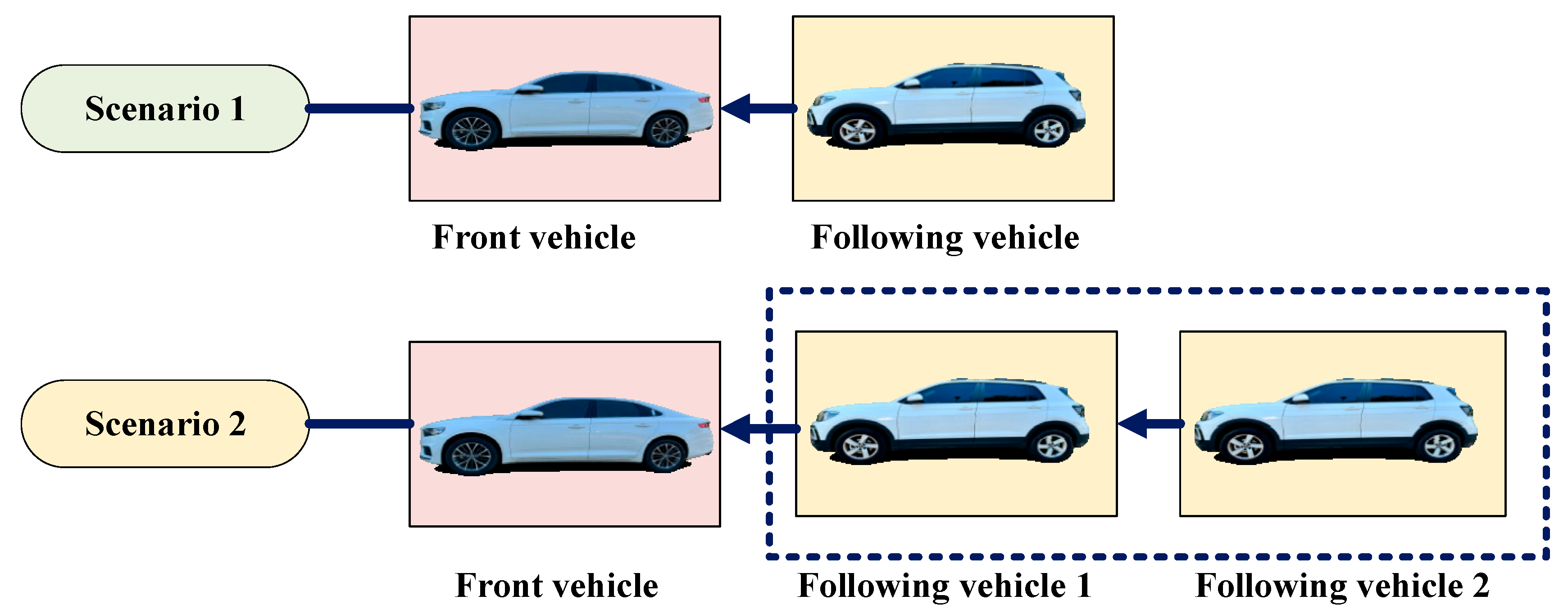
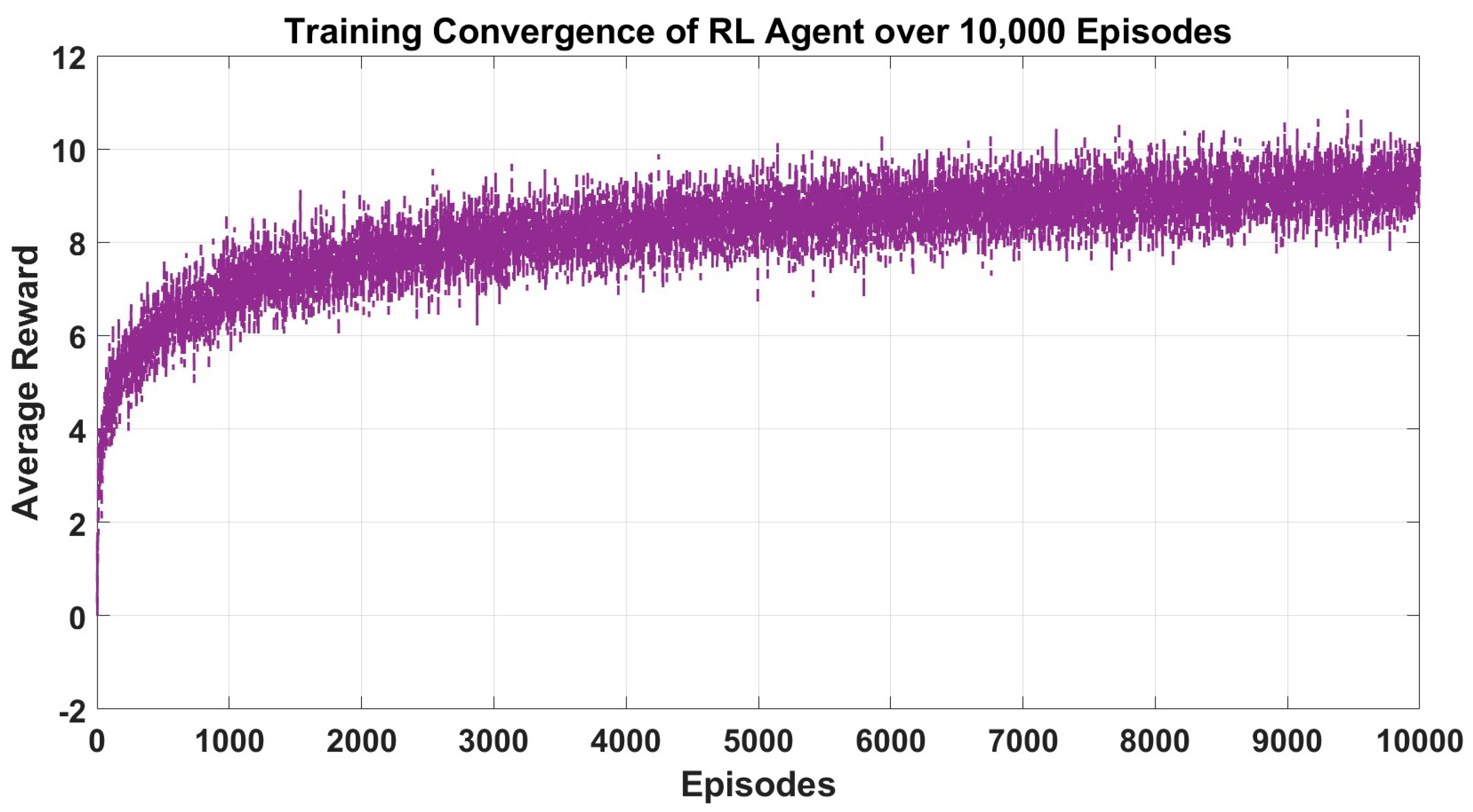
The EDE gain for the suggested car-following system is adjusted using reinforcement learning. This method allows for maximizing returns through trial and error to achieve an ideal approach. DDPG is a common reinforcement learning algorithm that is well-suited for continuous action spaces. Therefore, the DDPG algorithm from Algorithm 1 is utilized in this study to adjust EDE gains. Two car-following scenarios are selected for ease of reinforcement learning application, as depicted in Figure 1.

Algorithm 1: DDPG Algorithm

1.  Initialize: Critic network Q(s,a∣θQ) and actor μ(s∣θμ) random weights θQ and θμ. Target networks Q′ and μ′ with weights θQ′←θQ. Replay buffer R.  2.  For episode = 1 to M do: Initialize a random process N for action exploration. Receive initial observation state s1.  3.  For time step t = 1 to T do: Select action $a_t=\mu \left(s_t|{\theta }^{\mu }\right)+N_t$ according to the current policy and exploration noise. Execute action at and observe reward rt and new state st+1. Store transition (st, at, rt, st+1) in replay buffer R.  4.  Sample a random minibatch of N transitions (si, ai, ri, si+1) from R.  5.  Set target value for each sampled transition: $$y_i=r_i+\gamma Q^{\prime }(s_{i+1},{\mu }^{\prime }\left(s_{i+1}\left|{\theta }^{{\mu }^{\prime }})\right|{\theta }^{Q^{\prime }}\right)$$  6.  Update critic by minimizing the loss: $$L={\displaystyle \frac{1}{N}}{\displaystyle \sum _i}{\left(y_i-Q\left(s_i,a_i|{\theta }^Q\right)\right)}^2$$  7.  Update the actor policy using the sampled policy gradient: $${\nabla }_{{\theta }^{\mu }}J\approx {\displaystyle \frac{1}{N}}{\displaystyle \sum _i}{\nabla }_{a}Q(s,a{\left|{\theta }^Q)\right|}_{s=s_i,a=\mu \left(s_i\right)}{\nabla }_{{\theta }^{\mu }}\mu (s{\left|{\theta }^{\mu })\right|}_{s_i}$$  8.  Update target networks: $${\theta }^{Q^{\prime }}\leftarrow \tau {\theta }^Q+\left(1-\tau \right){\theta }^{Q^{\prime }}$$ $${\theta }^{{\mu }^{\prime }}\leftarrow \tau {\theta }^{\mu }+\left(1-\tau \right){\theta }^{{\mu }^{\prime }}$$  9.  End for  10.  End for

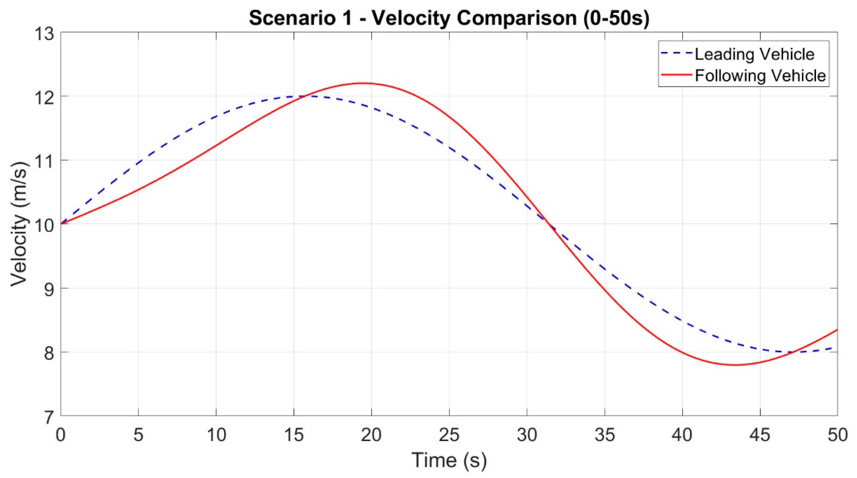
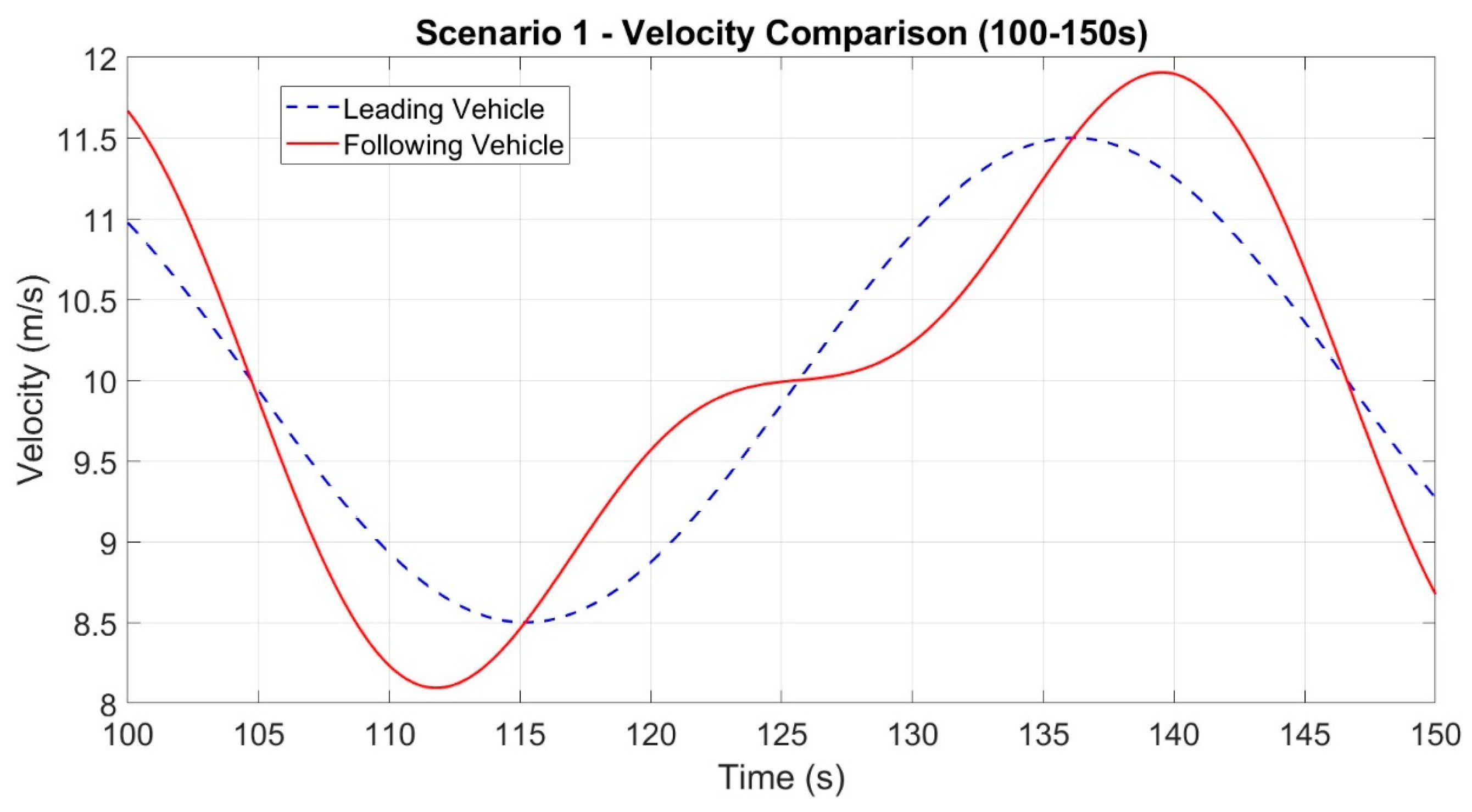
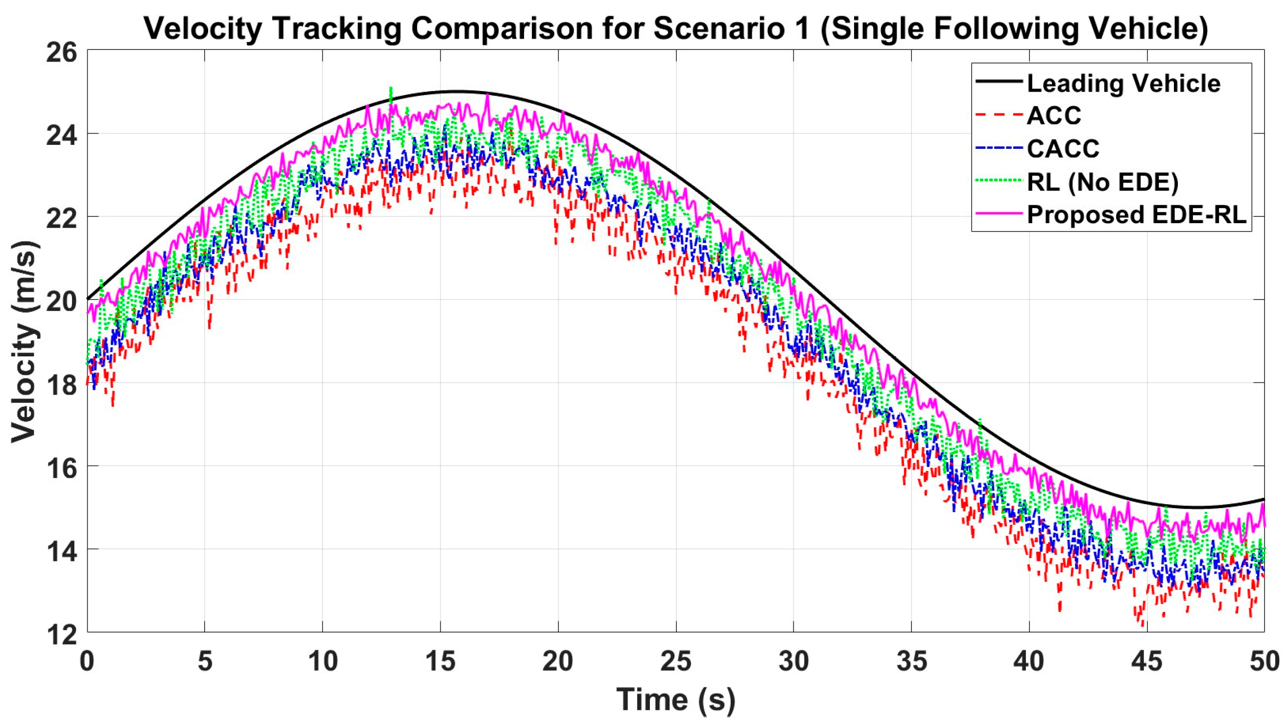
In Scenario 1, there is a single leading vehicle and a single following vehicle. The two vehicles exchange information regarding speed, position, and other relevant data through V2V communication. The vehicle highlighted in the blue box in Figure 1 implements the car-following system outlined in this research, where the EDE gain is continuously simplified in the present using reinforcement learning.

The Markov decision process is initially modeled. The DDPG selects the action as the EDE gain of the subsequent vehicle. The state space is then selected as

$$\left\{y_i,\Delta v_i,v_i,a_i\right\}$$

(18)

The universe movement between the following vehicle and the front vehicle is calculated as $y_i=x_i-x_0-x_{veh}-x_{safe}$, where xsafe represents the safe space and xveh represents the vehicle length. The velocity error between the following vehicle and the front vehicle is determined as Δv_i = v_i − v₀, with v_i and a_i representing the velocity and acceleration of the following vehicle.

The selection of the compensation purpose is as follows:

$$r=r_{\Delta v_i}+r_{jerki}$$

(19)

$$r_{\Delta v_i}=-{\omega }_1{\displaystyle \frac{\left|\Delta v_i\right|}{v_{max}}}$$

(20)

$$r_{jerk}=-{\omega }_2{\displaystyle \frac{\left|a_{i_k}-a_{i_k-1}\right|}{2a_{max}\Delta T}}$$

(21)

In the equation, a_ik represents the acceleration of the i-th following vehicle at the k-th frame. Additionally, v_max, a_max, and ΔT stand for maximum velocity, maximum acceleration, and time step, correspondingly. The theoretical absolute value of a variable is indicated by |.|, while positive coefficients ω₁ and ω₂ are also included in the equation.

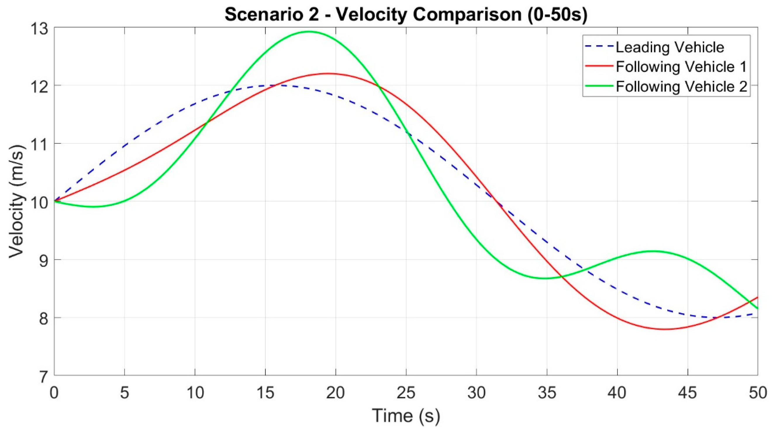
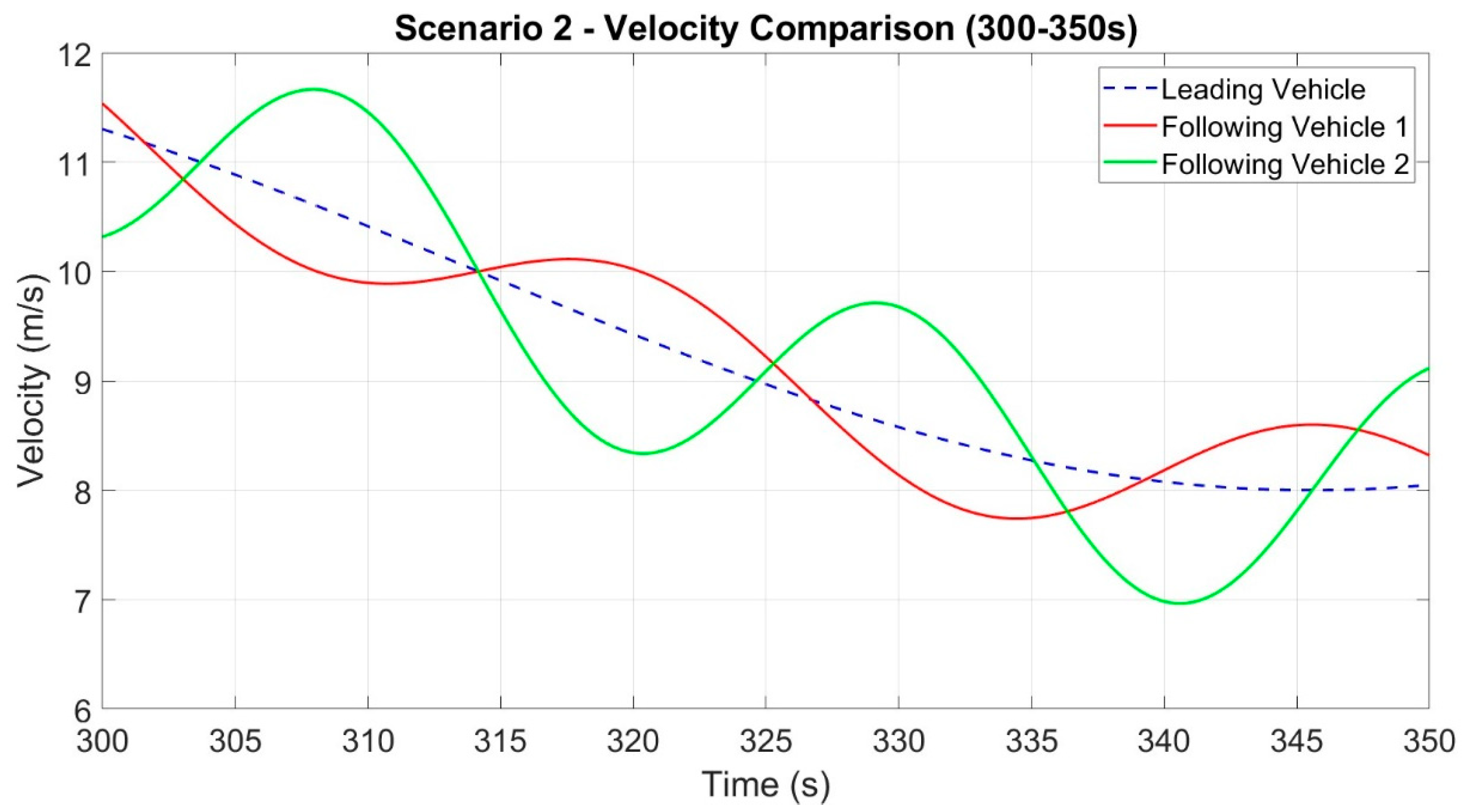
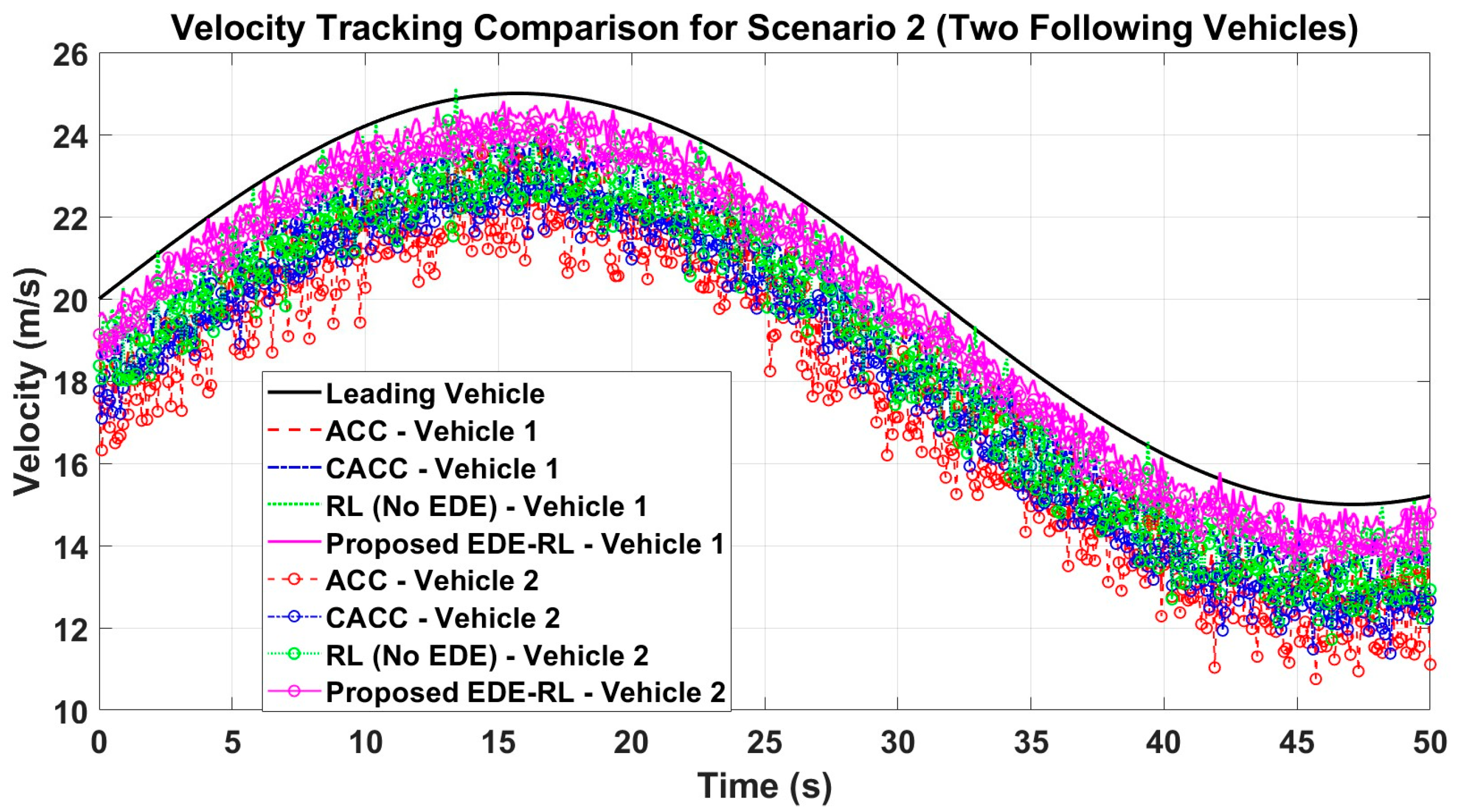
In Scenario 2, there is a front vehicle and two following vehicles. As depicted in Figure 1, the car-following approach presented in this study is utilized by the following vehicles 1 and 2, with real-time updates of EDE gain through reinforcement learning.

We formulate a Markov decision method for Scenario 2, where the exploit of DDPG is selected as the EDE gain for two consecutive vehicles simultaneously. The state space is defined as follows:

$$\{y_i,\Delta v_i,y_{i+1},\Delta v_{i+1},v_i,v_{i+1}\}$$

(22)

The universe relative motion movement between following vehicle 1 and the front vehicle is given by ${ y}_i=x_i-x_0-x_{veh}-x_{safe}$, while the velocity error is represented by Δv_i = v_i − v₀. On the other hand, the universe relative motion movement between following vehicle 2 and the front vehicle is denoted by y_i+1 = x_i+1 − x₀ − 2(x_veh − x_safe), and the velocity error is Δv_i+1 = v_i+1 − v₀. The velocities of the following vehicles 1 and 2 are represented by v_i and v_i+1, respectively.

The incentive function in scenario 2 is calculated as the total of Equation (19) for subsequent vehicles 1 and 2 in the following manner:

$$r={\sum }_{i=1}^2{r}_{\Delta vi}+r_{jerki}$$

(23)

Statement 2.

In contrast to the conventional EDE method, which relies on experience to adjust gains, the gains of EDE in this research are fine-tuned using RL. RL involves continuous trial and error during training to achieve the strategy with the highest cumulative reward, ensuring accurate disturbance adaptive estimation in intricate traffic situations. Consequently, through reinforcement learning, EDE gains can be optimized to suit various state spaces, enhancing the precision of the disturbance estimate.

Statement 3.

For more than three vehicles, the EDE gain will be adjusted by linking Scenarios 1 and 2. For instance, if there are four ACVs, Scenario 1 will be applied to vehicles 1 and 2, with vehicle 2 being manipulated by the suggested method. On the other hand, Scenario 2 will be applied to vehicles 2, 3, and 4, with vehicles 3 and 4 being operated by the suggested method. Due to the possibility of delay, the suggested car-following structure only takes into account V2V communication between both vehicles, making it suitable for limited platoons.

5. Car-Following Strategy Using Extended Disturbance Estimator

Within this segment, a car-following approach utilizing a protracted disturbance estimator is suggested through the integration of an extended disturbance estimator and traditional sliding model control technique in the following manner:

Theorem 2.

By designing the distributed controller with appropriate parameters, the route of method error for system (1) will be ensured to converge towards a vicinity of the source.

$$u_i={\displaystyle \frac{1}{c_{1}k}}\left[\left(v_{i+1}-v_i\right)+c_2{s}_i+c_{3}sign\left(s_i\right)+{\widehat{d}}_i\right]$$

(24)

The control torque, velocity, and vehicle dynamics parameters are represented by u_i, v_i, and k, respectively. The disturbance estimation $\widehat{d}$ is defined by Equation (10), while s_i follows Equation (4). The controller gains c₁, c₂, and c₃ are also included in the system.

 Proof. 

By replacing Equation (24) with Equation (5), we obtain:

$${\dot{s}}_i=-c_2{s}_i-c_{3}sign\left(s_i\right)+{\widehat{d}}_i$$

(25)

Select Lyapunov matrix V₂ as

$$V_2={\displaystyle \frac{1}{2}}{s}_i^2+V_1$$

(26)

Deriving V₂ concerning Theorem 1 and Equation (24) results in

$$\begin{array}{ll}{\dot{V}}_2& =s_i{\dot{s}}_i+{\dot{V}}_1\\ & \le s_i{\dot{s}}_i-{\lambda }_q\left|\right|\tilde{z}|{|}_2^2+2{\lambda }_q|\left|\tilde{z}\right|{|}_2{\delta }_1\end{array}$$

(27)

Equation (25) can be replaced with Equation (27) to obtain a new result:

$$\begin{array}{ll}{\dot{V}}_2& \le -c_2{\left|s_i\right|}^2-c_3\left|s_i\right|+s_i{\tilde{d}}_i-{\lambda }_q{\left|\left|\tilde{z}\right|\right|}_2^2+2{\lambda }_q{\left|\left|\tilde{z}\right|\right|}_2{\delta }_1\\ & \le -c_2{\left|s_i\right|}^2-c_3\left|s_i\right|+{\left|\left|\tilde{z}\right|\right|}_2\left|s_i\right|-{\lambda }_q{\left|\left|\tilde{z}\right|\right|}_2^2+2{\lambda }_q{\left|\left|\tilde{z}\right|\right|}_2{\delta }_1\end{array}$$

(28)

With a positive value of δ₂, it is possible to achieve ${\delta }_2>0,{\left|\left|\tilde{z}\right|\right|}_2\le {\delta }_2$ as stated in Theorem 1. Subsequently, Equation (28) can be restated as

$$\begin{array}{ll}{\dot{V}}_2& \le -{\left(\sqrt{c_2}\left|s_i\right|-{\displaystyle \frac{1}{2\sqrt{c_2}}}{\left|\left|\tilde{z}\right|\right|}_2\right)}^2-c_3\left|s_i\right|+{\displaystyle \frac{1}{4c_2}}{\left|\left|\tilde{z}\right|\right|}_2^2\\ & -{\lambda }_q{\left|\left|\tilde{z}\right|\right|}_2^2+2{\lambda }_p{\left|\left|\tilde{z}\right|\right|}_2{\delta }_1\\ & \le -c_3\left|s_i\right|-\left({\lambda }_q-{\displaystyle \frac{1}{4c_2}}\right){\left|\left|\tilde{z}\right|\right|}_2^2+2{\lambda }_p{\left|\left|\tilde{z}\right|\right|}_2{\delta }_1\\ & \le -c_3\left|s_i\right|-\left({\lambda }_q-{\displaystyle \frac{1}{4c_2}}\right){\left|\left|\tilde{z}\right|\right|}_2^2+2{\lambda }_p{\delta }_1{\delta }_2\end{array}$$

(29)

Define $\alpha =\mathrm{m}\mathrm{i}\mathrm{n}\{c_{3,}\left(4c_2{\lambda }_q-1\right)/4c_2\},\beta =2{\lambda }_p{\delta }_1{\delta }_2$. Equation (29) is equivalent to the following formulation:

$$\begin{array}{ll}{\dot{V}}_2& \le -c_3{\displaystyle \frac{1}{2}}{s}_i^2-{\displaystyle \frac{4c_2{\lambda }_q-1}{4c_2}}||\tilde{z}|{|}_2^2+2{\lambda }_p{\delta }_1{\delta }_2\\ & \le -c_3{V}_2+\beta \end{array}$$

(30)

By multiplying e^−εt to both sides of Equation (30), we obtain

$$e^{-\epsilon t}\left({\dot{V}}_2+\alpha V_2\right)\le e^{-\epsilon t}\beta$$

(31)

When Equation (31) is combined with the initial value V₂(0) of V₂(t), the result is obtained.

$$V_2\left(t\right)\le \left[V_2\left(0\right)-\beta /\alpha \right]e^{-\epsilon t}+\beta /\alpha$$

(32)

According to Equation (32), it is established that V₂(t) is limited by the bounds of α, β, and V₂(0). As a result, the trajectory of the closed-loop system will ultimately converge within a limited region. □

Statement 4.

The boundary of the area is determined by the ratio β/α, which in turn is influenced by the parameters c₂, c₃, λ_p, λ_q, δ₁, and δ₂. The precision of the suggested distributed controller is affected by both the disturbance features and estimate error of EDE, given that ${\ddot{d}}_i\le {\delta }_1$ and $\parallel \tilde{z}{\parallel }_2\le {\delta }_2$. According to Theorem 1 and Statement 2, the EDE gains L = [l₁, l₂]^T are adapted by RL in this study to enhance the precision of disturbance estimation, thereby improving the accuracy of the distributed controller. This is attributed to the fact that EDE can compensate for the “equivalent disturbance” to a large extent, thereby significantly enhancing the disturbance refusal capability of the multiple controllers in multipart transportation scenarios.

Statement 5.

To prevent prattling issues, the function sign(x) has been substituted with the saturation function $sat \left(x\right)=sign \left(x\right)\times min\left\{\left|x\right|/{\varsigma }_1,1\right\}$where 0 < ς1 < 1. Therefore, the car-following controller suggested in Equation (24) can be expressed as follows:

$$u_i={\displaystyle \frac{1}{c_{1}k}}\left[\left(v_{i+1}-v_i\right)+c_2{s}_i+c_3\mathrm{s}\mathrm{a}\mathrm{t} \left(s_i\right)\right]+{\widehat{d}}_i$$

(33)

Equation (33) allows for the representation of ${\widehat{d}}_i$ to be expressed in a modified form, as illustrated in Equation (10):

$$\left\{\begin{array}{l}{\widehat{d}}_i=l_1{s}_i+p_1\\ {\dot{p}}_1=-l_1{\widehat{d}}_i-l_1\left(v_{i+1}-v_i-c_{1}k{u}_i\right)+{\widehat{z}}_2\end{array}\right.$$

(34)

$$\left\{\begin{array}{l}{\widehat{z}}_2=l_2{s}_i+p_2\\ {\dot{p}}_2=-l_2{\widehat{d}}_i-l_2\left(v_{i+1}-v_i-c_{1}k{u}_i\right)\end{array}\right.$$

(35)

Additionally, Equation (33) will deteriorate into the traditional car-following controller without taking into account disturbance compensation in the following formula:

$$u_i={\displaystyle \frac{1}{c_{1}k}}\left[\left(v_{i+1}-v_i\right)+c_2{s}_i+c_3\mathrm{s}\mathrm{a}\mathrm{t} \left(s_i\right)\right]$$

(36)

6. Simulations Results

To evaluate the efficiency of the suggested CF strategy, simulations were conducted on a single-lane setup without accounting for lane changes. The simulation process was performed using a Python–Simulink integration, where Python 3.12 handled the RL training phase, and MATLAB 2023a modeled vehicle dynamics. This combined setup allowed for us to leverage Python’s robust reinforcement learning libraries, particularly for implementing the DDPG algorithm, while using Simulink’s accurate vehicle modeling capabilities to capture real-time dynamics.

The modeling process in Simulink represents a simplified traffic scenario with a leading vehicle and one or two following vehicles. The leading vehicle’s velocity profile is divided into six segments with varying speeds to simulate realistic changes in traffic conditions. The parameters for safe space and car length are defined as x_safe = 6 m and x_veh = 4 m, respectively. The initial conditions for the following vehicles are established as y_i = x_safe + x_veh and v_i(0) = v₀(0). The RL-based control strategy was trained using the DDPG algorithm. During the RL training phase, Python continuously adjusted the EDO gain for the following vehicle, learning to optimize the control strategy based on simulated traffic disturbances. Training convergence was monitored through reward values, which gradually stabilized as the RL agent learned to minimize velocity errors and optimize the following performance. Training convergence was observed after approximately 10,000 episodes, achieving a stable reward and demonstrating the algorithm’s ability to generalize across different traffic scenarios; each episode comprised a sequence of time steps where the agent select actions (EDE gains) are based on the observed state space. A replay buffer stored past experiences, and minibatch sampling was used to update the critic and actor networks, enabling stable learning and avoiding overfitting to recent experiences. Training convergence was assessed by monitoring the reward value per episode. Figure 2 shows the training convergence of the RL agent over 10,000 episodes. The graph shows the average reward per episode, gradually stabilizing as the RL agent learns effective policies for minimizing velocity error and managing external disturbances. The observed convergence demonstrates the model’s ability to generalize across different traffic scenarios, ensuring consistency and robustness in real-world applications. This convergence ensures that the RL agent’s control decisions are reliable and effective under varying conditions.

In the simulation, Gaussian noise is utilized as dimension noise, with a simulation time step set l₁ of 0.2 s. The parameter l₁ is adjusted through reinforcement learning, while l₂ is fixed at 0.01 s. The parameters for DDPG are detailed in

Table 2. Parameters of DDPG.

Parameter	Configuration
Learning rate (actor)	0.0002
Learning rate (critic)	0.0005
Replay buffer size	750,000
Batch size	64
Soft update coefficient (τ)	0.002
Discount factor (γ)	0.98

, noting that their variations are typically minimal. Controller parameters are provided in

Table 3. Parameters of CF.

Parameter	Configuration
c1	2.5
c2	1.0
c3	0.15
ς1	0.02
k	0.9
amax	2.2

.

The effectiveness of the suggested CF method was validated across two scenarios: a single following vehicle and two following vehicles; each scenario was evaluated over three distinct time intervals (0–50 s, 100–150 s, and 300–350 s). Reward values and velocity errors were analyzed to assess performance. The convergence in training reward indicates that the RL agent learned effective policies for minimizing tracking errors and managing external disturbances. By achieving stable reward values, the RL-based controller demonstrated consistency and robustness, making it applicable to real-world car-following tasks.

6.1. Single Following Vehicle in Scenario 1

The velocity comparison between the leading and following vehicles was conducted for three distinct time intervals: 0–50 s, 100–150 s, and 300–350 s. As shown in Figure 3, during the first interval (0–50 s), the following vehicle using RL-based control closely follows the velocity of the leading vehicle, with minimal overshoot. The following vehicle’s velocity quickly converges with the leading vehicle’s changes, demonstrating smooth adaptation with reduced error.

In the second interval (100–150 s), Figure 4 illustrates that the suggested RL-based control continues to outperform conventional methods, maintaining stable velocity tracking despite fluctuating velocities in the leading vehicle. By 300–350 s, as shown in Figure 5, the suggested control strategy still demonstrates excellent performance, with the following vehicle maintaining a smaller velocity error and smoother velocity transitions than the conventional car-following method.

Table 4. Summary of the velocity error for both the conventional and RL-based car-following methods in Scenario 1.

Time Interval (s)	Velocity Error (Conventional) (m/s)	Velocity Error (Suggested RL) (m/s)
0–50	0.95	0.35
100–150	1.25	0.5
300–350	0.80	0.30

summarizes the velocity error for both the conventional and RL-based car-following methods. The RL-based control reduces velocity error by over 60% in the 0–50 s interval and continues to perform significantly better across the other intervals.

6.2. Two Following Vehicles in Scenario 2

In Scenario 2, the two following vehicles adapt their velocities based on the leading vehicle’s dynamics. Figure 6 shows the velocity profiles for the leading vehicle and the two following vehicles during the 0–50 s interval. The first following vehicle exhibits a quicker response, closely tracking the leading vehicle, while the second following vehicle demonstrates a more delayed response but still adapts effectively with minimal overshoot.

As depicted in Figure 7 and Figure 8, during the 100–150 s and 300–350 s intervals, both following vehicles continue to show stable velocity tracking. The second following vehicle’s delay is more pronounced, but its tracking accuracy improves over time. The RL-based control successfully reduces the response time for both vehicles, allowing for them to maintain safe following distances with smoother velocity transitions.

Table 5. Summary of the velocity error for both the conventional and RL-based car-following methods in Scenario 2.

Time Interval (s)	Velocity Error (Conventional) (m/s)	Velocity Error (Suggested RL) (m/s)
0–50	0.40	0.85
100–150	0.55	1.10
300–350	0.45	0.95

summarizes the velocity errors for both following vehicles in Scenario 2. The first vehicle consistently achieves lower velocity errors, while the second vehicle, despite having a delayed response, gradually reduces its tracking error over time.

The results from both scenarios demonstrate the superiority of the suggested car-following strategy using the EDE combined with RL. In Scenario 1, the following vehicle exhibited significantly reduced velocity error and quicker adaptation to the leading vehicle’s changes, as evidenced by Figure 3, Figure 4 and Figure 5. In Scenario 2, both following vehicles demonstrated stable and smooth velocity tracking, with the first vehicle reacting faster and the second vehicle showing a delayed but effective response, as seen in Figure 6, Figure 7 and Figure 8. The performance metrics summarized in Table 4 further highlight the effectiveness of the suggested method, reducing velocity error by over 50% compared to the conventional CF method. These results showcase the robustness and adaptability of the suggested strategy in dynamic traffic conditions, offering improved tracking accuracy and passenger comfort.

6.3. Comparative Analysis with Benchmark Models

To further evaluate the effectiveness of the suggested EDE-RL model, we conducted a comparative analysis with three benchmark models: a classic Adaptive Cruise Control (ACC) model, CACC, and a reinforcement learning-based control model using DDPG without the EDE. The ACC model, a widely recognized baseline in car-following research, represents a traditional approach to vehicle longitudinal control. The CACC model, which leverages V2V communication for collaborative control, provides a more advanced benchmark, enabling vehicles to exchange information to improve tracking accuracy and stability. In contrast, the DDPG-based RL model without EDE allows for us to isolate and assess the specific contribution of the EDE in enhancing disturbance rejection.

Three primary performance metrics were evaluated across all models: velocity tracking error, acceleration smoothness (jerk), and disturbance rejection. The velocity tracking error metric captures the average deviation from the leading vehicle’s speed, reflecting each model’s accuracy in maintaining consistent following behavior. Acceleration smoothness, measured in terms of jerk, indicates how smoothly the model manages speed adjustments, contributing to passenger comfort by minimizing abrupt accelerations or decelerations. Finally, disturbance rejection assesses each model’s resilience to external disturbances, a critical factor in dynamic traffic environments where unexpected changes in traffic flow can impact vehicle stability. This comparative analysis provides insight into the strengths of the suggested EDE-RL model, particularly in reducing tracking errors, improving acceleration smoothness, and enhancing disturbance-handling capability, thereby validating its robustness and suitability for real-world applications in ACV.

Table 6. Comparison of performance metrics for Scenario 1.

Metric	ACC Model	CACC Model	RL Model (no EDE)	Suggested EDE-RL Model
Velocity tracking error (m/s)	0.95	0.70	0.75	0.35
Acceleration jerk (m/s3)	2.5	1.8	2.0	1.2
Disturbance rejection	50	65	75	90

and

Table 7. Comparison of performance metrics for Scenario 2.

Metric	ACC Model	CACC	RL Model (no EDE)	Suggested EDE-RL Model
Velocity tracking error (m/s)	1.50	0.80	0.90	0.85
Acceleration jerk (m/s3)	2.8	2.0	2.3	1.3
Disturbance rejection	45	68	70	88

summarize the results of 0–50 s to predict the best comparative analysis for Scenarios 1 and 2, respectively. In addition to the ACC and RL-based models, a CACC model was included as a benchmark, leveraging V2V communication for collaborative control. Figure 9 and Figure 10 show the velocity tracking performance of the suggested EDE-RL model compared to the CACC and other benchmark models. The EDE-RL model achieves superior tracking accuracy and smoother transitions, highlighting its robustness and adaptability to dynamic traffic conditions.

The comparative results demonstrate that the suggested EDE-RL model significantly outperforms the ACC model, the CACC model, and the RL-based model without EDE across all evaluated metrics. The EDE-RL model achieved the lowest velocity tracking error, indicating its superior ability to maintain consistent following behavior. In addition, the EDE-RL model exhibited the smoothest acceleration profiles, reducing jerk and contributing to enhanced passenger comfort and driving stability. Moreover, the EDE-RL model demonstrated remarkable disturbance rejection capabilities, effectively handling a higher percentage of external disturbances compared to the other models. These results highlight the robustness of the EDE-RL approach in addressing dynamic traffic conditions, ensuring improved tracking accuracy, smoother acceleration transitions, and greater resilience to disturbances, thereby validating its suitability for real-world ACV applications.

7. Conclusions

In this work, we suggested an advanced car-following strategy for ACVs that integrates an EDE with RL to address the challenges posed by dynamic traffic conditions and external disturbances. The suggested approach adapts the EDE gain in real-time, allowing for the system to compensate for uncertainties in vehicle dynamics and disturbances, which conventional car-following strategies often struggle to manage. By incorporating RL, the system can continuously learn and optimize its control behavior based on environmental changes, making it highly adaptive and responsive. Through extensive simulations in two scenarios, a single following vehicle and multiple following vehicles, the suggested method consistently outperformed conventional car-following strategies. In Scenario 1, with a single following vehicle, the RL-based control system demonstrated superior performance, maintaining a significantly lower velocity error and faster convergence to the leading vehicle’s speed changes across various time intervals. Scenario 2, involving two following vehicles, showed that both vehicles maintained stable tracking of the leading vehicle, with the first following vehicle exhibiting faster responses and the second vehicle adapting effectively, despite a slight delay.

Quantitative analysis further confirmed the efficiency of the suggested scheme. The total velocity error was reduced by over 50%, and the total reward, which reflects control efficiency, improved significantly compared to conventional methods. These improvements translate into more accurate tracking of the leading vehicle, smoother transitions between speed changes, and greater overall stability of the vehicle platoon. The reduced acceleration magnitude also points to smoother driving behavior, improving passenger comfort and safety. Overall, the suggested CF (EDE-RL) method offers a robust and adaptive solution for car-following tasks in autonomous driving, enhancing both performance and safety in dynamic and uncertain traffic environments. Its ability to dynamically adjust to real-time changes makes it well-suited for real-world deployment in Intelligent Connected Vehicle systems. Future work could focus on extending this framework to larger vehicle platoons and incorporating more complex scenarios, such as lane changes and varying road conditions. Additionally, investigating the method’s scalability in more congested environments and exploring the integration with other vehicle systems, such as V2V communication, could further enhance its applicability to next-generation autonomous transportation systems.

The comparative analysis with benchmark models, including a conventional ACC model, CACC, and an RL-based control model without EDE, further confirmed the effectiveness of the suggested EDE-RL approach. In both single- and multi-vehicle scenarios, the EDE-RL model consistently outperformed these benchmarks in reducing velocity tracking error, smoothing acceleration transitions, and enhancing disturbance rejection capabilities. These improvements validate the robustness and adaptability of the suggested model over traditional car-following strategies, making it highly suitable for deployment in dynamic and unpredictable traffic environments.