Cross-Shaped Peg-in-Hole Autonomous Assembly System via BP Neural Network Based on Force/Moment and Visual Information

Abstract

Currently, research on peg-in-hole (PiH) compliant assembly is predominantly limited to circular pegs and holes, with insufficient exploration of various complex-shaped PiH tasks. Furthermore, the degree of freedom for rotation about the axis of the circular peg cannot be constrained after assembly, and few studies have covered the complete process from autonomous hole-searching to insertion. Based on the above problems, a novel cross-shaped peg and hole design has been devised. The center coordinates of the cross-hole are obtained during the hole-searching process using the three-dimensional reconstruction theory of a binocular stereo vision camera. During the insertion process, 26 contact states of the cross-peg and the cross-hole were classified, and the mapping relationship between the force-moment sensor and relative errors was established based on a backpropagation (BP) neural network, thus completing the task of autonomous PiH assembly. This system avoids hand-guiding, completely realizes the autonomous assembly task from hole-searching to insertion, and can be replaced by other structures of pegs and holes for repeated assembly after obtaining the accurate relative pose between two assembly platforms, which provides a brand-new and unified solution for complex-shaped PiH assembly.

1. Introduction

As the last process of modern manufacturing, mechanical assembly has a direct impact on product quality. In the era of Industry 5.0 [1,2,3], robots are extensively utilized in modern industrial manufacturing fields, such as those of computer, communication and consumer electronics (3C) [4] manufacturing, automobile assembly [5], and reducer installation [6].

However, most robots are limited to position-controlled operations, such as gripping, placing, and painting [7]. They lack the flexibility and perception required for precision work like peg-in-hole (PiH) assembly [8], welding [9,10], and grinding. Additionally, autonomous planning and decision-making abilities are necessary for such tasks. Therefore, force sensors [11,12] are typically installed at the end of a robot to enable real-time motion adjustment based on force-moment information from the sensors. This technology is known as active flexible assembly technology, and the PiH task represents a typical application of this approach.

The PiH task can be divided into two primary processes: hole-searching and insertion. During the hole-searching phase, conventional techniques, such as Archimedean spiral search [13], grid search [14], and random search [15], are commonly employed in blind searches. The blind search method using force sensors may require extensive time and distance during the search phase, potentially exacerbating issues associated with such a technique. As a result, visual servoing is frequently utilized in PiH tasks [16]. Visual servoing can partially address the issue of difficult assembly convergence caused by position errors [17]. However, the introduction of visual servoing increases the amount of information to be processed. Therefore, machine learning is applied in the field of vision-based PiH assembly [18,19].

Chang implemented a dynamic visual servo-based miniature PiH assembly method [20]. The PiH task is the most intricate process in assembly, encompassing several key components such as robotic trajectory planning, peg and hole contact state determination, and pose adjustment. As a result, numerous scholars have integrated machine learning into PiH tasks to emulate human operations through reinforcement learning [21,22], convolutional neural networks [23], piecewise strategies, hierarchical learning [24] and decoupling control [25].

However, the current PiH assembly tasks are predominantly limited to circular peg and hole assembly, with research on shaped-PiH assembly still in its infancy. Song carried out complex-shaped PiH assembly under the teaching mode of a robot [26], while Park experimented with circular, triangular, and square PiH assembly using a manipulator [27]. However, they all used the blind searching method, which is less efficient. Li employed a multi-stage search method to perform PiH assembly with irregular shapes under partial constraints; yet, this approach failed to achieve the precise relative pose of the two assembly platforms and lacks universality [28].

To avoid having too many training samples for neural networks, which can damage the device, it is transformed into a regression problem [29], combining vision and force perception to complete the assembly of 16 kinds of sockets. Ahn completed the PiH assembly task for square, star, and double cylinder shapes through blind search using deep reinforcement learning algorithms. This study used hand-guiding to initially locate the assembling surface, so that the robotic arm only had to perform the insertion task. However, this design overlooks a crucial aspect: the most difficult point of automated PiH assembly is allowing the robotic arm to find the location of the hole with eyes (visual servoing) and to use hands (force sense) like a human to adjust the peg’s angle, position, and speed for smooth insertion into the hole. If human intervention is used to guide the peg near the hole, then the entire assembly system also intervenes in the intelligent body and greatly reduces subsequent insertion difficulties. This assembly strategy goes against the original purpose of automated assembly.

The aim of this paper is to devise a novel and versatile autonomous assembly mechanism for PiH tasks, as obtaining the pose presents a significant challenge in PiH assembly. Once the precise relative pose between the two assembly platforms is obtained, the robotic arm can easily replicate the PiH operation. Due to the ability of a circular peg to rotate around its axis even after assembly, achieving precise positional alignment between the working end and the fixed end of the robot is unattainable. Therefore, it is necessary to design a peg that constrains circumferential rotation.

The new assembly strategy allows for the replacement of pegs and holes of any shape once cross-shaped peg-in-hole assembly has been achieved, without the need to reformulate the assembly strategy or design specialized sensors. Only calibration of the robotic arm and the sensor is required to reproduce the research content presented in this paper and obtain the relative pose between the peg and the hole. This feature allows for the replacement of the shapes and sizes of the pegs and holes while maintaining proper functionality, thereby reducing the workload of users and improving industrial production efficiency.

2. Binocular Stereo Vision Based Hole-Searching

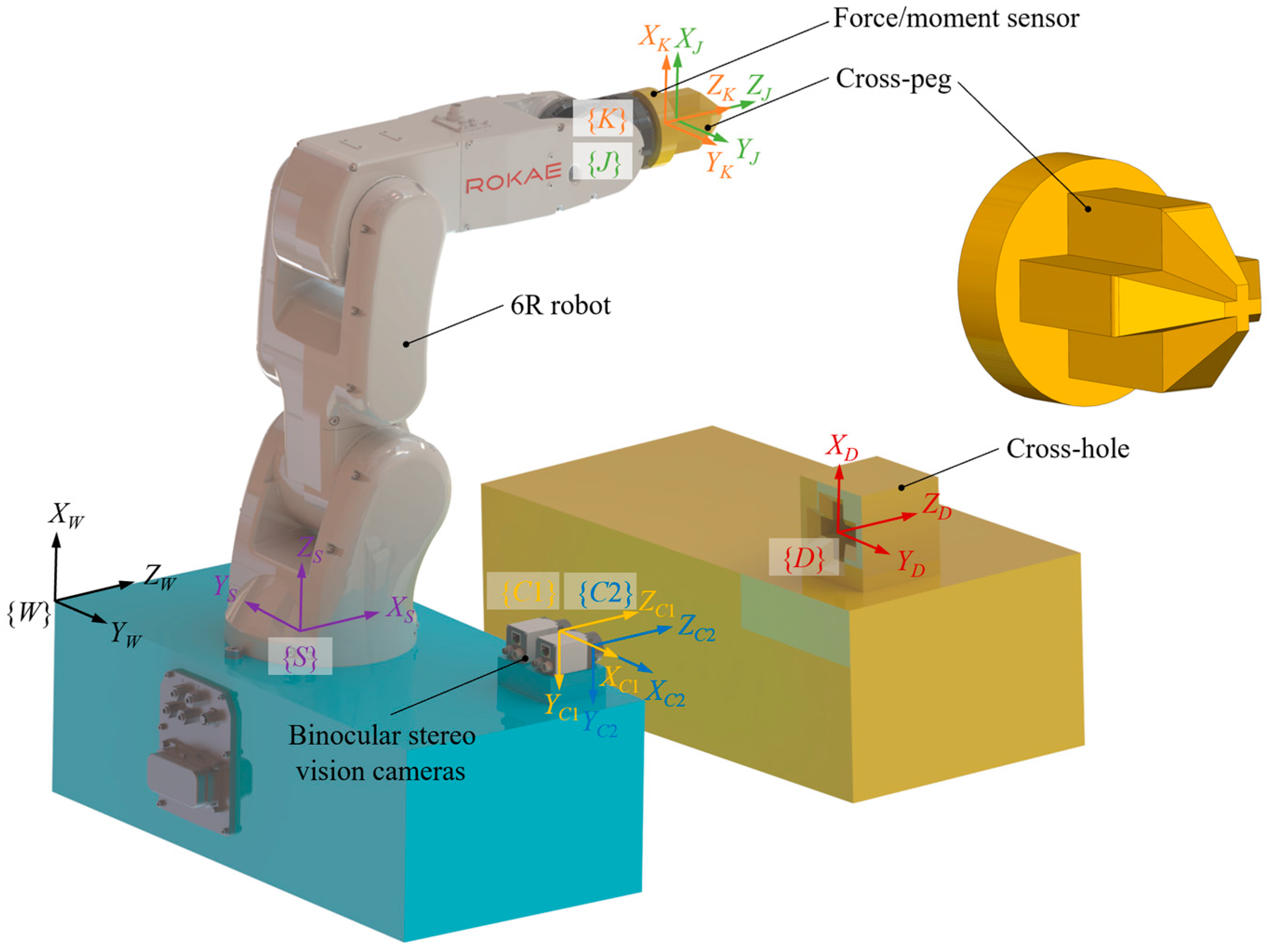
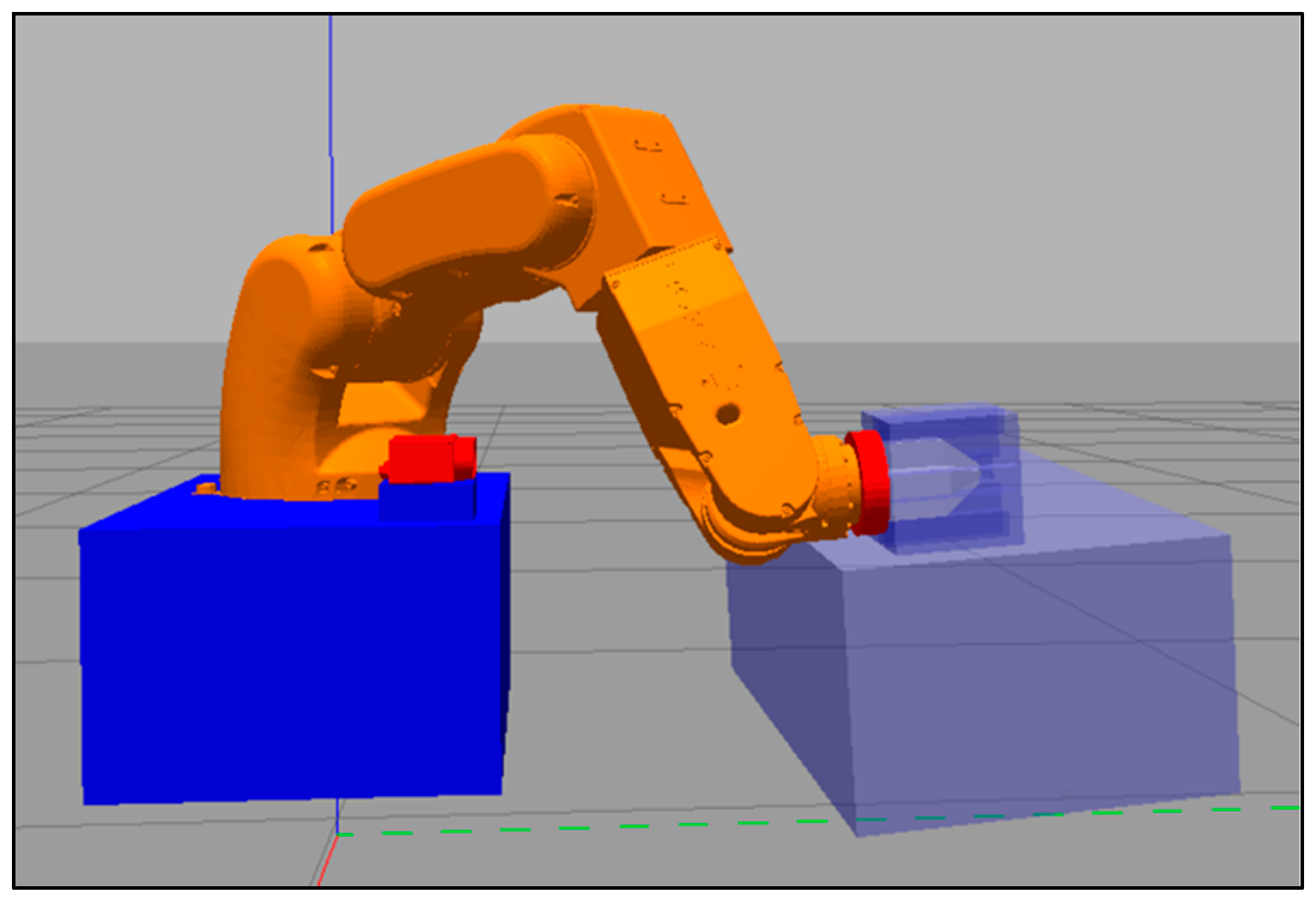
Responding to the current problems in PiH assembly, a novel assembly strategy is proposed that utilizes a binocular camera to determine the center coordinates of the cross-hole [30,31]. This enables the robot to autonomously locate the hole without requiring manual guidance. This autonomous assembly system consists of a 6R robot, a force-moment sensor, a cross-shaped feedback peg, a cross-shaped hole, and a binocular camera, as shown in Figure 1; {J} is the cross-peg coordinate system, {K} is the sensor coordinate system, {S} is the robot base coordinate system, {C1} is the left camera coordinate system, {C2} is the right camera coordinate system, {D} is the cross-hole coordinate system, and {W} is the actual world coordinate system.

The cross-section of the cross-peg and cross-hole is cross-shaped, which effectively constrains the rotation degrees of freedom (DoF) about the x, y, and z axes and the translation DoF about the x and y axes at the same time after completing the assembly. This limits the end joint of a 6R robot to 5 DoF, addressing the issue that the rotation DoF about the z-axis cannot be constrained by a circular peg. Meanwhile, the cross-peg features a tapered end, and the front of the cross-hole is chamfered. The tapered design reduces the requirement for the accuracy of the initial positioning using the binocular camera and solves the problem that the assembly of the circular peg is prone to failures of convergence.

The 6R robot and the binocular camera are fixed on the same platform, with a force-moment sensor and a cross-shaped feedback peg connected in series at the end of the robot, and the cross-hole is fixed on another assembly platform. A binocular stereo vision system was constructed using two monocular industrial cameras, specifically the JAI Go-X model. The binocular vision camera can capture the coordinates of the cross-hole center, and the force-moment sensor can collect the force/moment information during the assembly process, which can be combined with machine learning to train the robot to complete the autonomous PiH task. Based on the required arm reach and the workload of the robot, the ROKAE XB4 series industrial robot was selected as the 6R robot for this research project. This particular model features a payload capacity of 4 kg, an arm reach of 596 mm, and a positioning repeatability of ±0.02 mm.

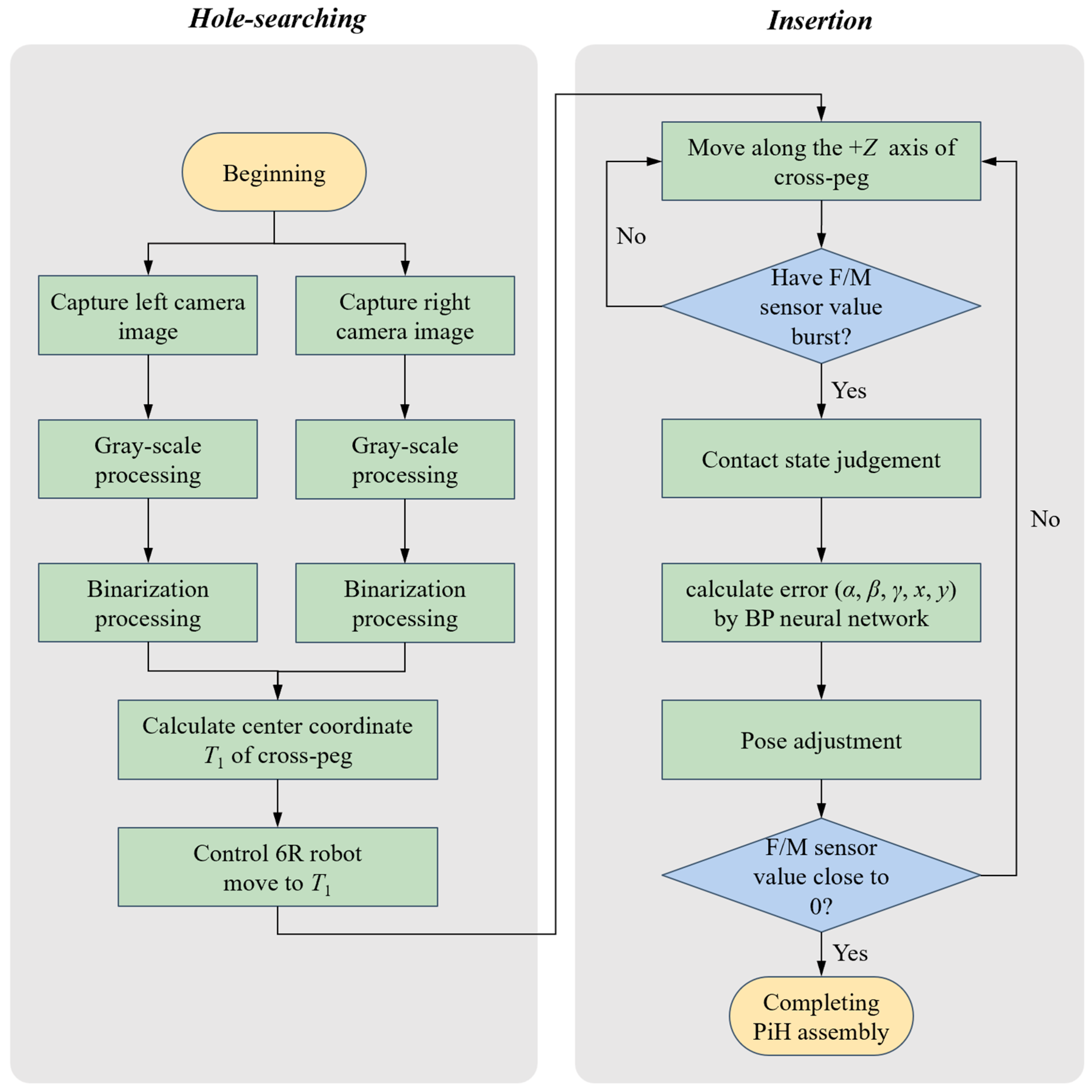
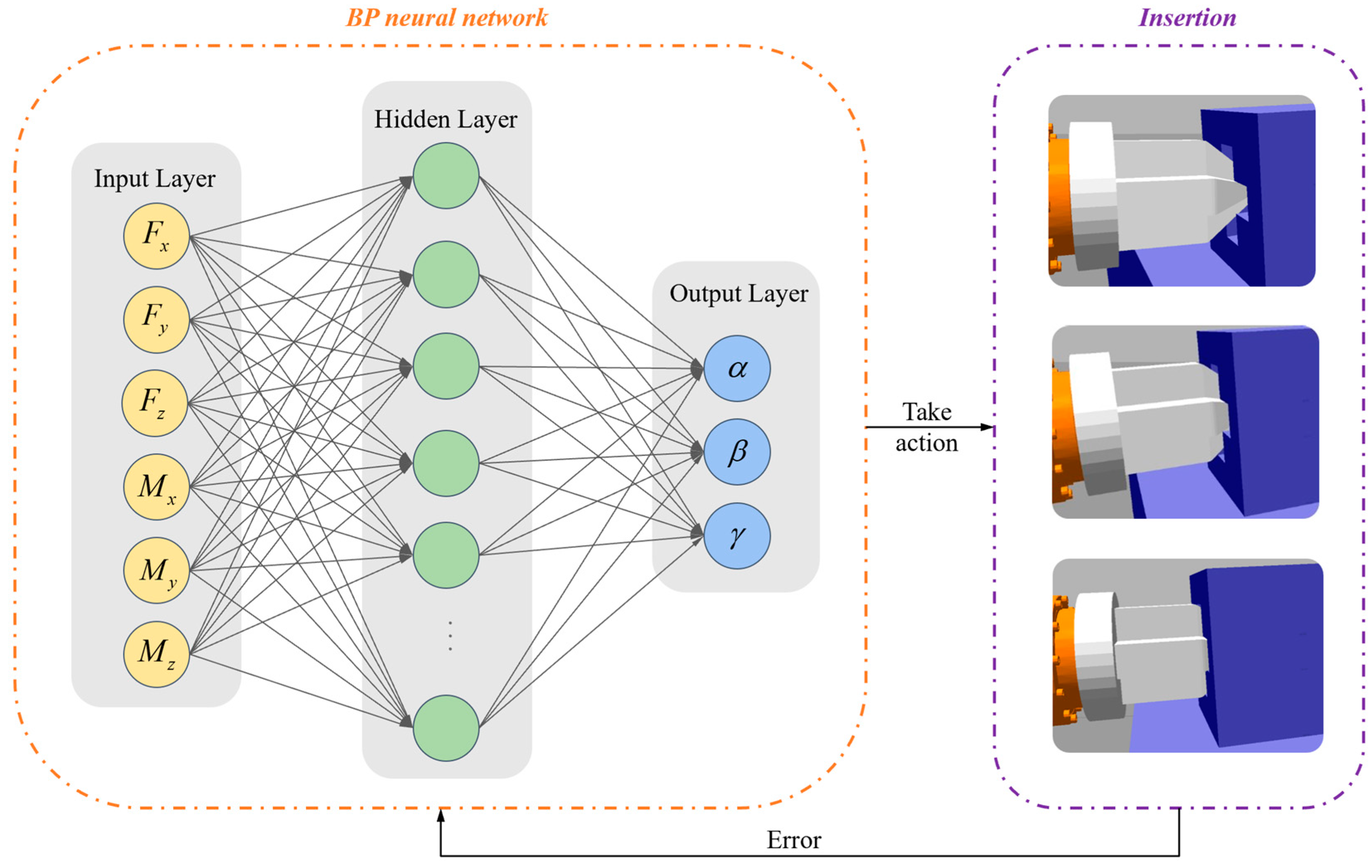
In this study, the Robot Operating System (ROS) was selected as the development platform due to its capability of achieving 3D visualization and motion simulation. By integrating MATLAB for data processing and backpropagation (BP) neural network training, the ROS system can efficiently accomplish autonomous assembly tasks. The PiH assembly flowchart is shown in Figure 2. This flowchart shows that the autonomous assembly system is divided into two processes: hole-searching and insertion. In the hole-searching process, the binocular camera image processing and the calculation of the center coordinate of the cross-hole are mainly carried out. In the insertion process, the 26 contact states are judged based on force-moment sensor values, and then the pose error is calculated using the BP neural network. This iterative process continues until PiH assembly is completed.

2.1. Feature Extraction for Cross-Peg

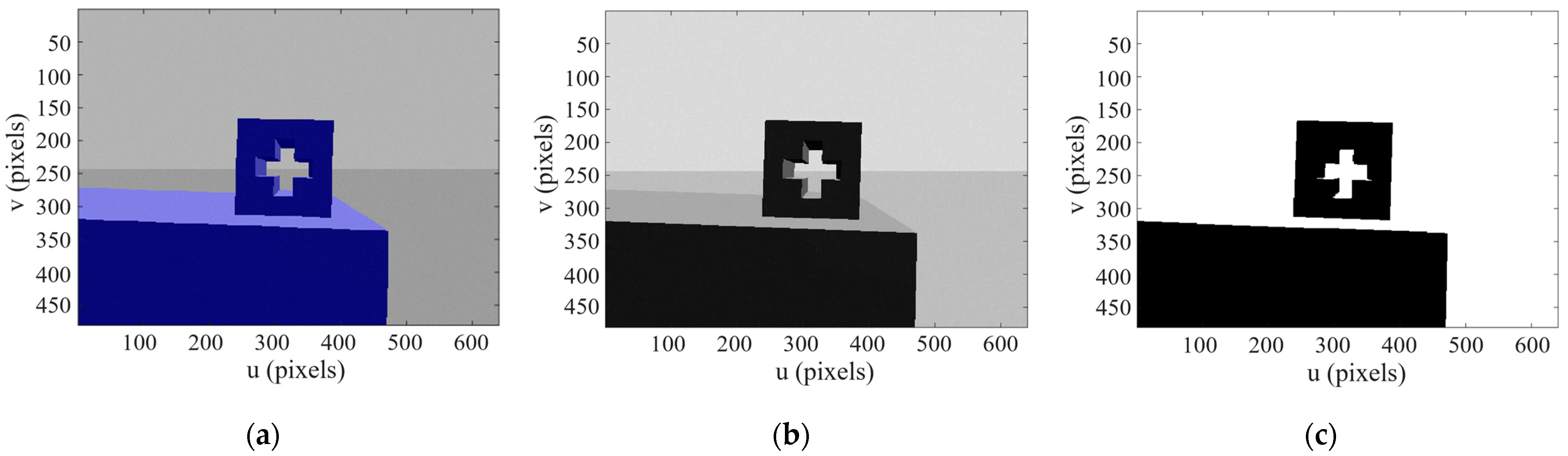
To calculate the pose of the cross-hole coordinate system relative to the robot base coordinate system {S}, it is necessary to perform image processing first in order to identify the cross-hole features. Then, based on the principle of 3D reconstruction by binocular vision, the spatial coordinates of the center of the cross-hole are obtained. The image of the cross-hole captured by the binocular stereo vision camera is shown in Figure 3a. After obtaining the image, the method of gray-scale classification [32,33] is used to extract features of the image. Figure 3b displays the image after undergoing gray-scale processing.

The grayscale image’s pixels are binarized into black and white based on a predetermined threshold value t. The pixel type is set to 0 when the grayscale value of the pixel is less than t; the pixel type is set to 1 when the grayscale value of the pixel is greater than t:

$$c\left(u,v\right)=\left\{\begin{array}{ll}0& I\left(u,v\right)<t\\ 1& I\left(u,v\right)\ge t\end{array}\right.\begin{array}{c}\forall \left(u,v\right)\in I\end{array}$$

(1)

where c is the pixel type, represented by an integer, I is the grayscale value of each pixel point in the grayscale image, in the range 0 to 1, t is the threshold value, and after binarization, the value of 1 represents the background and is displayed in white, while the value of 0 represents the target after binarization process and is displayed in black.

Figure 3c shows the image after the binarization process. Since the cross-hole is a through hole, the cross-hole is shown as a white cross shape surrounded by black annulus in the binarized image.

2.2. Calculation of Three-Dimensional Center Coordinates of the Cross-Hole

The monocular camera solely captures the planar information of an object while losing its depth perception. Therefore, a parallel binocular stereo vision camera is employed to simultaneously gather information from two views and the parallax ranging method is utilized for 3D reconstruction [34] of spatial points, ultimately obtaining the 3D coordinates of the cross-hole’s center [35].

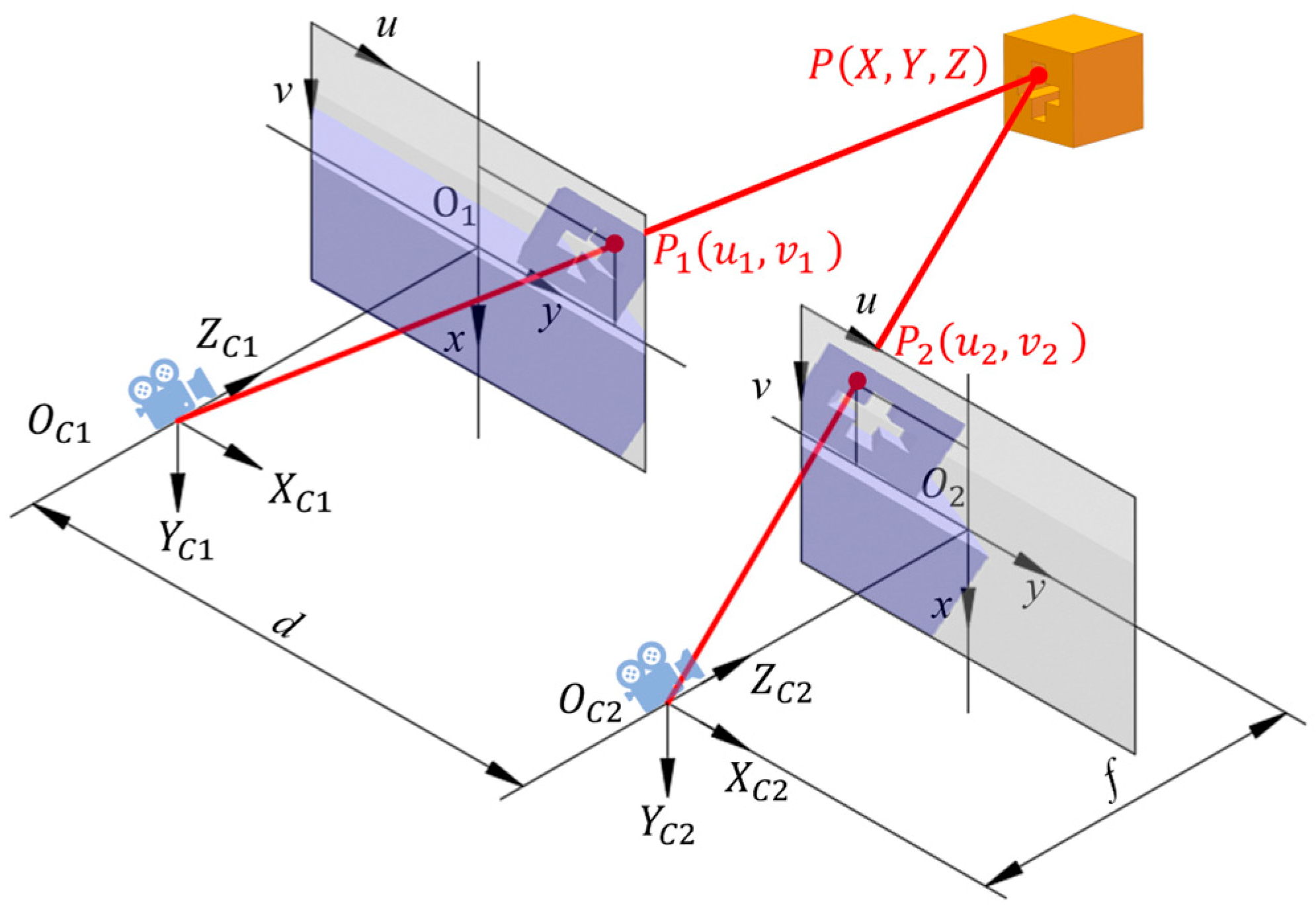
As illustrated in Figure 4, the operational principle of binocular stereo vision [36] involves two camera coordinate systems: {C1} for the left camera with $O_{C1}-X_{C1}{Y}_{C1}{Z}_{C1}$, and {C2} for the right camera with $O_{C2}-X_{C2}{Y}_{C2}{Z}_{C2}$. Both cameras have a focal length f and parallel optical axes separated by a fixed distance d. The binocular cameras utilized in this study have a focal length of 381.2612 mm.

Point P is projected onto the left camera at $P_1(u_1,v_1)$ and onto the right camera at $P_2(u_2,v_2)$, then the point P is located at the intersection of the line $O_{C1}{P}_1$ and the line $O_{C2}{P}_2$. The coordinates of the point P in the coordinate system {C1} are $(x_{C1},y_{C1},z_{C1})$ and in the coordinate system {C2} are $(x_{C2},y_{C2},z_{C2})$; then, the relationship between the two coordinate systems {C1} and {C2} is

$$\left\{\begin{array}{l}{x}_{C1}=x_{C2}+d\\ y_{C1}=y_{C2}\\ z_{C1}=z_{C2}\end{array}\right.$$

(2)

The coordinates of imaging points $P_1$ and $P_2$ in the image coordinate system $(x_1,y_1)$ and $(x_2,y_2)$ can be obtained according to Equation (2), and the relationship between the image coordinate system and the camera coordinate system can be determined by applying the principle of similar triangles:

$$\left\{\begin{array}{c}{\displaystyle \frac{f}{z_{C1}}}={\displaystyle \frac{x_1}{x_{C1}}}={\displaystyle \frac{y_1}{y_{C1}}}\\ {\displaystyle \frac{f}{z_{C2}}}={\displaystyle \frac{x_2}{x_{C2}}}={\displaystyle \frac{y_2}{y_{C2}}}\end{array}\right.$$

(3)

Simultaneously with Equations (2) and (3), the spatial coordinate $(x_{C1},y_{C1},z_{C1})$ of the point P in the left camera coordinate system {C1} is obtained as

$$\left\{\begin{array}{l}{x}_{C1}={\displaystyle \frac{x_1}{f}}{z}_{C1}={\displaystyle \frac{x_1}{x_1-x_2}}d\\ y_{C1}={\displaystyle \frac{y_1}{f}}{z}_{c1}={\displaystyle \frac{y_1}{y_1-y_2}}d\\ z_{C1}={\displaystyle \frac{f\cdot d}{x_1-x_2}}\end{array}\right.$$

(4)

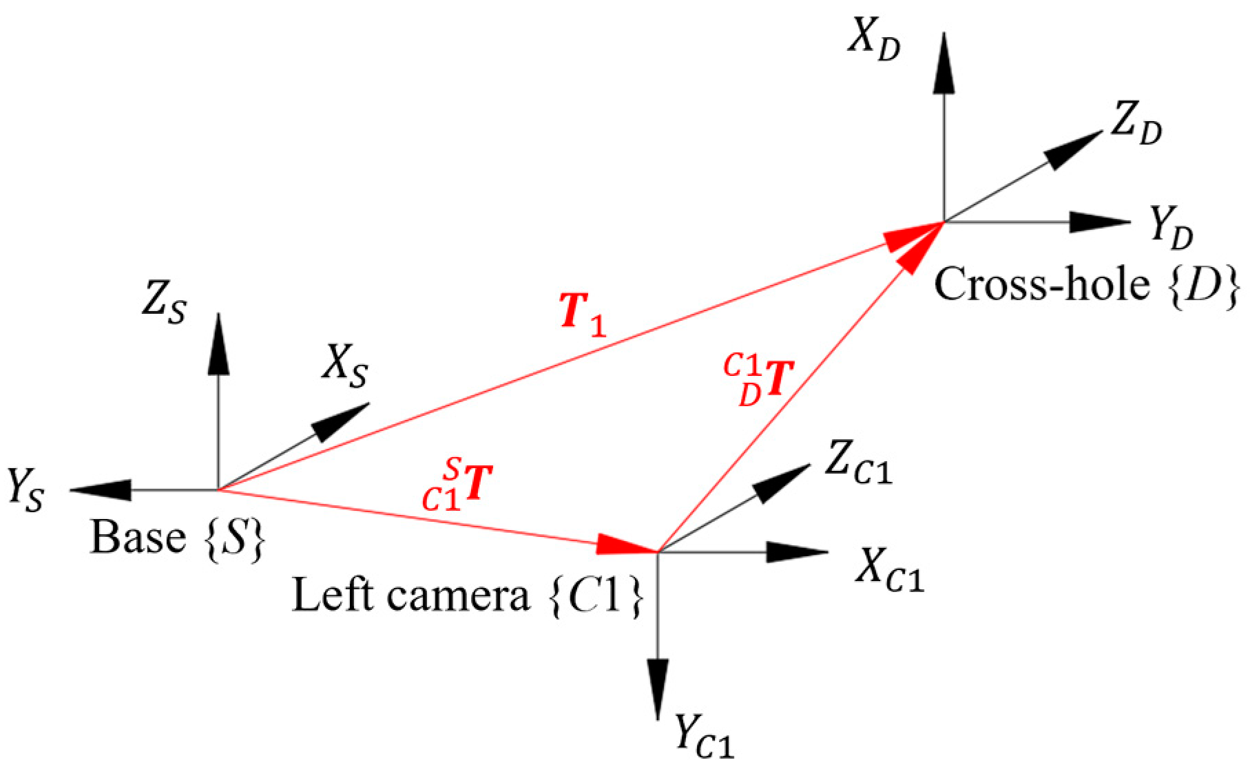
A schematic diagram of the coordinate and relative pose of the binocular vision system is depicted in Figure 5. The initial pose ${\mathit{T}}_1$ of the cross-hole coordinate system can be derived from the poses ${}_{C1}{}^S\mathit{T}$ and ${}_D{}^{C1}\mathit{T}$, which respectively represent the left camera coordinate system {C1}, with respect to the base coordinate system {S}, and the cross-hole coordinate system {D}, with respect to the left camera coordinate system {C1}.

The poses ${}_{C1}{}^S\mathit{T}$ of the left camera coordinate system {C1} with respect to the robot base coordinate system {S} are

$${}_{C1}{}^S\mathit{T}=\left(\begin{array}{cccc}0& 0& 1& p_x\\ -1& 0& 0& p_y\\ 0& -1& 0& p_z\\ 0& 0& 0& 1\end{array}\right)$$

(5)

where $p_x$, $p_y$, $p_z$ is the position of the camera coordinate system {C1} relative to the base coordinate system {S}.

The pose ${}^{C1}\mathit{T}_D$ of the cross hole coordinate system {D} with respect to the left camera coordinate system {C1} is

$${}^{C1}\mathit{T}_D=\left(\begin{array}{cccc}0& 1& 0& x_{C1}\\ -1& 0& 0& y_{C1}\\ 0& 0& 1& z_{C1}\\ 0& 0& 0& 1\end{array}\right)$$

(6)

where $x_{C1}$, $y_{C1}$, $z_{C1}$ is the position of the cross-hole center in the left camera coordinate system {C1}.

Then the pose ${\mathit{T}}_1$ of the coordinate system {D} under the coordinate system {S} of the robot arm base is

$${\mathit{T}}_1={}_{C1}{}^S\mathit{T}\cdot {}^{C1}\mathit{T}_D=\left(\begin{array}{cccc}0& 0& 1& p_x+z_{C1}\\ 0& -1& 0& p_y-x_{C1}\\ 1& 0& 0& p_z-y_{C1}\\ 0& 0& 0& 1\end{array}\right)$$

(7)

Using the 3D reconstruction principle of binocular vision, the three-dimensional coordinates $(x_{C1},y_{C1},z_{C1})$ of the center of the cross-hole in the left camera coordinate system {C1} are calculated as (0.0507, 0.0085, 0.3002), in meters. The transformation matrix ${}_{C1}{}^S\mathit{T}$ of the left camera coordinate system {C1} with respect to the base coordinate system {S} can be determined as

$${}_{C1}{}^S\mathit{T}=\left(\begin{array}{cccc}0& 0& 1& 0.1310\\ -1& 0& 0& -0.2406\\ 0& -1& 0& 0.2225\\ 0& 0& 0& 1\end{array}\right)$$

(8)

Substituting (8) into (7), the target pose ${\mathit{T}}_1$ of the cross-peg is obtained as

$${\mathit{T}}_1=\left(\begin{array}{cccc}0& 0& 1& 0.4312\\ -1& 0& 0& -0.2913\\ 0& -1& 0& 0.2140\\ 0& 0& 0& 1\end{array}\right)$$

(9)

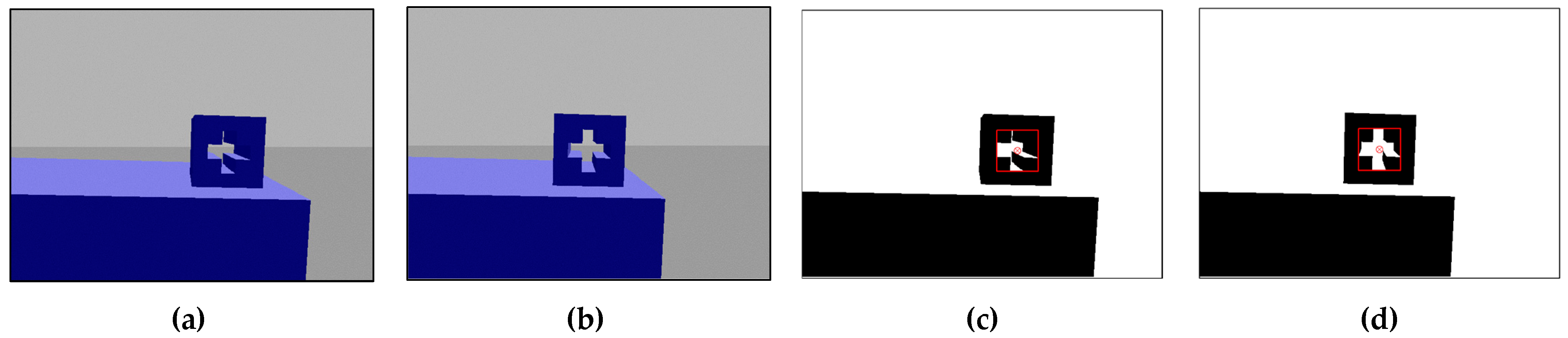
The images captured by the binocular camera in the simulation system are presented in Figure 6a, while Figure 6b displays the image obtained after image processing. The area enclosed by the red rectangle represents the cross-hole region, with its center marked by a red dot. In the left camera, the pixel coordinates of this center are (385, 253), while in the right camera they are (321.5, 252.5). The distance between both cameras’ optical axes is 0.05 m.

2.3. 6R Robot Trajectory Planning

To achieve the initial positioning and movement of the PiH task, it is necessary to plan the trajectory of the 6R robot so that it can move to position ${\mathit{T}}_1$. To ensure the smoothness of velocity and acceleration, a fifth-order polynomial is employed for interpolation [37], with $q_t$ representing the joint position of the robot at time t.

The position, velocity and acceleration of the interpolation starting point A are $q_0$, ${\dot{q}}_0$, and ${\ddot{q}}_0$, respectively, and the position, velocity, and acceleration of the interpolation target destination B are $q_T$, ${\dot{q}}_T$, and ${\ddot{q}}_T$, respectively. The time duration between point A and point B is denoted as T, which commences from the initial position A at $t=0$ and terminates at the destination B at t = T. Consequently, we can derive

$$\left\{\begin{array}{l}{q}_0=a_0\\ {\dot{q}}_0=a_1\\ {\ddot{q}}_0=2a_2\\ q_T=a_0+a_{1}T+a_2{T}^2+a_3{T}^3+a_4{T}^4+a_5{T}^5\\ {\dot{q}}_T=a_1+2a_{2}T+3a_3{T}^2+4a_4{T}^3+5a_5{T}^4\\ {\ddot{q}}_T=2a_2+6a_{3}T+12a_4{T}^4+20a_5{T}^3\end{array}\right.$$

(10)

The solution gives

$$\left\{\begin{array}{l}{a}_0=q_0\\ a_1={\dot{q}}_0\\ a_2={\displaystyle \frac{1}{2}}{\ddot{q}}_0\\ a_3={\displaystyle \frac{1}{2T^3}}\left[20\left(q_T-q_0\right)-\left(8{\dot{q}}_T+12{\dot{q}}_0\right)T+\left({\ddot{q}}_T-3{\ddot{q}}_0\right)T^2\right]\\ a_4={\displaystyle \frac{1}{2T^4}}\left[-30\left(q_T-q_0\right)+\left(14{\dot{q}}_T+16{\dot{q}}_0\right)T-\left(2{\ddot{q}}_T-3{\ddot{q}}_0\right)T^2\right]\\ a_5={\displaystyle \frac{1}{2T^5}}\left[12\left(q_T-q_0\right)-\left(6{\dot{q}}_T+6{\dot{q}}_0\right)T+\left({\ddot{q}}_T-{\ddot{q}}_0\right)T^2\right]\end{array}\right.$$

(11)

The coefficients can be obtained by inputting the initial joint angle and target joint angle into Equation (11), which are then substituted in $q_t$ to determine the joint angle of the robot arm at each time step. This information is transmitted to the robot for precise control over its movement, allowing it to reach the specified position ${\mathit{T}}_1$ and complete initial positioning of the PiH task.

The target joint angle ${q_T}^{\prime }$ is

$${q_T}^{\prime }=\left(-0.7143,1.1622,-0.0759,0.7751,-1.2112,-1.9028\right)$$

(12)

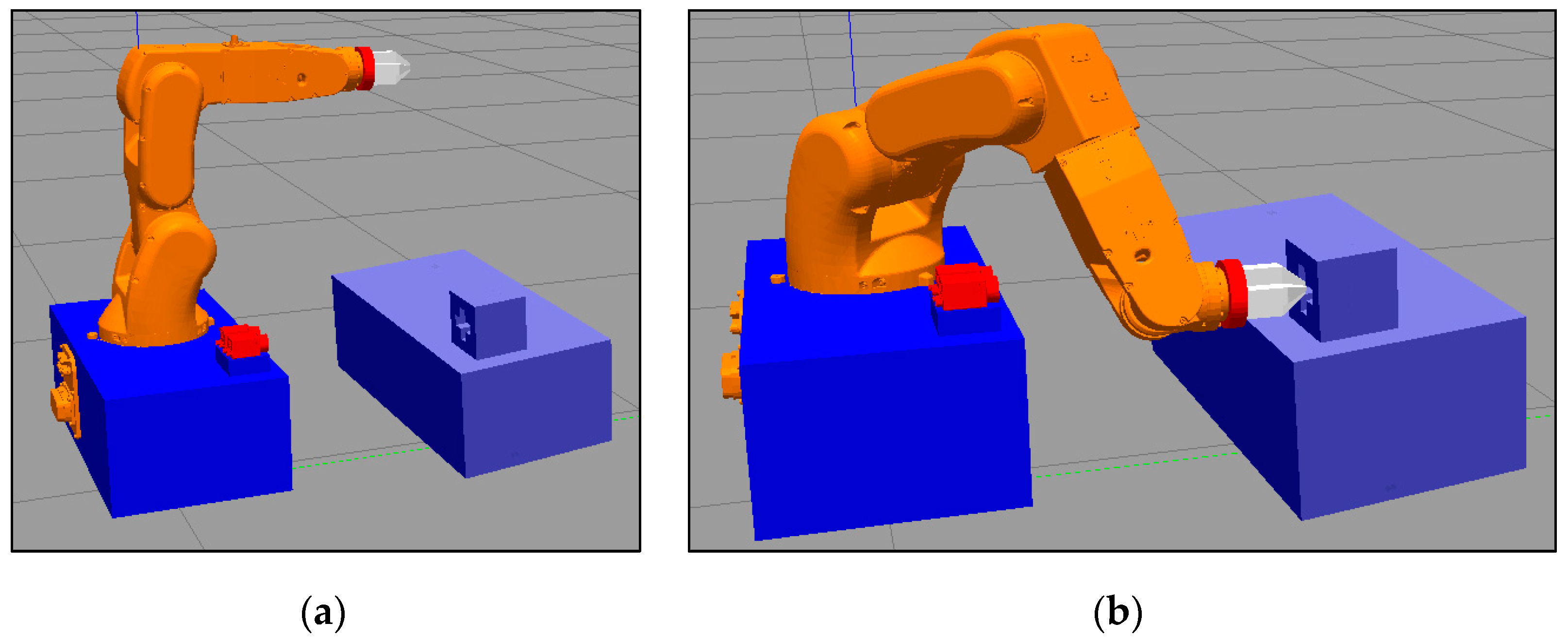
Figure 7a shows the initial pose of the 6R robot. As measured by ROS, in the initial state, the pose relationship between the cross-hole coordinate system {D} and the robot base coordinate system {S} is ${\mathit{T}}_0$, which is recorded for subsequent verification:

$${\mathit{T}}_0=\left(\begin{array}{cccc}-0.07& 0.06& 1& 0.4\\ -0.06& -1& 0.06& -0.3\\ 1& -0.06& 0.07& 0.2\\ 0& 0& 0& 1\end{array}\right)$$

(13)

After the interpolation trajectory planning of the 6R robot, Figure 7b depicts the robot’s attitude subsequent to its relocation to the designated position ${\mathit{T}}_1$. At this point, the axes of both cross-peg and cross-hole are collinear, but do not make contact. This marks the completion of the initial pose adjustment for the PiH task.

3. Force-Moment Sensor-Based Cross-Peg Insertion

After completing the initial positioning through a hole-searching process, the cross-peg can be inserted into the cross-hole by continuously adjusting its position according to the force-moment sensor value until the PiH task is completed. In this section, the force-moment sensor will be calibrated and gravity compensation will be implemented to mitigate the impact of inherent errors and external loads on the sensor’s measurements. Subsequently, the contact state of the peg and hole is classified and the mechanics of the assembly process are analyzed. Finally, a BP neural network mapping relationship between sensor data and assembly error is established to enable the independent assembly of the cross-peg.

3.1. Force-Moment Sensor Calibration and Gravity Compensation

The measured data of the force-moment sensor consists of three components: the inherent error of the sensor, the gravity acting on both the sensor and peg, and the external contact force applied to the feedback peg [38,39]. The gravity of the sensor and peg is denoted as G, and has its centroid located at $({}^{K}x,{}^{K}y,{}^{K}z)$ in coordinate system {D}. Based on the material and structural design, the gravity acting upon the force-moment sensor and cross-peg is 9.558 N.

The user has the flexibility to adjust the data in accordance with their own study. The value of the force-moment sensor at no load ${\mathit{F}}_0$, the measured value of the force-moment sensor ${\mathit{F}}_s$, and the contact force of the cross-peg ${\mathit{F}}_e$ can be recorded as

$$\left\{\begin{array}{l}{\mathit{F}}_0=\left(F_{x0},F_{y0},F_{z0},M_{x0},M_{y0},M_{z0}\right)\\ {\mathit{F}}_s=\left(F_x,F_y,F_z,M_x,M_y,M_z\right)\\ {\mathit{F}}_e=\left(F_{ex},F_{ey},F_{ez},M_{ex},M_{ey},M_{ez}\right)\end{array}\right.$$

(14)

According to the theory of least squares [40], it is obtained that

$$\mathit{m}=\left(\begin{array}{c}{M}_x\\ M_y\\ M_z\end{array}\right)=\left(\begin{array}{cccccc}0& F_z& -F_y& 1& 0& 0\\ -F_z& 0& F_x& 0& 1& 0\\ F_y& -F_x& 0& 0& 0& 1\end{array}\right)\left(\begin{array}{c}{}^{K}x\\ {}^{K}y\\ {}^{K}z\\ k_1\\ k_2\\ k_3\end{array}\right)=\mathit{F}\cdot \mathit{p}$$

(15)

where $k_1$, $k_2$, $k_3$ are the constants containing the force under no load, moment, and centroid coordinates.

To solve the matrix using least squares theory, it is necessary to guide the end joint of the robot through six distinct poses while ensuring that at least three of these poses have non-coplanar end-pointing vectors. Additionally, force-moment sensor data must be recorded for each pose.

Table 1. Force-moment sensor data in six poses.

No.	6R Robot Pose	Force (N)	Moment (Nm)
1	$\left(\begin{array}{rrrr}\hfill 0.0207& \hfill 0.0000& \hfill 0.9998& \hfill 0.5423\\ \hfill 0.0000& \hfill -1.0000& \hfill 0.0000& \hfill 0.0015\\ \hfill 0.9998& \hfill 0.0000& \hfill -0.0207& \hfill 0.6277\\ \hfill 0& \hfill 0& \hfill 0& \hfill 1\end{array}\right)$	$\begin{array}{c}-9.552\\ 0\\ 0\end{array}$	$\begin{array}{c}0\\ -0.308\\ 0\end{array}$
2	$\left(\begin{array}{rrrr}\hfill 0.9999& \hfill 0.0000& \hfill -0.0155& \hfill 0.3187\\ \hfill 0.0000& \hfill -1.0000& \hfill 0.0000& \hfill 0.0015\\ \hfill -0.0155& \hfill 0.0000& \hfill -0.9999& \hfill 0.4142\\ \hfill 0& \hfill 0& \hfill 0& \hfill 1\end{array}\right)$	$\begin{array}{c}0\\ -0.001\\ 9.552\end{array}$	$\begin{array}{c}0\\ -0.001\\ 0\end{array}$
3	$\left(\begin{array}{rrrr}\hfill 0.9999& \hfill -0.0148& \hfill 0.0000& \hfill 0.3219\\ \hfill 0.0000& \hfill 0.0000& \hfill 1.0000& \hfill 0.2193\\ \hfill -0.0148& \hfill -0.9999& \hfill 0.0000& \hfill 0.6356\\ \hfill 0& \hfill 0& \hfill 0& \hfill 1\end{array}\right)$	$\begin{array}{c}0.085\\ 9.553\\ 0\end{array}$	$\begin{array}{c}-0.308\\ 0.006\\ 0\end{array}$
4	$\left(\begin{array}{rrrr}\hfill 0.4114& \hfill 0.1916& \hfill 0.8911& \hfill 0.5707\\ \hfill 0.4007& \hfill -0.9161& \hfill 0.0120& \hfill 0.0484\\ \hfill 0.8187& \hfill 0.3521& \hfill -0.4537& \hfill 0.4670\\ \hfill 0& \hfill 0& \hfill 0& \hfill 1\end{array}\right)$	$\begin{array}{c}-7.802\\ -3.319\\ 3.955\end{array}$	$\begin{array}{c}0.124\\ -0.244\\ 0\end{array}$
5	$\left(\begin{array}{rrrr}\hfill 0.4922& \hfill 0.2466& \hfill 0.8348& \hfill 0.5616\\ \hfill 0.3714& \hfill -0.9269& \hfill 0.0548& \hfill 0.0590\\ \hfill 0.7873& \hfill 0.2830& \hfill -0.5478& \hfill 0.4038\\ \hfill 0& \hfill 0& \hfill 0& \hfill 1\end{array}\right)$	$\begin{array}{c}-7.695\\ -2.747\\ 4.947\end{array}$	$\begin{array}{c}0.0989\\ -0.244\\ 0\end{array}$
6	$\left(\begin{array}{rrrr}\hfill -0.1457& \hfill -0.1829& \hfill 0.9723& \hfill 0.6339\\ \hfill -0.2244& \hfill -0.9510& \hfill -0.2125& \hfill -0.1749\\ \hfill 0.9635& \hfill -0.2492& \hfill 0.0975& \hfill 0.5851\\ \hfill 0& \hfill 0& \hfill 0& \hfill 1\end{array}\right)$	$\begin{array}{c}-8.739\\ 2.220\\ -1.387\end{array}$	$\begin{array}{c}-0.104\\ -0.272\\ 0\end{array}$

shows the force-moment sensor data in six different poses.

The least squares solution p of the matrix from the force-moment sensor data is

$$\begin{array}{ll}\mathit{p}& ={\left({\mathit{F}}^{\mathrm{T}}\mathit{F}\right)}^{-1}\cdot {\mathit{F}}^{\mathrm{T}}\mathit{m}\\ & ={\left({}^{K}x,{}^{K}y,{}^{K}z,k_1,k_2,k_3\right)}^{\mathrm{T}}\\ & ={\left(0.0006,0.0011,0.0327,-0.0034,0.0081,-0.0065\right)}^{\mathrm{T}}\end{array}$$

(16)

Similarly, the results of the force-moment sensor calibrated by the least squares method are as follows:

$$\begin{array}{ll}{\mathit{F}}_0& =\left(F_{x0},F_{y0},F_{z0},M_{x0},M_{y0},M_{z0}\right)\\ & =\left(0.1714,-0.0426,-0.0153,-0.0020,0.0138,-0.0067\right)\end{array}$$

(17)

3.2. Peg-in-Hole Contact State Classification

The contact point of the PiH task is located at the intersection of the tapered end of the front guide section of the cross-peg and the edge line of the cross-hole, as shown in Figure 8.

Based on the advantages of the central symmetry cross-shaped peg and hole, two classification methods are proposed for categorizing contact states in the PiH insertion task: classification by the number of contact points and the rotation error of the cross-peg.

3.2.1. Classification by the Number of Contact Points

As shown in Figure 9, during the insertion of a cross-shaped peg, there are four types of contact states according to the number of contact points: one-point contact, two-point contact, three-point contact, and four-point contact.

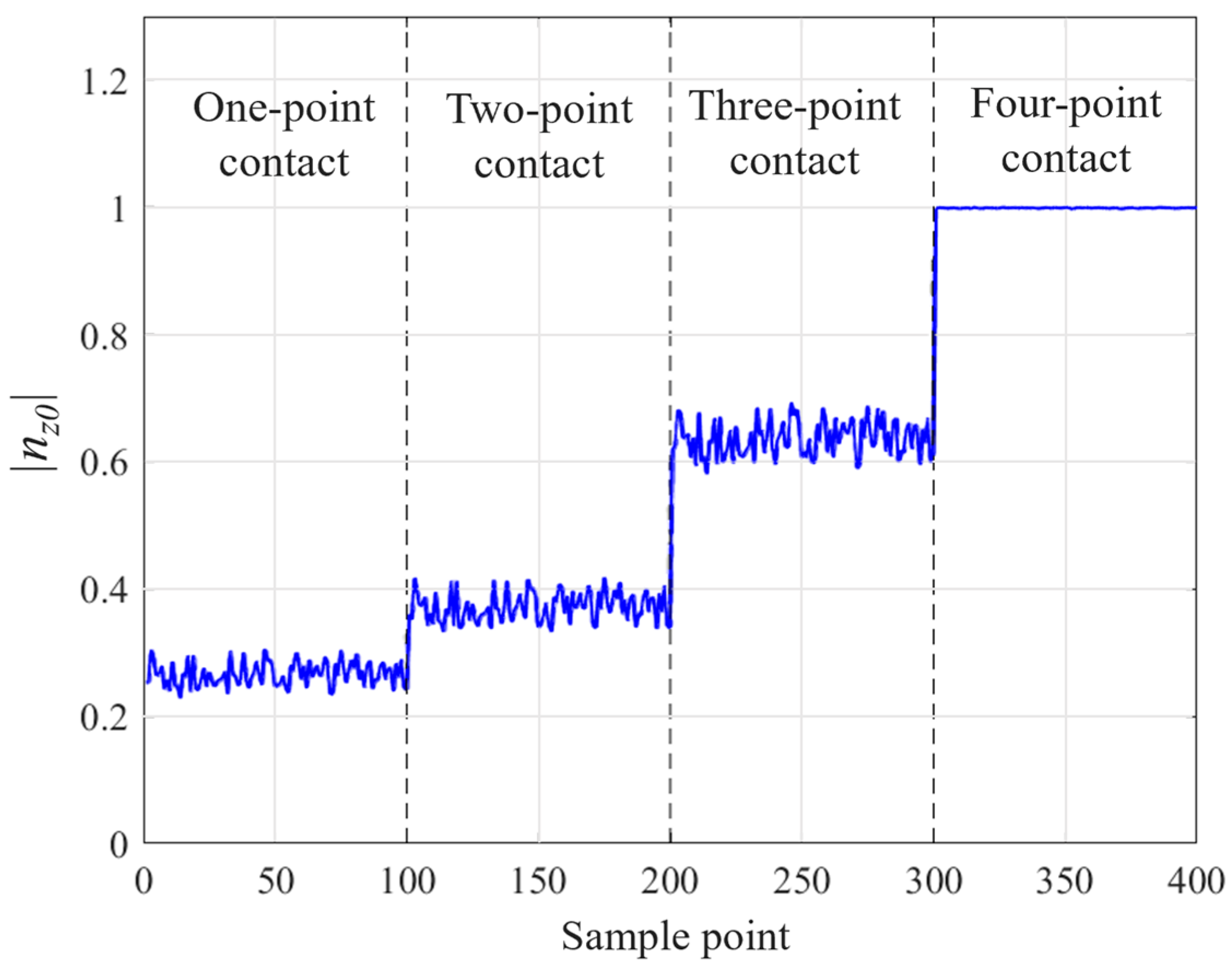
In Figure 9, it can be seen that the cross-peg circumferential forces and moments are more complex when the guide area of the cross-peg is in contact with the cross-hole, while the radial forces $F_{ez}$ are simpler and may be related to the number of contact points. To verify this hypothesis, the robot was manipulated to create 100 contacts between the cross-axis and cross-hole in one-point, two-point, three-point, and four-point states. The unit vector of the external force on the cross-peg is as follows:

$${\mathit{n}}_0=\left(\begin{array}{c}{n}_{x0}\\ n_{y0}\\ n_{z0}\end{array}\right)={\displaystyle \frac{1}{\sqrt{F_{ex}^2+F_{ey}^2+F_{ez}^2}}}\left(\begin{array}{c}{F}_{ex}\\ F_{ey}\\ F_{ez}\end{array}\right)$$

(18)

where the data of $\left|n_{z0}\right|$ are shown in Figure 10.

It can be seen in Figure 10 that $\left|n_{z0}\right|$ has a clear mapping relationship with the contact state; it is concluded that $\left|n_{z0}\right|$ is distributed between 0.23 and 0.31 with a mean value of 0.278 in the case of one-point contact, between 0.33 and 0.42 with a mean value of 0.376 in the case of two-point contact, between 0.58 and 0.71 with a mean value of 0.649 in the case of three-point contact, and is infinitely close to 1 in the case of four-point contact. According to the mapping relationship between $\left|n_{z0}\right|$ and the contact state, the contact state of the peg can be determined for subsequent inserting operations.

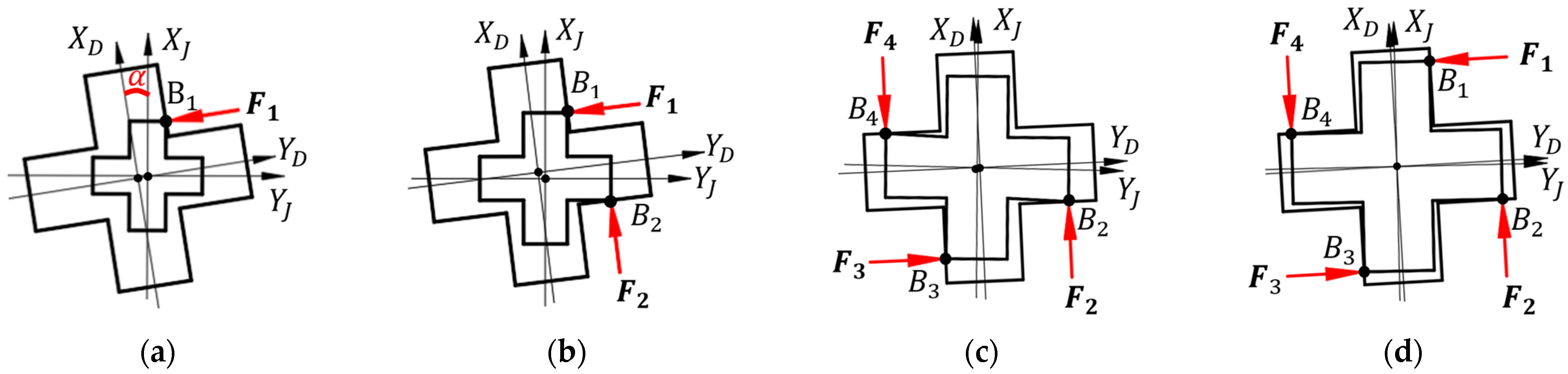
3.2.2. Classification by Rotation Error

The rotation angle of the cross-hole coordinate system {D} relative to the $Z_J$ axis of the cross-peg coordinate system {D} is α. Depending on the direction of rotation, it can be divided into the cases of $\alpha <0$ and $\alpha >0$, and Figure 11 shows the diagrams of the two different contact states.

3.3. Force-Moment Sensor for Each Contact State

The two states can be distinguished according to the direction of $M_{ez}$ in the force-moment sensor data; when $\alpha <0$, $M_z$ is negative, and when $\alpha >0$, $M_{ez}$ is positive. By combining the two classification methods mentioned in Section 3.2.1 and Section 3.2.2, a total of 26 different contact cases were obtained. To succinctly describe each contact state, a numbering system is utilized to express the contact cases. The format for this numbering system is as follows:

$$w_1-w_2-w_3$$

where $w_1$ indicates the number of contact points, ranging from 1 to 4; $w_2$ indicates the direction of rotation—$w_2=1$ when $\alpha <0$ and $w_2=2$ when $\alpha >0$; $w_3$ indicates the contact case when $w_1$ and $w_2$ are identical. For example, case 1-2-3 represents the third contact case with one-point contact and $\alpha >0$.

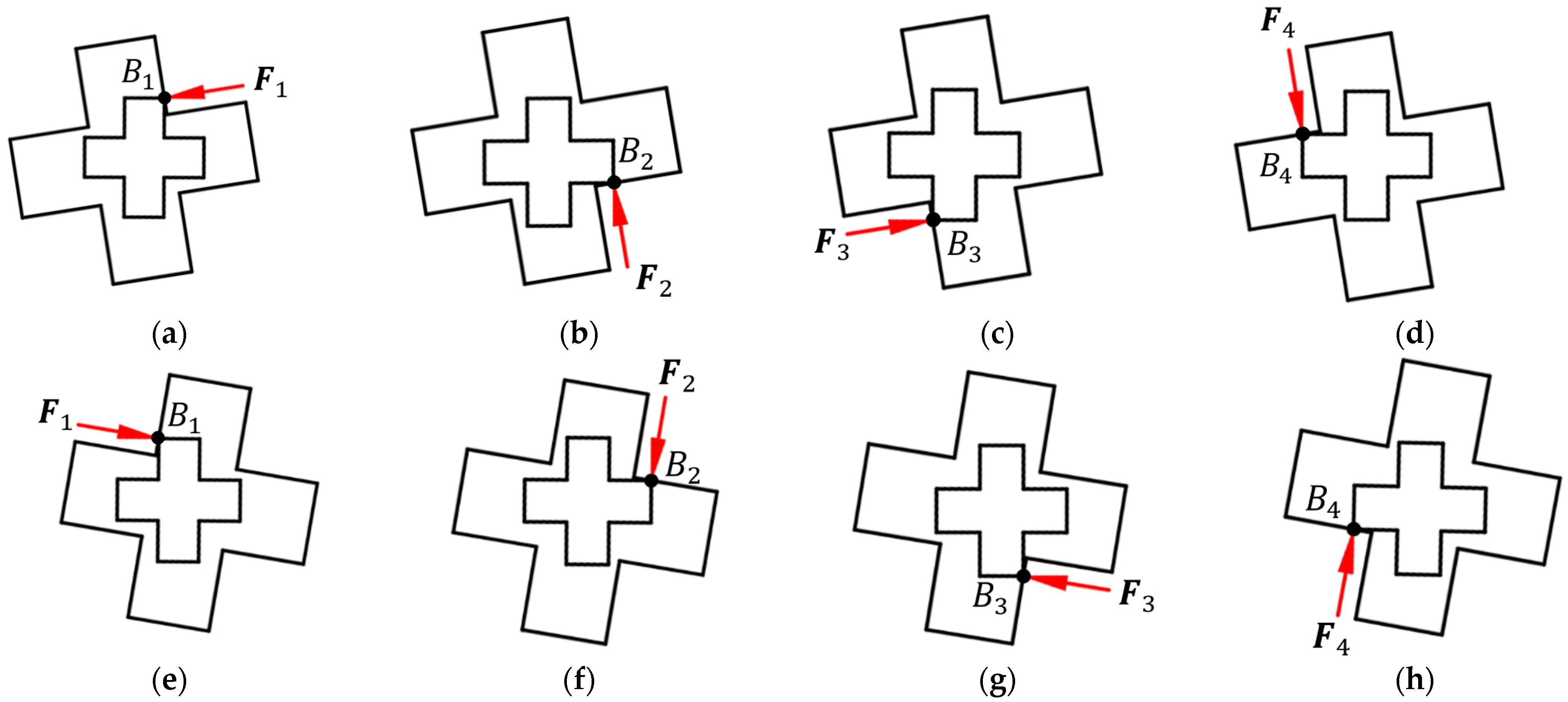
3.3.1. One-Point Contact

There are eight one-point contact cases, as shown in Figure 12. The force-moment sensor data for the one-point contact case is presented in

Table 2. Force-moment sensor value distribution of one-point contact cases.

Case	Fx	Fy	Fz	Mx	My	Mz
1-1-1	$\to$0	$-$	$-$	$+$	$\to$0	$-$
1-1-2	$+$	$\to$0	$-$	$\to$0	$+$	$-$
1-1-3	$\to$0	$+$	$-$	$-$	$\to$0	$-$
1-1-4	$-$	$\to$0	$-$	$\to$0	$-$	$-$
1-2-1	$\to$0	$+$	$-$	$-$	$\to$0	$+$
1-2-2	$-$	$\to$0	$-$	$\to$0	$-$	$+$
1-2-3	$\to$0	$-$	$-$	$+$	$\to$0	$+$
1-2-4	$+$	$\to$0	$-$	$\to$0	$+$	$+$

.

3.3.2. Two-Point Contact

There are eight two-point contact cases, as shown in Figure 13. The force-moment sensor data for the two-point contact case is presented in

Table 3. Force-moment sensor value distribution of two-point contact cases.

Case	Fx	Fy	Fz	Mx	My	Mz
2-1-1	$+$	$-$	$-$	$+$	$+$	$-$
2-1-2	$+$	$+$	$-$	$-$	$+$	$-$
2-1-3	$-$	$+$	$-$	$-$	$-$	$-$
2-1-4	$-$	$-$	$-$	$+$	$-$	$-$
2-2-1	$-$	$+$	$-$	$-$	$-$	$+$
2-2-2	$-$	$-$	$-$	$+$	$-$	$+$
2-2-3	$+$	$-$	$-$	$+$	$+$	$+$
2-2-4	$+$	$+$	$-$	$-$	$+$	$+$

.

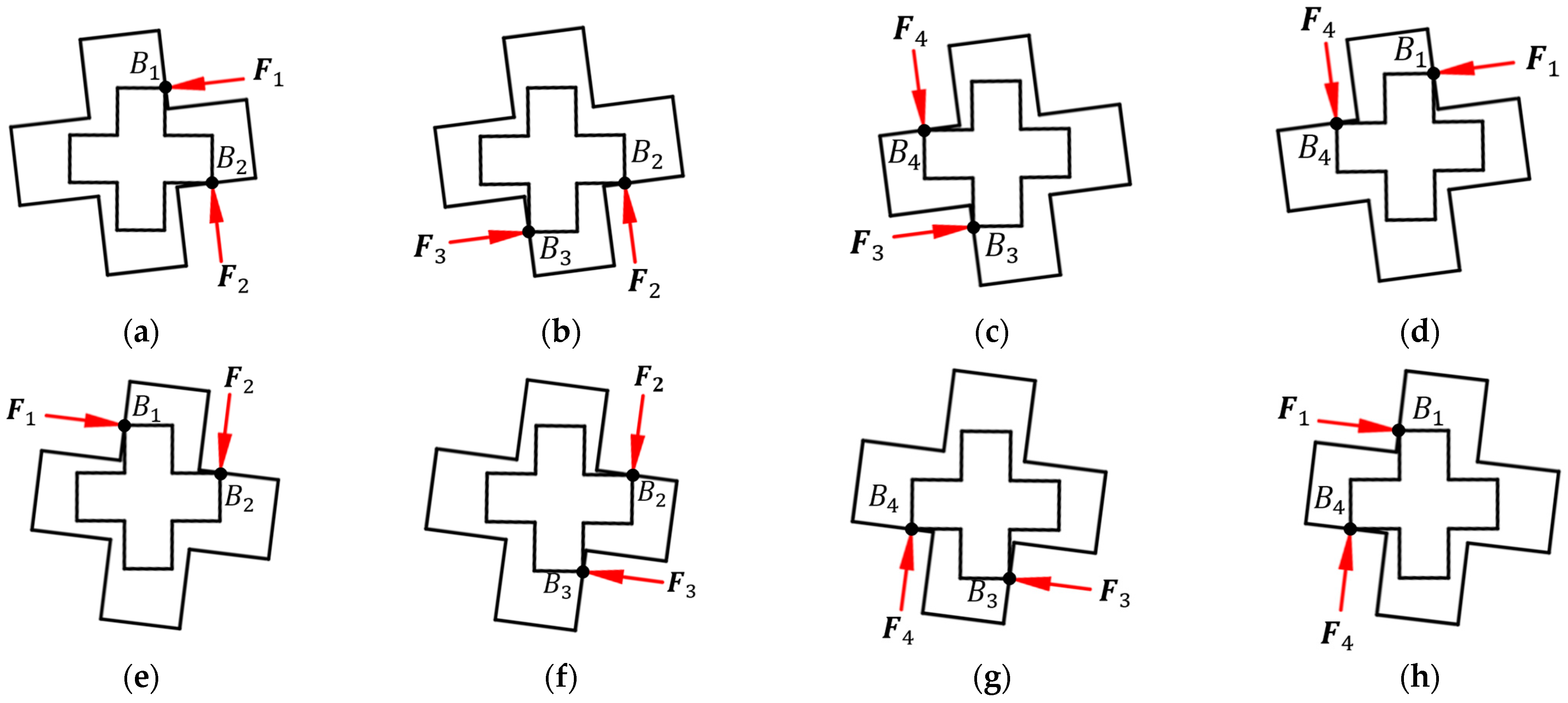
3.3.3. Three-Point Contact

There are eight three-point contact cases, as shown in Figure 14. The force-moment sensor data for the three-point contact case is presented in

Table 4. Force-moment sensor value distribution of three-point contact cases.

Case	Fx	Fy	Fz	Mx	My	Mz
3-1-1	$\to$0	$+$	$-$	$-$	$\to$0	$-$
3-1-2	$-$	$\to$0	$-$	$\to$0	$-$	$-$
3-1-3	$\to$0	$-$	$-$	$+$	$\to$0	$-$
3-1-4	$+$	$\to$0	$-$	$\to$0	$+$	$-$
3-2-1	$\to$0	$-$	$-$	$+$	$\to$0	$+$
3-2-2	$+$	$\to$0	$-$	$\to$0	$+$	$+$
3-2-3	$\to$0	$+$	$-$	$-$	$\to$0	$+$
3-2-4	$-$	$\to$0	$-$	$\to$0	$-$	$+$

.

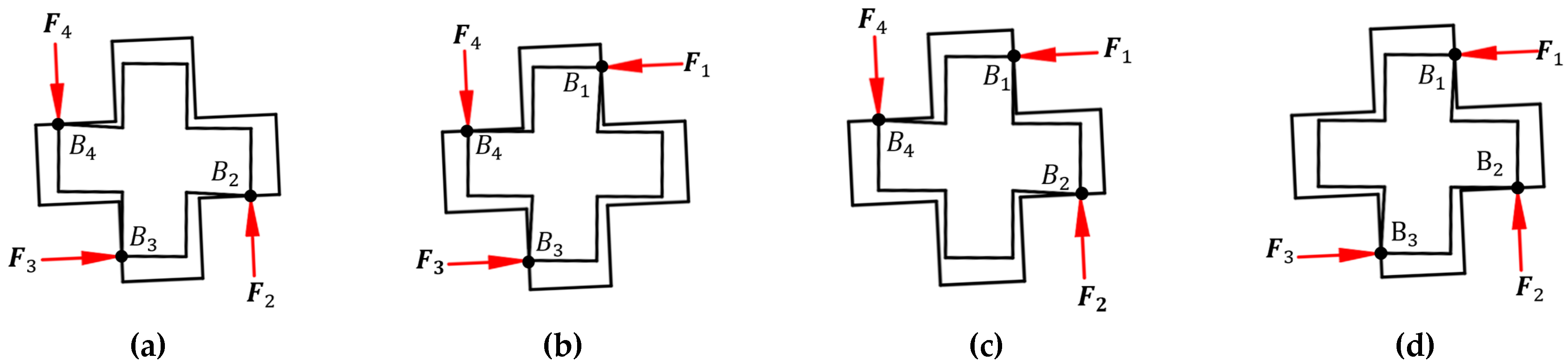
3.3.4. Four-Point Contact

There are two four-point contact cases, as shown in Figure 15. The force-moment sensor data for the four-point contact case is presented in

Table 5. Force-moment sensor value distribution of four-point contact cases.

Case	Fx	Fy	Fz	Mx	My	Mz
4-1-1	$\to$0	$\to$0	$-$	$\to$0	$\to$0	$-$
4-2-1	$\to$0	$\to$0	$-$	$\to$0	$\to$0	$+$

.

3.4. Mechanical Analysis of PiH Assembly

Figure 16 illustrates the force exerted when the cross-peg and cross-hole make contact with case 1-1-1. The contact point of the PiH task is located at the intersection of line $N_1{M}_1$ and line $D_1{D}_2$. The direction of the contact force F on the cross-peg is a normal vector of the plane formed by two lines, pointing to the inside of the cross-hole. The direction of the friction force $\mu F$ is along the tapered end of the cross-peg from point $M_1$ to point $N_1$.

The coordinates of the point $N_1$ are $\left(n_1,n_2,n_3\right)$, and the coordinates of the point $M_1$ are $\left(m_1,m_2,m_3\right)$. The coordinates of point $D_1$ and point $D_2$ in the cross-peg coordinate system {D} are $\left(x_1,y_1,z_1\right)$ and $\left(x_2,y_2,z_2\right)$, respectively. Then the coordinates of the contact point $B_1$ is

$$B_1=\left(\begin{array}{c}{B}_{1x}\\ B_{1y}\\ B_{1z}\end{array}\right)=\left(\begin{array}{c}{\displaystyle \frac{\frac{n_2-n_1}{m_2-m_1}\cdot \frac{x_2-x_1}{y_2-y_1}\cdot m_1+\left(n_1-y_1\right)\cdot \frac{x_2-x_1}{y_2-y_1}+x_1}{\frac{n_2-n_1}{m_2-m_1}\cdot \frac{x_2-x_1}{y_2-y_1}-1}}\\ \left(B_{1x}-x_1\right)\cdot {\displaystyle \frac{y_2-y_1}{x_2-x_1}}+y_1\\ \left(B_{1x}-x_1\right)\cdot {\displaystyle \frac{z_2-z_1}{x_2-x_1}}+z_1\end{array}\right)$$

(19)

The coordinates of each contact point in other contact cases can be solved using the same method, which will not be repeated in this paper.

The cross-peg is subjected to a contact force ${\mathit{F}}_1$ and a frictional force ${\mathit{f}}_1$ at the contact point $B_1$. The direction of the contact force ${\mathit{F}}_1$ is normal to the plane formed by line $N_1{M}_1$ and line $D_1{D}_2$, pointing inside the cross-peg; the direction of the frictional force ${\mathit{f}}_1$ is along line $N_1{M}_1$, opposite to the direction of movement of the cross-peg.

The direction vector of the contact force ${\mathit{F}}_1$ is

$${\mathit{n}}_1=\left(\begin{array}{c}{n}_{1x}\\ n_{1y}\\ n_{1z}\end{array}\right)={\displaystyle \frac{\overrightarrow{M_1{N}_1}\times \overrightarrow{D_1{D}_2}}{\left|\overrightarrow{M_1{N}_1}\times \overrightarrow{D_1{D}_2}\right|}}$$

(20)

Assuming the magnitude of the contact force on the cross-peg at the contact point $B_1$ is $F_1$, then

$${\mathit{F}}_1=\left(\begin{array}{c}{F}_{1x}\\ F_{1y}\\ F_{1z}\end{array}\right)=\left(\begin{array}{c}{F}_1\cdot n_{1x}\\ F_1\cdot n_{1y}\\ F_1\cdot n_{1z}\end{array}\right)=F_1\cdot {\mathit{n}}_1$$

(21)

Since the direction of the frictional force ${\mathit{n}}_{f1}$ is

$${\mathit{n}}_{f1}=\left(\begin{array}{c}{n}_{f1x}\\ n_{f1y}\\ n_{f1z}\end{array}\right)={\displaystyle \frac{\overrightarrow{M_1{N}_1}}{\left|\overrightarrow{M_1{N}_1}\right|}}$$

(22)

Then the frictional force ${\mathit{f}}_1$ is

$${\mathit{f}}_1=\left(\begin{array}{c}{f}_{1x}\\ f_{1y}\\ f_{1z}\end{array}\right)=\left(\begin{array}{c}\mu F_1\cdot n_{f1x}\\ \mu F_1\cdot n_{f1y}\\ \mu F_1\cdot n_{f1z}\end{array}\right)=\mu F_1\cdot {\mathit{n}}_{f1}$$

(23)

Additionally, the force-moment sensor value on the cross-peg is then

$$\left\{\begin{array}{l}{F}_{ex}={\displaystyle \sum _{i=1}^4\left(F_{ix}+f_{ix}\right)}\\ F_{ey}={\displaystyle \sum _{i=1}^4\left(F_{iy}+f_{iy}\right)}\\ F_{ez}={\displaystyle \sum _{i=1}^4\left(F_{iz}+f_{iz}\right)}\\ M_{ex}={\displaystyle \sum _{i=1}^4\left(-F_y\cdot B_{iz}+F_z\cdot B_{iy}\right)}\\ M_{ey}={\displaystyle \sum _{i=1}^4\left(F_x\cdot B_{iz}-F_z\cdot B_{ix}\right)}\\ M_{ez}={\displaystyle \sum _{i=1}^4\left(-F_x\cdot B_{iy}+F_y\cdot B_{ix}\right)}\end{array}\right.$$

(24)

where $i$ represents the contact point number for each contact state.

The relative error $\alpha ,\beta ,\gamma ,x,y,z$ between the peg and hole can be obtained by solving Equation (24) and then adjusting the peg pose according to the error.

4. Automatic PiH Assembly Based on BP Neural Network

4.1. Establishment of BP Neural Network

Due to the numerous unknowns and lengthy solution time of Equation (24), a mapping relationship between force-moment sensors and angle errors was established based on BP neural networks in order to achieve automatic assembly. [41]. This enables the robot to adjust its pose directly by obtaining the angular error from sensor data when the peg and hole are in contact, thereby realizing PiH tasks automatically.

The input layer consists of three force components and three moment components, which are measured by the force-moment sensor. The main purpose of establishing the BP neural network is to predict the angular error between the peg and the hole through force-moment sensor data, so the output layer consists of three angle error $\alpha$, $\beta$, $\gamma$ in three directions. The BP neural network algorithm places high demand on the network structure. Although increasing the number of network layers can reduce training errors, it also makes the BP neural network more complicated and increases training time. For the problem of mapping the relationship between sensor data and angle error, the BP neural networks with only one implicit layer can solve the problem, and the error can be reduced by increasing the number of neurons in the implicit layer. Therefore, a three-layer BP neural network model with only one hidden layer was used for this study.

The transfer function plays a crucial role in determining the error rate, computational complexity, and training efficiency of the BP neural network model. In this study, the evaluation index values were standardized to a range of 0 to 1, thus necessitating the selection of the Sigmoid function as the transfer function for the hidden layer. Due to the limited number of samples used in the PiH assembly process, the accuracy of the output results is impacted by the traditional BP neural network’s processing of a restricted sample size. Traingdx is specifically associated with the Matlab 2022b Neural Network Toolbox, a software package for designing, implementing, and simulating neural networks. Therefore, the traingdx function is used to shorten the time required to reach the specified accuracy to a certain extent, avoid the oscillation phenomenon in the training process, and improve the convergence speed and learning accuracy [42]. The BP neural network model established in this paper based on the above analysis is illustrated in Figure 17.

4.2. BP Neural Network Training Process

The BP neural network presented in this paper utilizes force-moment sensor data as the input and predicts angular error as the output. The sample data required for training are obtained through ROS, where the pose of the cross-peg is adjusted, and force-moment sensor data and angle error data are collected as samples for training in 26 states. This mapping relationship between sensor information and angle error allows the robot to autonomously determine its state and execute PiH tasks.

Table 6. Input training data of force-moment sensor values.

No.	Fx (N)	Fy (N)	Fz (N)	Mx (Nm)	My (Nm)	Mz (Nm)
1	−19.115	−0.949	−5.448	−0.031	−1.239	0.325
2	−19.833	−1.806	−6.285	−0.007	−1.226	0.375
3	−17.606	−0.126	−4.485	−0.088	−1.046	0.376
4	−20.706	−0.542	−5.556	−0.098	−1.161	0.266
5	−15.283	−1.343	−4.804	0.002	−0.977	0.481
6	−20.073	−0.809	−5.593	−0.063	−1.217	0.403
7	−19.654	−0.332	−5.145	0.101	−1.113	0.456
8	−19.699	−1.912	−6.341	−0.014	−1.177	0.399
9	−18.935	−0.707	−5.251	−0.067	−1.132	0.396
10	−19.154	−1.281	−5.717	−0.043	−1.130	0.398

and

Table 7. Output training data of angle errors.

No.	$\mathit{\alpha }$ (rad)	$\mathit{\beta }$ (rad)	$\mathit{\gamma }$ (rad)
1	0.07	0.07	0.07
2	0.1	0.04	0.03
3	0.02	0.1	0.05
4	0.04	0.06	0.05
5	0.1	0.1	0.04
6	0.06	0.05	0.07
7	0.03	0.01	0.05
8	0.1	0.01	0.01
9	0.04	0.09	0.01
10	0.07	0.03	0.01

display a portion of the training samples.

Due to the significant difference in size between the training data, normalization is necessary to facilitate effective training:

$$F_i={\displaystyle \frac{X_i-X_{\min }}{X_{i\max }-X_{i\min }}}$$

(25)

where $X_i$ is the No. $i$ sample data of the indicator obtained, $F_i$ is standardized value of $X_i$, $X_{i\max }$ is the maximum value in the No. $i$ sample data of the indicator obtained, and $X_{i\min }$ is the smallest value in the No. $i$ sample data of the indicator obtained.

Through continuous testing and evaluation, it was determined that the optimal performance is achieved when there are 150 neurons in the hidden layer. The logsig function is used for the input layer transfer function, while the pureline function is used for the hidden layer transfer function. These functions are part of the Matlab packages. The traingdx function is employed as the training function, with mean square error (MSE) serving as the performance function. The target error is 0.001, and the maximum number of iterations for learning is set to 1000.

Figure 18 shows the validation results after training, showing the sample values and test values, as well as the errors between them for each angle error. The errors are within 1°, which meet the requirements of PiH assembly [43]. Using this mapping model, the angular error can be swiftly and accurately obtained and substituted into Equation (24), while the translation error can be calculated in a short time.

5. Experiments

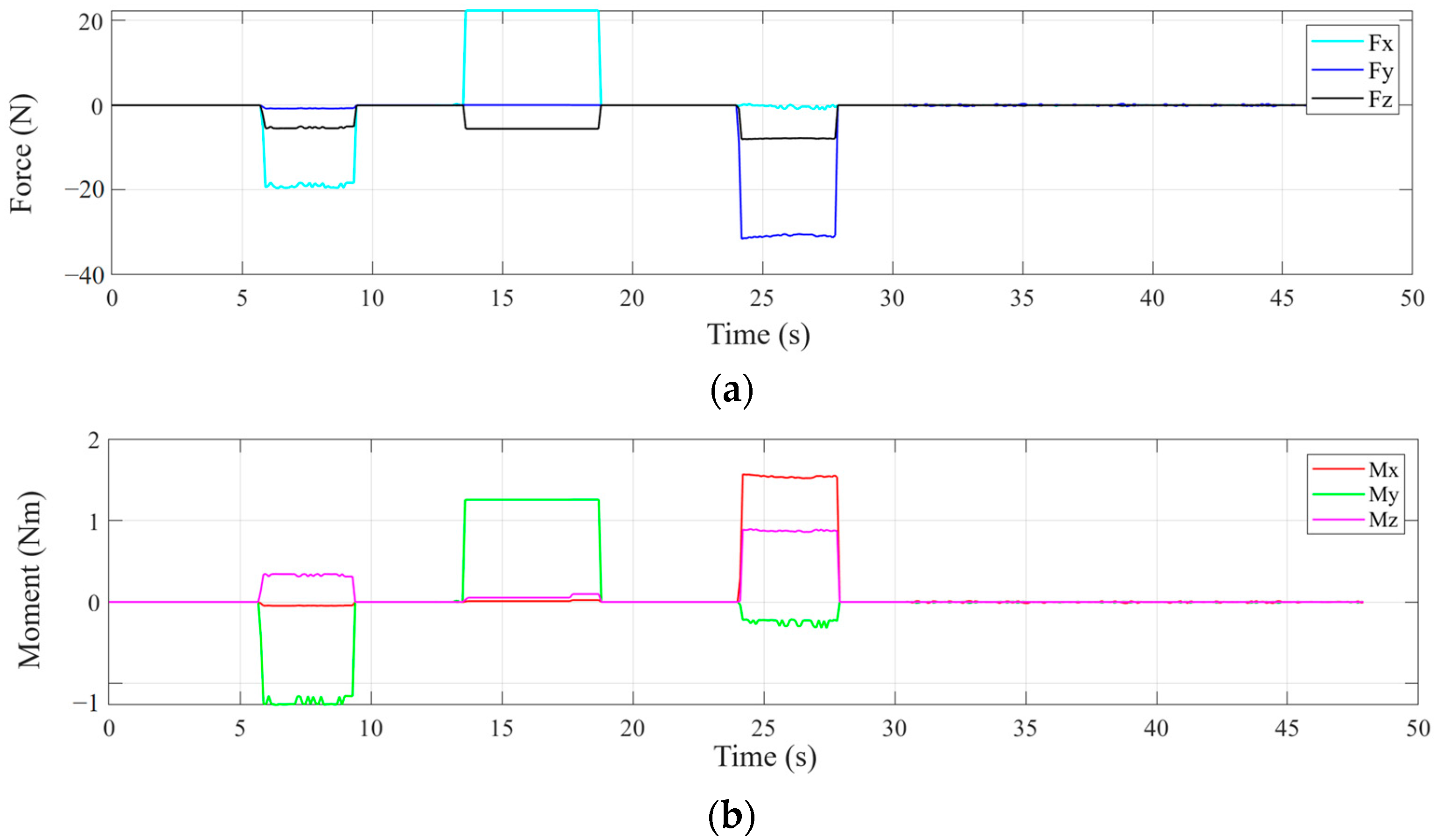
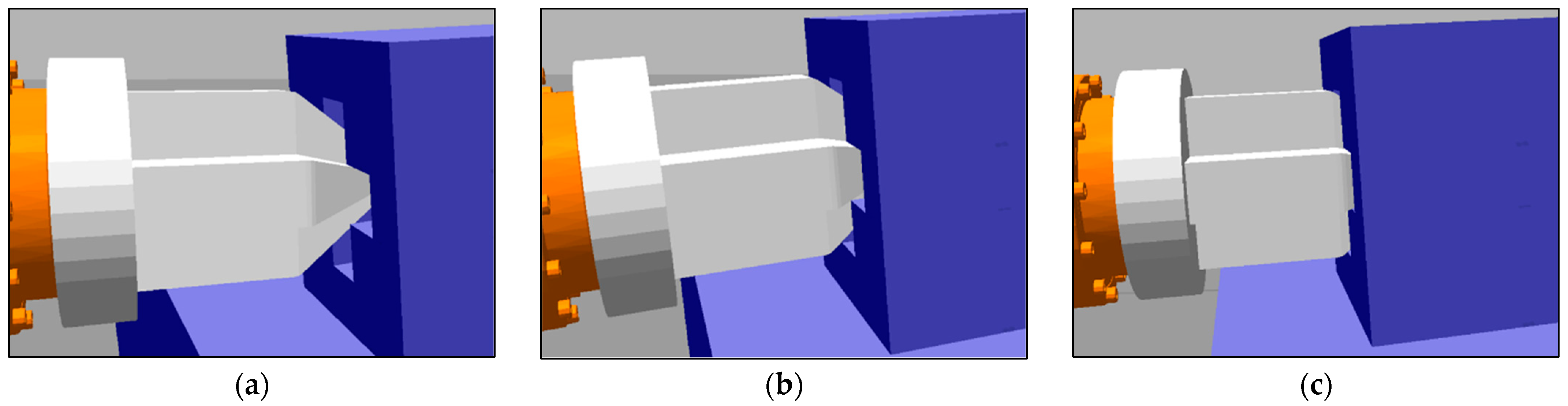
After completing the calibration of the force-moment sensor and BP neural network training, the assembly process of the cross-peg and cross-hole can be executed; the changes in the contact force and moment between the peg and the hole during the assembly process are shown in Figure 19.

At approximately 0 to 5 s, the cross-peg begins to move along its axis without any contact with the cross-hole, as shown in Figure 20a. The force-moment sensor reading value remains at zero. At around 6 s, the cross-peg continues to approach and insert into the cross-hole, resulting in an abrupt change in sensor value that indicates initial contact between the peg and the hole. The contact force value is (−19.247, −0.785, −5.3953) N, while the moment value is (−0.044, −1.244, 0.339) Nm.

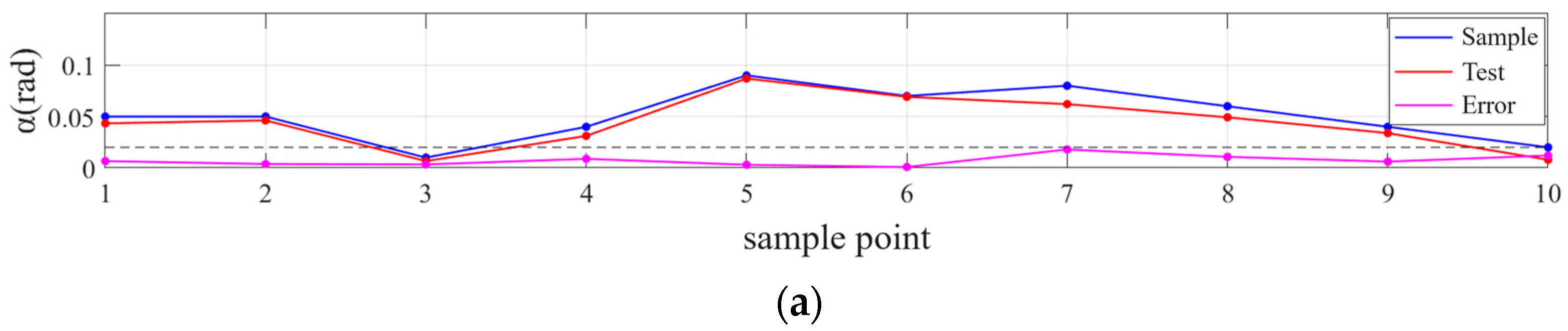
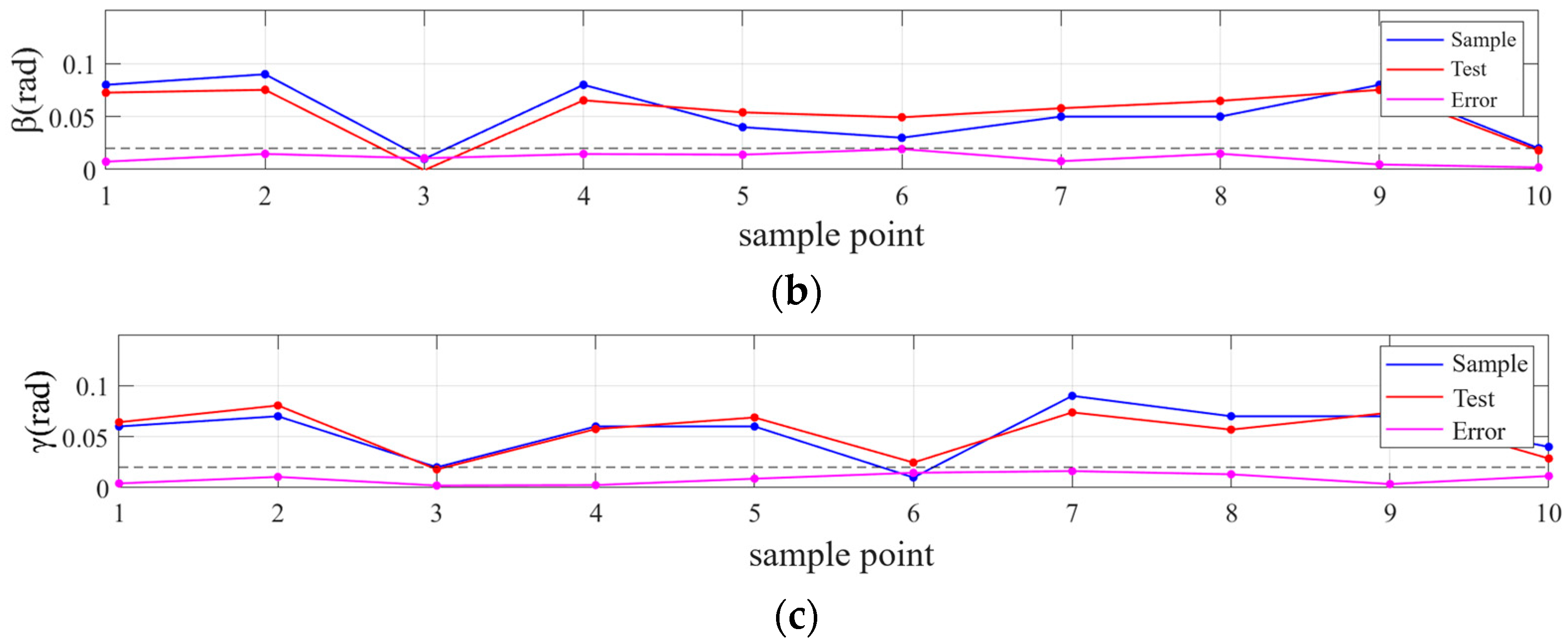
Using the established BP neural network, the contact state is judged to be 1-2-2, and the mapping relationship between force-moment sensor values and angle errors is obtained as (0.057, 0.074, 0.076) rad in the cross-hole coordinate system. The corresponding force-moment sensor values and angle errors are (−0.011, 0.006, 0.065) m. According to the calculated error, the robot pose is adjusted, the contact force between the peg and the hole is restored to zero after the adjustment, and the cross-peg continues to move along its axis. Similar to the above process, the second contact occurs around 13 s, as shown in Figure 20b, after automatic pose adjustment; the third contact occurs around 24 s, as shown in Figure 20c, and the assembly is completed after 27 s.

After the third adjustment is completed, the force-moment sensor data is close to 0 due to the frictional force existing in the peg. The increase in cross-peg insertion depth no longer generates abrupt changes, indicating that the relative error between the peg and the hole has been adjusted within acceptable accuracy limits. The state of the system after completion of PiH assembly is shown in Figure 21, wherein the cross-peg coordinate system {D} coincides with the cross-hole coordinate system {D}, and the position of each joint angle of the robot arm is

$$\mathit{\theta }=\left(-0.7692,1.1936,-0.1269,0.8692,-1.3075,-0.4335\right)$$

The joint angle is substituted into the transformation matrix of the robot link to obtain the relative pose ${\mathit{T}}_2$ of the cross-hole coordinate system {D} relative to the robot base coordinate system {S}, which is

$${\mathit{T}}_2=\left(\begin{array}{cccc}-0.0690& 0.0745& 0.9948& 0.4365\\ -0.0594& -0.9957& 0.0704& -0.3139\\ 0.9959& -0.0542& 0.0731& 0.2042\\ 0& 0& 0& 1\end{array}\right)$$

The relative pose obtained by the autonomous assembly system exhibits a negligible error relative to the pose measured by ROS in the initial state as shown in Equation (13), thereby validating the accuracy and correctness of the autonomous assembly system.

6. Conclusions

Based on the limitations of current peg-in-hole assembly, which mostly involves circular pegs and holes, and the fact that rotational DoF cannot be restricted about their axes after circular hole assembly, resulting in difficulty in obtaining the precise relative pose between the robot base and the hole, this paper proposes a new PiH assembly strategy by designing a cross-shaped peg and hole.

As many studies have focused solely on the insertion of pegs in PiH tasks, this paper aimed to establish a comprehensive autonomous assembly system that includes hole-searching and insertion based on force/moment and visual information. Therefore, the central coordinates of the cross-hole were obtained based on the three-dimensional reconstruction theory of binocular stereo vision. The trajectory for the robot was planned to align the axis of the cross-peg with the cross-hole without physical contact, thus achieving an autonomous hole-searching process. Then, all 26 contact states of cross-peg and cross-hole were classified and numbered according to the number of contact points and angle errors between the peg and the hole, and the force-moment sensor value under different contact states was summarized; then, the BP neural network was trained based on the sensor information and the relative errors of the cross peg and cross holes to establish the mapping relationship between force and error. Then, the cross-peg and cross-hole contact states were classified and numbered based on the number of contact points and angle errors between them. The force-moment sensor values under different contact states were summarized, and a BP neural network was trained using this information with relative errors to establish a mapping relationship between force and error. Finally, the PiH task was successfully executed to address the autonomous assembly challenge of the cross-peg and cross-hole, thereby obtaining the relative pose between the robot base coordinate system and the cross-hole coordinate system.

This new assembly strategy can replace the use of cross-pegs and cross-holes once this pose is obtained, enabling the assembly of more complex-shaped PiH tasks, such as spline assembly and square peg assembly. This solves the problem in which users need to reformulate the assembly strategy or design special sensors according to the size and shape of the peg. This not only reduces users’ workload but also enhances industrial production efficiency.

However, the research on this topic still needs to be improved, and our future research directions are as follows:

• Firstly, to compare the assembly efficiency and convergence speed of the mapping model under different algorithms, such as reinforcement learning and iterative learning control;
• Secondly, the replacement of various shaped pegs and holes to test their assembly effects was not conducted in this article. However, future research will focus on this area;
• Finally, if the 6R robot can be fixed on a 6-DoF platform, after obtaining the relative pose of the robot base coordinate system and the cross-hole coordinate system, the platform can achieve rendezvous and docking with another platform while continuously detecting the docking process based on the follow-up function of the 6R robot. After the system is built, it can realize the assembly task of heavy machinery, such as rocket tank assembly and missile assembly.