Fault Detection in Harmonic Drive Using Multi-Sensor Data Fusion and Gravitational Search Algorithm

Abstract

This study proposes a fault diagnosis method for harmonic drive systems based on multi-sensor data fusion and the gravitational search algorithm (GSA). As a critical component in robotic arms, harmonic drives are prone to failures due to wear, less grease, or improper loading, which can compromise system stability and production efficiency. To enhance diagnostic accuracy, the research employs wavelet packet decomposition (WPD) and empirical mode decomposition (EMD) to extract multi-scale features from vibration signals. These features are subsequently fused, and GSA is used to optimize the high-dimensional fused features, eliminating redundant data and mitigating overfitting. The optimized features are then input into a support vector machine (SVM) for fault classification, with K-fold cross-validation used to assess the model’s generalization capabilities. Experimental results demonstrate that the proposed diagnosis method, which integrates multi-sensor data fusion with GSA optimization, significantly improves fault diagnosis accuracy compared to methods using single-sensor signals or unoptimized features. This improvement is particularly notable in multi-class fault scenarios. Additionally, GSA’s global search capability effectively addresses overfitting issues caused by high-dimensional data, resulting in a diagnostic model with greater reliability and accuracy across various fault conditions.

1. Introduction

With the rapid development of industrial automation and the ever-growing demand for efficiency [1], many companies have introduced robotic arms to achieve automated production, further accelerating the demand for these systems. In the fields of manufacturing and precision machining, the application of robotic arms has become increasingly vital, particularly in enhancing production efficiency, precision, and stability. At the core of these systems is the harmonic drive, a key component that enables the realization of such goals. Harmonic drives, known for their high reduction ratios, high torque, and precision, are widely used in various joints of robotic arms, playing a critical role in improving overall system performance. Their integration into robotic systems has significantly boosted the capabilities and reliability of automated processes in industries where accuracy and stability are paramount.

As mechanical equipment operates for extended periods, factors such as wear and tear or improper human operation gradually increase the risk of unexpected failures. Andrea et al. [2] summarized common failure types in rotating machinery, identifying issues such as improper loading, insufficient lubrication, gear wear, and tooth breakage. These failures not only reduce the operational efficiency of robotic arms but can also lead to financial losses during production and even cause severe industrial safety incidents. To improve the reliability and stability of rotating machinery, various novel fault diagnosis methods have been proposed in recent years [3,4]. Common fault detection techniques for rotating machinery include vibration analysis [5,6], current monitoring [7,8,9], noise detection [10], and temperature monitoring [11,12]. Currently, most existing research remains focused on using single-sensor signals, such as vibration or current signals, for fault diagnosis. While these methods have achieved some success in single-fault mode scenarios, the increasing complexity of mechanical systems has exposed the limitations of single-sensor approaches. Specifically, they struggle to fully capture the intricate features present in multiple fault modes, leading to a decline in diagnostic accuracy. To address this issue, multi-sensor signal fusion technologies [13,14] have recently been applied in the field of fault diagnosis, yielding significant advancements, particularly in detecting issues like bearing defects and insufficient lubrication [15,16,17,18]. Multi-sensor fusion can effectively enhance diagnostic accuracy and reliability, providing more comprehensive diagnostic information for mechanical fault detection. However, extracting useful fault-related features from these multi-source signals remains a critical challenge. To overcome this, various signal processing methods have been developed to extract key features from complex mechanical vibration signals. Common frequency-domain analysis methods, such as Fourier transform (FT) [19] and time-frequency analysis (TFA) [20] methods, including wavelet transform (WT) [21], wavelet packet decomposition (WPD), empirical mode decomposition (EMD) [22], empirical wavelet transform (EWT) [23], and discrete wavelet transform (DWT) [24], have been widely used in fault diagnosis for mechanical systems, demonstrating their efficacy in detecting defects in critical components like bearings [25,26] and gears [27]. Through these methods, potential faults in harmonic drives can be more accurately identified and predicted, enabling computation time condition monitoring (CM) and fault detection and diagnosis (FDD) for robotic arms [28,29]. Although multi-sensor fusion provides more dimensions of diagnostic information, it also poses several challenges in practical applications. First, the feature shape and scale inconsistency between different sensor signals may lead to imbalance issues during data fusion, potentially affecting model performance. Additionally, the increased number of features results in high-dimensional data, raising computational complexity. If the selected features during the fusion process fail to represent the fault modes accurately, noise could be introduced, thus reducing diagnostic accuracy. Therefore, choosing appropriate feature extraction methods is crucial for overcoming these challenges.

Therefore, WPD and EMD were selected for multi-level feature extraction from vibration signals, as both methods excel in handling non-stationary signals and can extract fault-related high-frequency and low-frequency features across different frequency domains [30,31,32]. To enhance diagnostic accuracy, we utilized the gravitational search algorithm (GSA) [33,34,35] to optimize the fused features, capitalizing on its distinct advantages for this application. GSA models the behavior of masses under gravitational attraction, where solutions with better fitness attract others, facilitating a rapid and effective convergence toward the global optimum. This process makes GSA particularly adept at handling high-dimensional and complex datasets, as it efficiently explores vast solution spaces without becoming trapped in local optima. Its capacity to dynamically adjust search parameters based on fitness ensures reliable feature optimization, making it a highly effective choice for enhancing diagnostic accuracy and computational efficiency in fault detection tasks [36,37]. Initially, WPD and EMD were used to extract multi-level features from vibration signals, followed by feature fusion, and the fused features were then optimized using GSA. The optimized features were input into a machine-learning model, significantly improving fault diagnosis accuracy [38,39]. This approach effectively addresses redundant features and feature inconsistency issues during the fusion process and demonstrates superior performance in fault diagnosis. The contributions of this paper are as follows:

• The proposed method integrates feature fusion with GSA optimization. By fusing decomposed features and applying optimization, we demonstrate through experiments that the method effectively reduces overfitting in high-dimensional data. Furthermore, by optimizing feature selection, it eliminates the interference of redundant features, significantly improving diagnostic accuracy across multiple fault modes.
• Multi-sensor vibration data of harmonic drives were collected under various operating conditions. It was verified that the diagnostic model, after feature fusion and GSA optimization, achieved significantly higher accuracy compared to models using only data fusion.
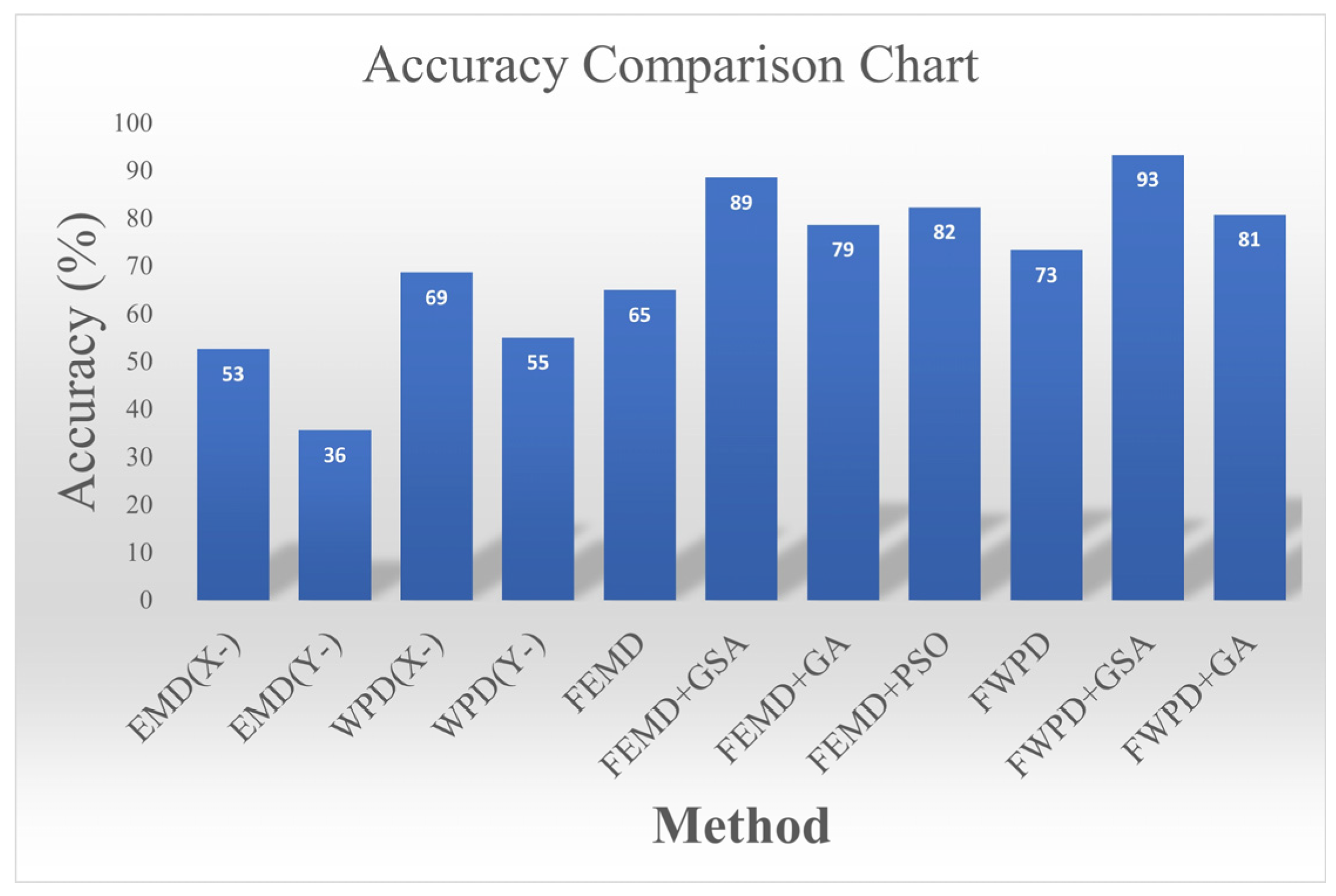
• The experimental results show that the feature fusion methods FWPD and FEMD improved the accuracy and stability of fault diagnosis. After applying GSA for feature optimization, the FWPD+GSA combination achieved a high diagnostic accuracy.

Machine learning [9,40,41], deep learning [42,43,44,45], and transfer learning [46] have shown remarkable potential in advancing fault diagnosis accuracy and adaptability across different datasets and systems. These methods offer enhanced precision in identifying nuanced fault features and allow models to generalize effectively across varied conditions, making them essential tools in predictive maintenance and equipment health management. Currently, there are numerous diagnostic methods in the field of fault diagnosis. It is proposed that after feature fusion, combining it with GSA optimization can effectively extract key features, thereby improving the accuracy and reliability of harmonic drive fault diagnosis. Moreover, the proposed method can be effectively applied in fault prediction and equipment health management. The structure of the paper is presented as follows: Section 2 introduces the fault diagnosis framework we employed, which includes EMD and WPD signal decomposition, feature fusion, and GSA optimization. Section 3 discusses the experimental setup for fault diagnosis. Section 4 presents the fault diagnosis experiments used to evaluate the proposed method. Finally, Section 5 provides the conclusion.

2. Enhanced Harmonic Drive Fault Diagnosis Framework

Five types of faults were established for harmonic drives in this research, including improper load (IL), less grease (LG), gear wear (GW), bearing damage (B), and gear fracture (GF). The research applied WPD and EMD, combined with data fusion techniques, to enrich the diversity of features in fault diagnosis. GSA was then used to obtain optimized features, further enhancing the X- and Y-axes vibration signals. Finally, machine learning was employed for fault classification (Figure 1).

The research process is divided into three main stages:

• Signal processing stage, where signal decomposition is performed using WPD and EMD.
• Data fusion and optimized feature extraction stage.
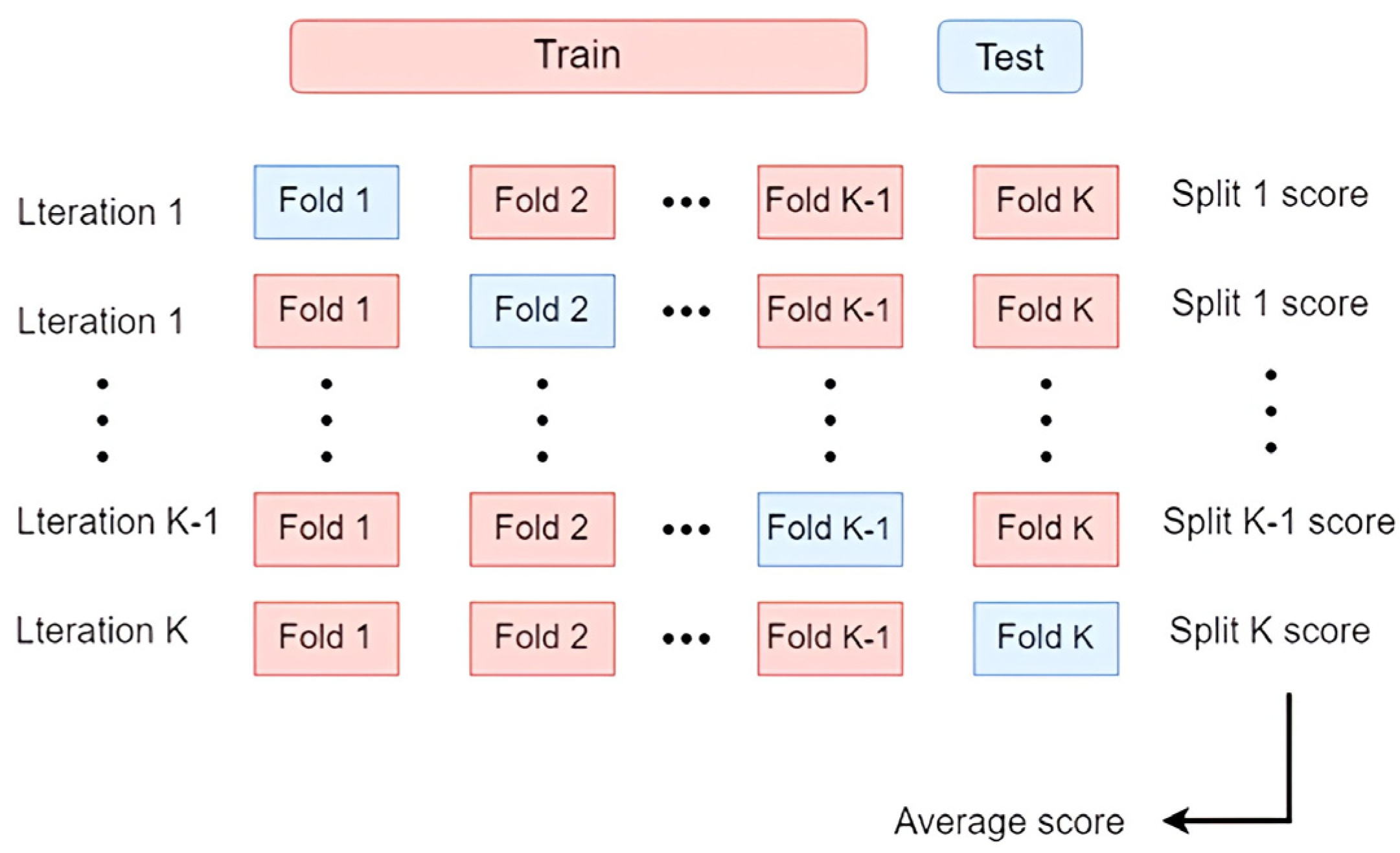
• Classifier training stage, where the feature dataset is evaluated using a support vector machine (SVM) combined with K-fold cross-validation

First, vibration signals along the X- and Y-axes were collected using accelerometers. To extract key fault features, WPD and EMD signal decomposition methods were employed to obtain decomposed features, which were then fused for both the X- and Y-axes. Subsequently, GSA was used to optimize the vibration features. After signal decomposition, the fused features from the X- and Y-axes were optimized using GSA, resulting in optimized features. These optimized features could then be used for model training and fault diagnosis.

During the signal decomposition and analysis process, let $D_v\in {\mathbb{R}}^{L_v\times N}$ represent the raw vibration signals, where $N$ denotes the number of samples and $L_v$ denotes the length of each sample in the vibration signal. The signals were then subjected to processing and analysis accordingly.

2.1. Signal Processing Stage

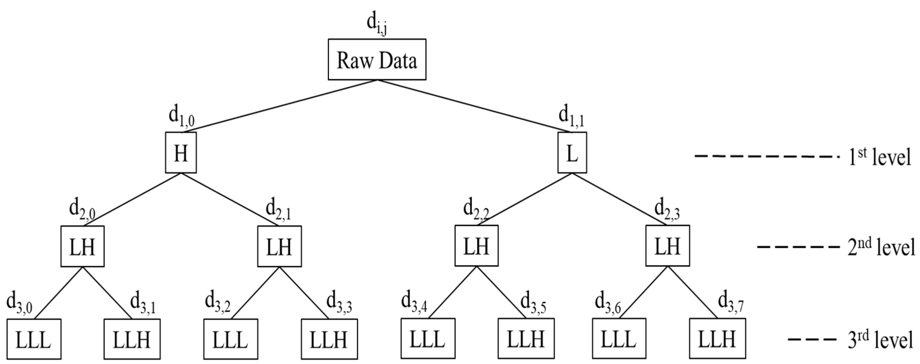
2.1.1. Feature Extraction Using WPD

The raw vibration signals are nonlinear in nature, making it difficult to rely solely on a single vibration signal for fault diagnosis. Therefore, feature extraction is a necessary and critical step in the fault diagnosis process. In this study, WPD is applied to the fault diagnosis of harmonic drives. By decomposing the signals into components of different frequencies, WPD reveals the time-frequency characteristics of the signals. The goal is to extract key fault features from both high-frequency and low-frequency signals.

When a raw signal is decomposed using WPD up to the third level, it is divided into 2, 4, and 8 nodes in the first, second, and third layers, respectively. The wavelet packet decomposition coefficients within each node contain diverse fault-related information across different frequency bands (both high and low frequencies), as shown in Figure 2. Additionally, different decomposition levels contain varying information related to faults. Relying solely on the wavelet decomposition at a single level to extract features makes it challenging to determine which level contains the most valuable information, and it is difficult to capture the fault characteristics of the signal fully. Therefore, to extract richer fault information, it is essential to derive vibration signal features from different levels of WPD. The steps for WPD feature extraction are described as follows: Step 1: Use WPD to decompose the vibration signal and obtain wavelet packet decomposition coefficients at different decomposition levels. Each level of WPD is denoted by $d_{i,j}\left[n\right]$, where $i$ represents a node at a specific level, $j$ represents the high (H) or low (L) frequency part within each node, and $\left[n\right]$ indicates the signal components contained in each node. Step 2: For each decomposition level, calculate the wavelet packet decomposition coefficients of the raw signal for each node. Therefore, with the maximum decomposition level $N$, the total number of features for a signal sample can be computed as ${(2}^0+2^1+2^2+2^3+\cdots +2^N)\times 1$.

2.1.2. Feature Extraction Using EMD

The decomposition process of EMD begins by detecting the local maxima and minima (negative peaks) within the signal. Then, interpolation is performed on the detected maxima and minima to obtain the upper and lower envelopes of the signal waveform. Afterward, the instantaneous mean line at each time point is calculated from the upper and lower envelopes. By subtracting the instantaneous mean from the signal waveform and repeating this process, the decomposition continues until the conditions for an intrinsic mode function (IMF) are satisfied. The steps for feature extraction using empirical mode decomposition (EMD) are described as follows: Step 1: Identify all the local maxima and minima of the raw vibration signal $D_v\left(t\right)$. Using cubic spline function interpolation, fit the upper envelope $e_{max}\left(t\right)$ based on the maxima and the lower envelope $e_{min}\left(t\right)$ based on the minima. The mean of the upper and lower envelopes, $m_1\left(t\right)$, is then calculated as shown in Equation (1):

$$m_1\left(t\right)={\displaystyle \frac{e_{max}\left(t\right)+e_{min}\left(t\right)}{2}}$$

(1)

Step 2: Identify the components of the IMF by ensuring that two conditions are met for the IMF definition. After satisfying these conditions, subtract the mean $m_1\left(t\right)$ from the original vibration signal sequence $D_v\left(t\right)$ to obtain a new signa $p_1^1\left(t\right)$, which removes the low-frequency component. This is represented by Equation (2):

$$p_1^1\left(t\right)=D_v\left(t\right)-m_1\left(t\right)$$

(2)

If Equation (2) does not meet the two conditions for the definition of an IMF after the first iteration, additional iterations are performed. After $k$ iterations, if the conditions of the IMF are satisfied, the first-order IMF component of the original vibration signal can be expressed as shown in Equation (3):

$$c_1\left(t\right)={IMF}_1\left(t\right)=p_1^k\left(t\right)$$

(3)

By subtracting the first IMF component $c_1\left(t\right)$ from the original vibration signal sequence, the new signal $r_1^1\left(t\right)$, which has removed the high-frequency component, can be obtained. This is represented by Equation (4):

$$r_1^1\left(t\right)=D_v\left(t\right)-c_1\left(t\right)$$

(4)

After iterating Equation (4), the process continues until $r_n\left(t\right)$ becomes a constant. The original vibration signal can then be decomposed using EMD and expressed as follows in Equation (5):

$$D_v\left(t\right)=\sum _{i=1}^n{c}_i\left(t\right)+r_n\left(t\right)$$

(5)

2.1.3. Comparison of Time Complexity for Signal Processing Methods

In the signal processing stage, two different signal decomposition methods were selected: WPD and EMD. Each method has its strengths and weaknesses in the feature extraction process, and the differences in their time complexities directly affect the computational efficiency of the overall system.

• WPD: The time complexity of WPD is $O\left(NlogN\right)$, where $N$ is the length of the signal. Since wavelet decomposition involves multi-level frequency decomposition, this method is computationally efficient for processing long-duration signals, making it suitable for multi-scale signal analysis.
• EMD: The time complexity of EMD is $(T_{EMD}·N)$, where $T_{EMD}$ represents the number of EMD iterations, and $N$ represents the signal length. Because EMD relies on repeated interpolation of the signal’s local maxima and minima, the computational load increases significantly as the complexity of the signal rises. This results in EMD having a higher time complexity compared to WPD, particularly when dealing with more intricate signals.

2.2. Feature Signal Enhancement Stage

After the original vibration signal $D_v\in {\mathbb{R}}^{L_v\times N}$ undergoes feature extraction using WPD and EMD, the resulting vibration decomposition features are denoted as $W_v\in {\mathbb{R}}^{D_v\times N}$.

2.2.1. Data Fusion

After feature extraction, the X-axis and Y-axis vibration decomposition features are represented as ${W_v\in {\mathbb{R}}^{D_v\times N}}_X$ and ${W_v\in {\mathbb{R}}^{D_v\times N}}_Y$, respectively. In this stage, a direct concatenation method is employed to perform multi-sensor data fusion. This process results in a new high-dimensional fused vibration feature ${{\mathcal{F}}_v\in {\mathbb{R}}^{D_v\times N}}_Z$, as shown in Equation (6):

$${{\mathcal{F}}_v\in {\mathbb{R}}^{D_v\times N}}_Z={W_v\in {\mathbb{R}}^{D_v\times N}}_X⨁{W_v\in {\mathbb{R}}^{D_v\times N}}_Y$$

(6)

When extending Equation (6) to accommodate $k$ sensors, the fused vibration feature becomes a concatenation of the decomposition features from all $k$ sensors. This can be expressed as shown in Equation (7):

$${{\mathcal{F}}_v\in {\mathbb{R}}^{D_v\times N}}_Z={W_v\in {\mathbb{R}}^{D_v\times N}}_{X\_1}⨁{W_v\in {\mathbb{R}}^{D_v\times N}}_{X\_2}\cdots ⨁{W_v\in {\mathbb{R}}^{D_v\times N}}_X\in {\mathbb{R}}^{(n1+n2+\cdots +nk)\times N}$$

(7)

2.2.2. Gravitational Search Algorithm

After obtaining the fused vibration features ${\mathcal{F}}_v\in {\mathbb{R}}^{D_v\times N}$, GSA is used to optimize the features. In the GSA optimization process, each solution is considered a mass-bearing object, and the entire set of solutions forms a system of objects that attract each other in the search space. The mass of each solution is determined by its fitness function value: the higher the fitness, the greater the mass. The solutions attract each other based on the laws of gravity, and this gravitational force guides the movement and dynamics of the solutions during the search process. In summary, GSA offers three major advantages in this study: (1) Global Search Capability: GSA is designed based on the laws of gravity, which allows for global exploration within the search space. This helps to avoid being trapped in local optima and increases the likelihood of finding the global optimum solution. (2) Adaptive Search Behavior: GSA dynamically adjusts parameters such as gravitational constant and acceleration, which enhances the optimization efficiency. For instance, applying GSA to the vibration decomposition features ${\mathcal{F}}_v\in {\mathbb{R}}^{D_v\times N}$, the mass function of the $i$-th vibration fusion feature in the $t$-th iteration, ${{\mathcal{f}}_{vM}}_i\left(t\right)$, is given by Equation (8). (3) Key Parameters in GSA: Two critical parameters in GSA, the initial gravitational value $G_0$ and the decay coefficient $\alpha$, play an essential role in the algorithm’s performance. As time progresses, the gravitational value decreases according to Equation (13), which indicates that the gravitational force is larger in the early stages, facilitating stronger global search capabilities. As the number of iterations increases, the gravitational value gradually decreases, helping the algorithm perform finer local searches in later stages. This design effectively prevents the algorithm from prematurely converging to a local optimum during the global search phase and maintains stability throughout the convergence process.

$${{\mathcal{f}}_{vM}}_i\left(t\right)={\displaystyle \frac{q_i\left(t\right)}{\sum _{j=1}^N{q}_j\left(t\right)}}$$

(8)

$$q_i\left(t\right)={\displaystyle \frac{{fit}_i\left(t\right)-worst\left(t\right)}{best\left(t\right)-worst\left(t\right)}}$$

(9)

The mass function for the i-th solution is given in Equation (9), where best and worst represent the highest and lowest fitness values, respectively, in the current iteration. This helps in determining the relative importance of each solution in the search process. The fitness function is calculated as shown in Equation (10):

$$fit\left(x\right)=\sum _{i\ne j}^n{\left(x_i-x_j\right)}^2$$

(10)

In this method, $x_i$ and $x_j$ represent two neighboring points in the same space. The squared distance between these two points is considered as the fitness function. The goal of using the squared distance is to amplify small differences, which helps in separating classes. Next, the gravitational force is calculated as shown in Equation (11):

$${\mathcal{f}}_v\_F_{ij}^d(t)=G(t){\displaystyle \frac{{\mathcal{f}}_v\_M_i\left(t\right){\mathcal{f}}_v\_M_j\left(t\right)}{R_{ij}(t)+\epsilon }}(x_j^d\left(t\right)-x_i^d(t))$$

(11)

where $G\left(t\right)$ is the gravitational constant that decreases over time; $R_{ij}\left(t\right)$ is the Euclidean distance between $i$ and $j$. $\epsilon$ is a small constant to avoid division by zero; and $i, j \in \left\{1, 2, 3, \dots , N\right\}$ and $i \ne j, \mathrm{w}\mathrm{i}\mathrm{t}\mathrm{h} d=1, 2, 3,\dots ,D$ represent the $d$-th dimension of the vibration feature. The force exerted on the $i$-th individual along the $d$-th dimension at iteration $t$ is given by Equation (12):

$${\mathcal{f}}_v\_F_i^d\left(t\right)=\sum _{j\in k_{best}, j\ne i}^N{rand}_j{F}_{ij}^d(t)$$

(12)

To reduce the time complexity caused by the high dimensionality during fusion, we adapt the gravitational constant $G\left(t\right)$ in Equation (10) to an adaptive gravitational calculation to save computational resources, as shown in Equation (13):

$$G\left(t\right)=G_0·exp\left(-\alpha ·{\displaystyle \frac{t}{T_{max}}}\right)$$

(13)

$G\left(t\right)$ is the gravitational constant at iteration $t$-th; $G_0$ is the initial gravitational constant (a positive constant); $\alpha$ is the gravitational decay factor;$t$ is the current iteration number; and $T_{max}$ and is the maximum number of iterations.

The velocity update Equation (14) and position update Equation (15) are given as follows:

$${D_{v}v}_i^d\left(t+1\right)=r\times {D_{v}v}_i^d\left(t\right)+D_v{a}_i^d\left(t\right)$$

(14)

$$D_v{x}_i^d\left(t+1\right)=D_v{x}_i^d\left(t\right)+{D_{v}v}_i^d\left(t+1\right)$$

(15)

GSA Optimization Process for Fused Features: Initialization: Randomly initialize the positions of individuals in the population and set the initial velocity to zero. Fitness Calculation: Use the fitness calculation formula Equation (9), where the Euclidean distance between adjacent variables is treated as the fitness function. Mass and Gravity Calculation: Update the mass of each individual based on fitness values and compute the gravitational force using Equations (11) and (13). This directs the search towards a better set of features. Acceleration and Velocity Calculation: Update the acceleration and velocity using the gravitational force and the respective formulas. Position Update: With the updated velocity, calculate the new position for the next iteration using Equation (15). This process ensures that the optimization through GSA refines the fused features to maximize the effectiveness of fault diagnosis by iteratively searching for the optimal solution.

2.2.3. Time Complexity of the Optimization Algorithm

In the feature optimization process, we employed the GSA to handle the selection and optimization of high-dimensional data features.

The $\mathrm{i}\mathrm{t}\mathrm{e}\mathrm{r}\mathrm{a}\mathrm{t}\mathrm{i}\mathrm{o}\mathrm{n}\mathrm{s}$ refers to the maximum number of iterations the algorithm can perform, $\mathrm{p}\mathrm{o}\mathrm{p}\mathrm{u}\mathrm{l}\mathrm{a}\mathrm{t}\mathrm{i}\mathrm{o}\mathrm{n}$ size indicates the number of solutions in the solution set, and $\mathrm{d}\mathrm{i}\mathrm{m}\mathrm{e}\mathrm{n}\mathrm{s}\mathrm{i}\mathrm{o}\mathrm{n}$ represents the dimensionality of the feature space. Compared to particle swarm optimization (PSO) and the genetic algorithm (GA), GSA can maintain strong global search capabilities even with fewer iterations. More specifically, under the same feature space dimensionality, GSA demonstrates a robust ability to explore the global solution space. Even with a smaller number of iterations and a reduced population size, GSA can still reach the global optimum. Therefore, compared to other optimization algorithms, such as PSO and GA, GSA offers a more stable and faster convergence while maintaining global search capabilities.

PSO has a time complexity similar to that of GSA, but it is more prone to becoming trapped in local optima, especially in high-dimensional spaces. PSO often requires more iterations to escape local optima and find a global solution.

GA updates solutions in each iteration through selection, crossover, and mutation operations. While GA can maintain population diversity, its convergence speed is slower, particularly when the chromosome length increases, which leads to a significant rise in computational complexity.

In contrast, GSA can achieve the global optimum with fewer iterations, making it particularly suitable for dealing with high-dimensional data and nonlinear problems. This advantage makes GSA highly efficient for complex data optimization tasks. In summary, GSA provides a unique balance between efficient global exploration and quick convergence, which sets it apart from PSO and GA. Its ability to reach the global optimum with fewer iterations and smaller population sizes makes it ideal for high-dimensional and nonlinear data scenarios.

To further reduce the computational resource waste during high-dimensional data processing, we introduced adaptive gravitational calculation (Equation (13)), which dynamically adjusts the gravitational force throughout the iterative process. This approach minimizes unnecessary computational overhead. The adaptive gravitational force is adjusted based on the current iteration; as the number of iterations increases, the gravitational value gradually decreases. This allows for broader global exploration in the early stages of the optimization, followed by finer local search as the algorithm converges.

2.3. SVM and K-Fold Cross-Validation

This study categorizes the failure modes of harmonic drives (

Table 1. Fault types and causes for harmonic drives.

Fault Model	Gear Wear	Less Grease	Gear Fracture	Improper Load	Bearing Damage
Fault Cause	Excessive shaft misalignment, high surface roughness	Excessive or less grease	Overloading, misuse	Excessive load	Bearing ball wear

) and then uses the GSA-optimized vibration features to train a SVM for classification tasks. The strength of SVM lies in its robust ability to separate data in high-dimensional spaces, making it particularly suitable for datasets that are not linearly separable. SVM can effectively handle high-dimensional data and performs well in small sample sizes. It offers strong generalization capabilities and accuracy for classification tasks with low noise and clear boundaries, making it ideal for identifying various health conditions of harmonic drives.

During the training of the SVM fault classifier, the process begins by extracting multi-level features from the signals of various fault types. These features are then fused, followed by optimization using GSA. The optimized features are subsequently input into the SVM to obtain the final classification results.

To achieve a fair evaluation of the model, K-fold cross-validation was adopted for model training in this research. In the K-fold cross-validation process, the original dataset is randomly divided into $K$ equally proportioned subsets. In each training iteration, $K-1$ subsets are selected as the training set, and the remaining subset is used as the test set for validation. This process is repeated $K$ times, ensuring that each subset serves as the test set in different iterations. Finally, the test results from all iterations are combined for a comprehensive analysis, providing a more robust and reliable evaluation of the model’s performance. This approach effectively reduces the risk of overfitting and enhances the model’s generalization ability.

3. Experimental Study

A custom test setup was designed to simulate the harmonic drive of the sixth axis of a robotic arm, and data collection was performed using this test apparatus (Figure 3a,b). This setup allowed us to gather relevant vibration and operational data under various fault conditions, providing a controlled environment for evaluating the performance of the proposed fault diagnosis method.

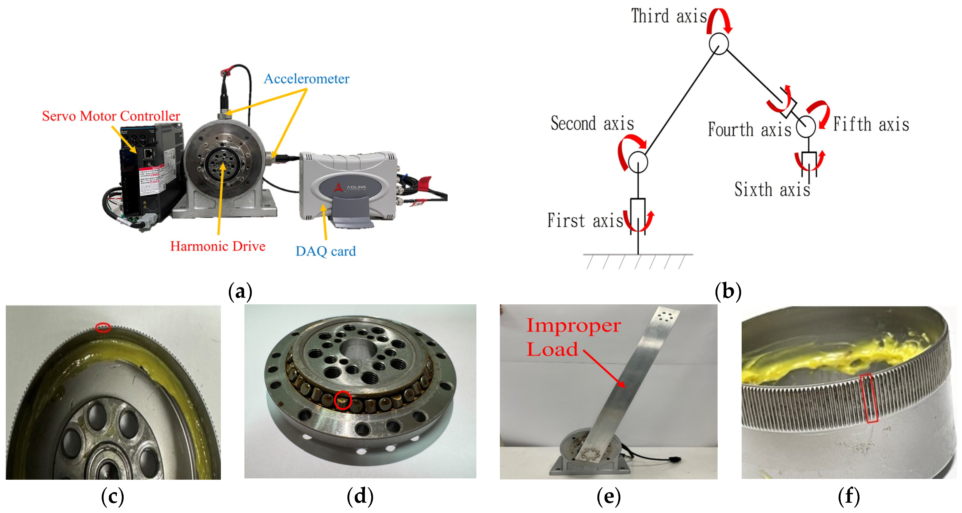
3.1. Experimental Setup

Figure 3a illustrates the custom-designed test apparatus for the sixth-axis harmonic drive, which aims to simulate the operation of the sixth axis in a real robotic arm. The setup consists of three main units:

• Harmonic Drive Unit: This unit uses a harmonic drive to mimic the motion of the robotic arm’s sixth axis. It comprises an ECM-B3M-C20604 servo motor and a harmonic drive with a reduction ratio of 100.
• Control Unit: The servo motor is controlled by an ASD-B3-0421-L servo drive controller to manage the motor’s operation.
• Data Acquisition Unit: The ADLink USB-2405 device is employed to collect vibration data from the X- and Y-axes.

To accurately detect the health status of the harmonic drive, we manually simulated six common operating conditions, including one normal condition (N) and five single-point fault conditions: gear wear (GW) (Figure 3c), bearing damage (B) (Figure 3d), improper load (IL) (Figure 3e), gear fracture (GF) (Figure 3f), and less grease (LG). For precise verification of the harmonic drive’s health, vibration data were collected at a sampling rate of 51.2 kHz for all six operating conditions. Additionally, 170 samples were gathered at a rotational speed of 2400 rpm, with each sample having a duration of 1 s (

Table 2. Number of original data entries for vibration signals.

Model Type	Signal Type	Total
N, GF, GW, IL, LG, B	Vibration	170

). The time-domain profiles of signals from different health conditions are similar, making it quite challenging to distinguish between these states based solely on raw measured signals. Therefore, signal processing algorithms are required to extract effective fault features. During the model training phase, 5-fold cross-validation was adopted. The dataset was randomly and uniformly divided into five subsets. One subset was randomly selected as the test set, and the remaining four were used as the training set. This process was repeated five times, with each subset serving as the test set once. The average result of these five tests was used as the final evaluation of the model’s performance (Figure 4).

3.2. Experimental Procedure

• Step 1: Collect vibration signals from the harmonic drive under six fault models: normal gear, gear wear, gear fracture, less grease, bearing damage, and improper load. The signals are then decomposed using WPD and EMD to obtain decomposition features.
• Step 2: Fuse the decomposition feature matrices from both the X-axis and Y-axis.
• Step 3(a): Perform SVM classification on the fused features, applying 5-fold cross-validation to ensure fairness in training.
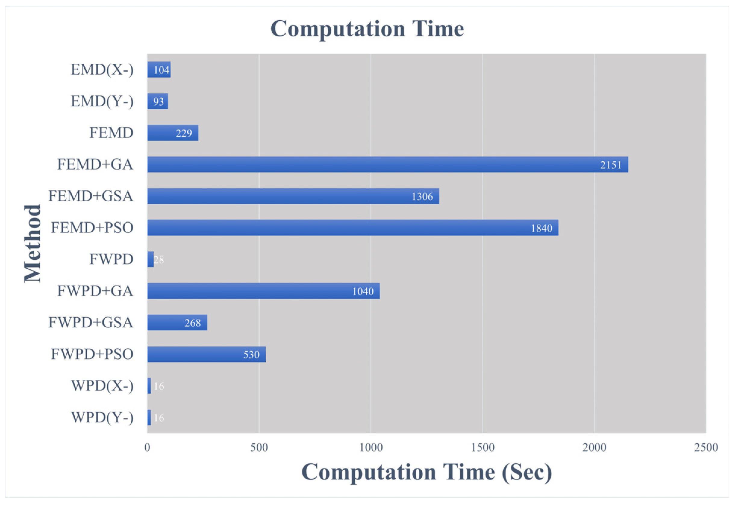
• Step 3(b): Optimize the fused features using GSA, PSO, and GA, and compute the computation time performance of each method.
• Step 4: Use the optimized features from step 3(b) for SVM classification, again employing 5-fold cross-validation to ensure fair training.

4. Data Analysis Experiment

The raw vibration signals are nonlinear, making it challenging to rely on a single signal for fault diagnosis. Therefore, feature extraction is a necessary and crucial step in the fault diagnosis process. Two signal decomposition methods were employed to extract key features: WPD; the propose method further decomposes the signal into high-frequency and low-frequency components. Its significant advantage lies in its multi-scale analysis capability, which can capture features across different frequency ranges, making it especially suitable for time-frequency analysis. EMD begins by detecting the local maxima and minima of the signal and interpolating these points to form the upper and lower envelopes of the signal waveform. From these envelopes, the instantaneous mean line at each time point is calculated. This process is repeated until the conditions for the IMF are met.

4.1. Computational Complexity Analysis

A combination of WPD and EMD methods was employed alongside optimization algorithms such as GSA, PSO, and GA to validate the proposed WPD-GSA diagnostic framework. However, a common drawback of data fusion is the potential for imbalanced data and high-dimensional issues, which can lead to increased computational complexity and a significant waste of computational resources.

4.2. Performance Evaluation

The proposed method first extracts features from vibration signals for different axes and operating conditions using WPD and EMD. Then, the extracted features from the X-axis and Y-axis are fused, followed by feature optimization using GSA. For a comprehensive comparison, we evaluated WPD, EMD, and their fused versions, FWPD and FEMD. Finally, GSA was applied to optimize the fused features FWPD and FEMD. In this section, we compare the diagnostic performance of WPD, EMD, FWPD, and FEMD and the results after applying different optimization algorithms to the signal features. According to the experimental results,

Table 3. Performance evaluation of different diagnostic methods.

Methods	Vibration
	ACC	PC	RC	F1	Computation Time
EMD (X-axis)	52.6	52.2	56.6	50.6	104.11(S)
EMD (Y-axis)	35.6	40.5	35.6	33.7	92.66(S)
WPD (X-axis)	68.6	69.7	68.6	88.6	15.6(S)
WPD (Y-axis)	55.0	55.2	55.0	54.4	15.87(S)
FEMD	65.0	75.8	65.0	64.84	228.67(S)
FEMD+GSA	88.5	89.7	88.5	86.9	1306.02(S)
FEMD+GA	78.6	79.3	78.3	77.5	2151.39(S)
FEMD+PSO	82.3	83.7	82.5	82.5	1839.63(S)
FWPD	73.3	75.1	73.3	71.7	28.35(S)
FWPD+GSA	93.3	94.5	93.3	92.9	267.95(S)
FWPD+GA	80.76	82.2	80.7	80.4	1040.46(S)
FWPD+PSO	76.6	78.1	76.6	77.0	530.33(S)

shows the diagnostic performance of various methods. The performance of WPD and EMD is inferior to that of the fused FWPD and FEMD. However, as the feature dimensionality increases, the time complexity also rises significantly.

The experimental results in Figure 5 indicate that whether using WPD or EMD alone or after feature fusion with FWPD and FEMD, the accuracy and diagnostic performance differ. Both WPD and EMD exhibited classification errors in certain fault types, particularly in distinguishing between gear fracture and gear wear, where the similarities in features led to higher misclassification rates. However, after feature fusion (FWPD and FEMD) and optimization, these errors were significantly reduced. To address this issue, we introduced different optimization algorithms. The results in Figure 6 show that GSA significantly outperforms GA and PSO in terms of diagnostic accuracy. Specifically, FWPD combined with GSA achieved an accuracy of 93.3%, while FWPD+GA and FWPD+PSO achieved 80.76% and 76.6%, respectively. Although GA improved accuracy, its computation time was much higher than that of GSA, highlighting GSA’s potential for computation-time applications. Figure 7 demonstrates the performance of different methods in terms of computation time processing. GSA not only improved diagnostic accuracy but also maintained lower computational resource consumption, making it more practical for industrial applications. Notably, in the FWPD+GSA combination, the classification accuracy for gear fracture and gear wear improved substantially, indicating that GSA optimization of fused features effectively mitigates feature similarity issues and enhances diagnostic accuracy. As shown in Figure 6, the diagnostic performance after feature fusion is improved compared to using WPD or EMD individually. However, with feature fusion, the dimensionality increases, leading to a noticeable rise in time complexity. To further enhance diagnostic accuracy and reduce the waste of computational resources, we employed optimization algorithms for feature selection. With the inclusion of GSA, accuracy and other performance metrics improved significantly, with the FWPD+GSA combination outperforming all other methods in all tests.

However, although the optimization methods GSA, PSO, and GA improved diagnostic performance, their computation times increased significantly. In comparison, the diagnostic method using GSA achieved high accuracy while maintaining relatively low computational overhead. Based on the experimental results, the proposed WPD-GSA diagnostic framework effectively enhances fault diagnosis accuracy. Moreover, compared to other optimization methods, GSA demonstrates lower computational load, highlighting its potential for practical applications.

5. Conclusions

This research presents a multi-sensor data fusion method enhanced by WPD and the GSA for fault diagnosis in harmonic drives. As industrial equipment such as robotic arms grows increasingly complex, the need for more accurate fault diagnosis in critical components like harmonic drives has become more pressing. Single-sensor data often lacks sufficient information for accurate fault detection, so this research improves diagnostic accuracy by employing multi-sensor data fusion. Specifically, WPD was used to decompose X-axis and Y-axis vibration signals, extracting multi-scale high- and low-frequency features. After fusing the features from both axes, GSA was applied to optimize the high-dimensional fused features. Experimental results showed that feature fusion significantly enhanced diagnostic accuracy compared to using WPD or empirical mode decomposition (EMD) alone. Through multiple experiments, the study demonstrated the effectiveness of feature fusion methods, with FWPD and FEMD improving both diagnostic accuracy and stability. The FWPD+GSA combination achieved the highest diagnostic accuracy at 93.3%, surpassing WPD+GA (80.76%) and FWPD+PSO (76.6%). GSA’s global search capability and efficiency enabled it to maintain high accuracy with a lower computational burden, offering good convergence speed and computation time performance. However, while feature fusion improves diagnostic accuracy, it also increases computational load. GSA effectively mitigates this by reducing redundant features and minimizing overfitting risks through adaptive gravity. In contrast, GA and PSO, although improving accuracy, require significantly more computation time, particularly GA, which struggles with high-dimensional data.

References

1. IFR International Federation of Robotics. World Robotics 2023 Report: Asia Ahead of Europe and the Americas. Available online: https://ifr.org/ifr-press-releases/news/world-robotics-2023-report-asia-ahead-of-europe-and-the-americas (accessed on 29 November 2023).
2. Raviola, A.; De Martin, A.; Guida, R.; Jacazio, G.; Mauro, S.; Sorli, M. Harmonic drive gear failures in industrial robots applications: An overview. In Proceedings of the PHM Society European Conference, Virtual, 28 June–2 July 2021; p. 11. [Google Scholar]
3. Li, Q. RUL estimation for rolling bearings using augmented quaternion-based least mean P-power with correntropy induced metric under framework of sparsity. IEEE/ASME Trans. Mechatron. 2022, 28, 976–989. [Google Scholar] [CrossRef]
4. Zio, E. Prognostics and Health Management (PHM): Where are we and where do we (need to) go in theory and practice. Reliab. Eng. Syst. Saf. 2022, 218, 108119. [Google Scholar] [CrossRef]
5. Medoued, A.; Mordjaoui, M.; Soufi, Y.; Sayad, D. Induction machine bearing fault diagnosis based on the axial vibration analytic signal. Int. J. Hydrogen Energy 2016, 41, 12688–12695. [Google Scholar] [CrossRef]
6. Cui, L.; Yan, L.; Zhao, D. Instantaneous Frequency Estimation-Based Order Tracking for Bearing Fault Diagnosis Under Strong Noise. IEEE Sens. J. 2023, 23, 30940–30949. [Google Scholar] [CrossRef]
7. Paskalovski, S.; Digalovski, M. Simulation models for induction machine protection analysis. Int. J. Inf. Technol. Secur. 2022, 14, 63–74. [Google Scholar]
8. Hou, X.; Du, F.; Huang, K.; Qiu, J.; Zhong, X. A Current-Based Fault Diagnosis Method for Rotating Machinery with Limited Training Samples. IEEE Trans. Instrum. Meas. 2023, 72, 3530414. [Google Scholar] [CrossRef]
9. Raouf, I.; Lee, H.; Kim, H.S. Mechanical fault detection based on machine learning for robotic RV reducer using electrical current signature analysis: A data-driven approach. J. Comput. Des. Eng. 2022, 9, 417–433. [Google Scholar] [CrossRef]
10. Wang, T.; Liang, M.; Li, J.; Cheng, W.; Li, C. Bearing fault diagnosis under unknown variable speed via gear noise cancellation and rotational order sideband identification. Mech. Syst. Signal Process. 2015, 62, 30–53. [Google Scholar] [CrossRef]
11. Visnadi, L.B.; de Castro, H.F. Influence of bearing clearance and oil temperature uncertainties on the stability threshold of cylindrical journal bearings. Mech. Mach. Theory 2019, 134, 57–73. [Google Scholar] [CrossRef]
12. Choudhary, A.; Goyal, D.; Letha, S.S. Infrared Thermography-Based Fault Diagnosis of Induction Motor Bearings Using Machine Learning. IEEE Sens. J. 2021, 21, 1727–1734. [Google Scholar] [CrossRef]
13. Cui, X.; Wu, Y.; Zhang, X.; Huang, J.; Wong, P.K.; Li, C. A novel fault diagnosis method for rotor-bearing system based on instantaneous orbit fusion feature image and deep convolutional neural network. IEEE/ASME Trans. Mechatron. 2022, 28, 1013–1024. [Google Scholar] [CrossRef]
14. Xia, M.; Li, T.; Xu, L.; Liu, L.; De Silva, C.W. Fault diagnosis for rotating machinery using multiple sensors and convolutional neural networks. IEEE/ASME Trans. Mechatron. 2017, 23, 101–110. [Google Scholar] [CrossRef]
15. Kumar, P.; Raouf, I.; Kim, H.S. Transfer learning for servomotor bearing fault detection in the industrial robot. Adv. Eng. Softw. 2024, 194, 103672. [Google Scholar] [CrossRef]
16. Kibrete, F.; Engida Woldemichael, D.; Shimels Gebremedhen, H. Multi-Sensor data fusion in intelligent fault diagnosis of rotating machines: A comprehensive review. Measurement 2024, 232, 114658. [Google Scholar] [CrossRef]
17. AlShorman, O.; Irfan, M.; Abdelrahman, R.e.B.; Masadeh, M.; Alshorman, A.; Sheikh, M.A.; Saad, N.; Rahman, S. Advancements in condition monitoring and fault diagnosis of rotating machinery: A comprehensive review of image-based intelligent techniques for induction motors. Eng. Appl. Artif. Intell. 2024, 130, 107724. [Google Scholar] [CrossRef]
18. Fang, R.; Liu, Z.; Peng, C.; Yang, Y.; Zhang, S. Fault diagnosis of inter-turn short circuit in turbogenerator rotor windings based on vibration-current signal fusion. Energy Rep. 2023, 9, 316–323. [Google Scholar] [CrossRef]
19. Gan, C.; Wu, J.; Yang, S.; Hu, Y.; Cao, W.; Si, J. Fault diagnosis scheme for open-circuit faults in switched reluctance motor drives using fast Fourier transform algorithm with bus current detection. IET Power Electron. 2016, 9, 20–30. [Google Scholar] [CrossRef]
20. Gao, Z.; Cecati, C.; Ding, S.X. A survey of fault diagnosis and fault-tolerant techniques—Part I: Fault diagnosis with model-based and signal-based approaches. IEEE Trans. Ind. Electron. 2015, 62, 3757–3767. [Google Scholar] [CrossRef]
21. Habbouche, H.; Benkedjouh, T.; Zerhouni, N. Intelligent prognostics of bearings based on bidirectional long short-term memory and wavelet packet decomposition. Int. J. Adv. Manuf. Technol. 2021, 114, 145–157. [Google Scholar] [CrossRef]
22. Babu, T.N.; Devendiran, S.; Aravind, A.; Rakesh, A.; Jahzan, M. Fault diagnosis on journal bearing using empirical mode decomposition. Mater. Today Proc. 2018, 5, 12993–13002. [Google Scholar] [CrossRef]
23. Wang, D.; Zhao, Y.; Yi, C.; Tsui, K.-L.; Lin, J. Sparsity guided empirical wavelet transform for fault diagnosis of rolling element bearings. Mech. Syst. Signal Process. 2018, 101, 292–308. [Google Scholar] [CrossRef]
24. Yan, R.; Shang, Z.; Xu, H.; Wen, J.; Zhao, Z.; Chen, X.; Gao, R.X. Wavelet transform for rotary machine fault diagnosis: 10 years revisited. Mech. Syst. Signal Process. 2023, 200, 110545. [Google Scholar] [CrossRef]
25. de Azevedo, H.D.M.; Araújo, A.M.; Bouchonneau, N. A review of wind turbine bearing condition monitoring: State of the art and challenges. Renew. Sustain. Energy Rev. 2016, 56, 368–379. [Google Scholar] [CrossRef]
26. Chudzik, A.; Warda, B. Effect of radial internal clearance on the fatigue life of the radial cylindrical roller bearing. Eksploat. I Niezawodn. 2019, 21, 211–219. [Google Scholar] [CrossRef]
27. Karabacak, Y.E.; Gürsel Özmen, N.; Gümüşel, L. Intelligent worm gearbox fault diagnosis under various working conditions using vibration, sound and thermal features. Appl. Acoust. 2022, 186, 108463. [Google Scholar] [CrossRef]
28. Han, T.; Liu, C.; Yang, W.; Jiang, D. A novel adversarial learning framework in deep convolutional neural network for intelligent diagnosis of mechanical faults. Knowl. -Based Syst. 2019, 165, 474–487. [Google Scholar] [CrossRef]
29. Irfan, M.; Althobiani, F.; Alwadie, A.S.; Zaffar, M.; Abbass, A.; Glowacz, A.; Ghonaim, S.M.; Abdushkour, H.; Rahman, S.; Alshorman, O. Condition monitoring of water pump bearings using ensemble classifier. Adv. Mech. Eng. 2022, 14, 16878132221089170. [Google Scholar] [CrossRef]
30. Dameshghi, A.; Refan, M.H. Wind turbine gearbox condition monitoring and fault diagnosis based on multi-sensor information fusion of SCADA and DSER-PSO-WRVM method. Int. J. Model. Simul. 2019, 39, 48–72. [Google Scholar] [CrossRef]
31. Lei, Y.; Lin, J.; He, Z.; Zuo, M.J. A review on empirical mode decomposition in fault diagnosis of rotating machinery. Mech. Syst. Signal Process. 2013, 35, 108–126. [Google Scholar] [CrossRef]
32. Sun, H.; Zi, Y.; He, Z. Wind turbine fault detection using multiwavelet denoising with the data-driven block threshold. Appl. Acoust. 2014, 77, 122–129. [Google Scholar] [CrossRef]
33. Rashedi, E.; Nezamabadi-Pour, H.; Saryazdi, S. GSA: A gravitational search algorithm. Inf. Sci. 2009, 179, 2232–2248. [Google Scholar] [CrossRef]
34. Rashedi, E.; Rashedi, E.; Nezamabadi-pour, H. A comprehensive survey on gravitational search algorithm. Swarm Evol. Comput. 2018, 41, 141–158. [Google Scholar] [CrossRef]
35. Ding, S.; Hao, M.; Cui, Z.; Wang, Y.; Hang, J.; Li, X. Application of multi-SVM classifier and hybrid GSAPSO algorithm for fault diagnosis of electrical machine drive system. ISA Trans. 2023, 133, 529–538. [Google Scholar] [CrossRef] [PubMed]
36. Precup, R.-E.; David, R.-C.; Petriu, E.M.; Radac, M.-B.; Preitl, S. Adaptive GSA-based optimal tuning of PI controlled servo systems with reduced process parametric sensitivity, robust stability and controller robustness. IEEE Trans. Cybern. 2014, 44, 1997–2009. [Google Scholar] [CrossRef] [PubMed]
37. Eappen, G.; Shankar, T. Hybrid PSO-GSA for energy efficient spectrum sensing in cognitive radio network. Phys. Commun. 2020, 40, 101091. [Google Scholar] [CrossRef]
38. Hooda, H.; Verma, O.P. Fuzzy clustering using gravitational search algorithm for brain image segmentation. Multimed. Tools Appl. 2022, 81, 29633–29652. [Google Scholar] [CrossRef]
39. Zamfirache, I.A.; Precup, R.-E.; Roman, R.-C.; Petriu, E.M. Reinforcement Learning-based control using Q-learning and gravitational search algorithm with experimental validation on a nonlinear servo system. Inf. Sci. 2022, 583, 99–120. [Google Scholar] [CrossRef]
40. Raouf, I.; Lee, H.; Noh, Y.R.; Youn, B.D.; Kim, H.S. Prognostic health management of the robotic strain wave gear reducer based on variable speed of operation: A data-driven via deep learning approach. J. Comput. Des. Eng. 2022, 9, 1775–1788. [Google Scholar] [CrossRef]
41. Das, O.; Bagci Das, D.; Birant, D. Machine learning for fault analysis in rotating machinery: A comprehensive review. Heliyon 2023, 9, e17584. [Google Scholar] [CrossRef]
42. Raouf, I.; Kumar, P.; Soo Kim, H. Deep learning-based fault diagnosis of servo motor bearing using the attention-guided feature aggregation network. Expert Syst. Appl. 2024, 258, 125137. [Google Scholar] [CrossRef]
43. Siddique, M.F.; Ahmad, Z.; Ullah, N.; Kim, J. A Hybrid Deep Learning Approach: Integrating Short-Time Fourier Transform and Continuous Wavelet Transform for Improved Pipeline Leak Detection. Sensors 2023, 23, 8079. [Google Scholar] [CrossRef] [PubMed]
44. Zhu, Z.; Lei, Y.; Qi, G.; Chai, Y.; Mazur, N.; An, Y.; Huang, X. A review of the application of deep learning in intelligent fault diagnosis of rotating machinery. Measurement 2023, 206, 112346. [Google Scholar] [CrossRef]
45. Siddique, M.F.; Ahmad, Z.; Kim, J.-M. Pipeline leak diagnosis based on leak-augmented scalograms and deep learning. Eng. Appl. Comput. Fluid Mech. 2023, 17, 2225577. [Google Scholar] [CrossRef]
46. Raouf, I.; Kumar, P.; Lee, H.; Kim, H.S. Transfer Learning-Based Intelligent Fault Detection Approach for the Industrial Robotic System. Mathematics 2023, 11, 945. [Google Scholar] [CrossRef]
Figure 1. Enhanced harmonic drive fault diagnosis framework diagram.
Machines 12 00831 g001
Figure 2. Three-layered wavelet packet decomposition process diagram.
Machines 12 00831 g002
Figure 3. (a) Experimental setup; (b) schematic of the sixth axis; (c) gear wear; (d) bearing damage; (e) improper load; (f) gear fracture.
Machines 12 00831 g003
Figure 4. K-fold cross-validation diagram.
Machines 12 00831 g004
Figure 5. Accuracy comparison chart for different optimization methods. (a) FWPD, (b) FWPD+GSA, (c) FEMD, (d) FEMD+GSA.
Machines 12 00831 g005
Figure 6. Accuracy comparison chart.
Machines 12 00831 g006
Figure 7. Computation time comparison of different methods.
Machines 12 00831 g007