Research on Optimal Design of Ultra-High-Speed Motors Based on Multi-Physical Field Coupling Under Mechanical Boundary Constraints

Abstract

This study investigates the impact of rotor structure, material selection, and cooling methods on ultra-high-speed motor performance, revealing performance variation laws under multi-physical field coupling. Considering mechanical boundary constraints, we propose an optimization design method based on a multi-physical field coupling model. Using a MaxPro experimental design, initial samples are obtained and fitted using a Kriging surrogate model. The NSGA-2 algorithm is then applied for optimization, with Relative Maximum Absolute Error (RMAE) and Relative Average Absolute Error (RAAE) employed for accuracy evaluation. The Kriging model is iteratively updated based on evaluation results until the optimal design is achieved. This method enhances motor performance, ensures mechanical boundary conditions, and reduces computational load. Experimental results show significant improvements in efficiency and power density. This study provides theoretical support and technical guidance for ultra-high-speed motor design and offers new ideas for related motor research and development. Future work will explore more efficient and intelligent optimization algorithms to continuously advance ultra-high-speed motor technology.

1. Introduction

The rotor speed of high-speed motors is usually higher than 10,000 r/min, which has the advantages of high power density, small size, fast dynamic response, direct connection with high-speed loads, and high transmission efficiency [1]. It will be widely used in aviation [2,3,4,5,6], automotive [7,8,9,10,11,12], and other fields.

However, the operating characteristics of this high-speed motor are significantly different from ordinary motors [13]. Hence, during the process of optimizing design, it is imperative to take into account various factors, such as rotor strength, dynamic attributes, and core loss.

(1)

Rotor strength. In the rotor of ultra-high-speed motors, permanent magnets are their weak point, and the issue of how to design permanent magnet protective covers is a research hotspot [14,15,16]. The most commonly used protective measures are to use carbon fiber to bind the permanent magnets [17,18] and to add a high-strength non-magnetic alloy protective cover outside the permanent magnets [19,20]. These two materials have different effects on the performance of the motor sleeve, which needs to be carefully considered in the design [21,22,23], such as the impact on heat dissipation [20,21,23] and the eddy current effect [15,20,24,25].

(2)

Dynamic attributes. When designing a high-speed motor, it is necessary to consider the dynamic characteristics of the rotor system [26], such as the effects of rotor magnetization methods and rotor support structures on cogging torque and rotor dynamics [27], and how to improve the critical speed of the rotor [7]

(3)

Core Loss. The increase in stator iron loss and rotor eddy current loss caused by high speed [15,16,28] requires detailed research. Optimizing the stator structure [15], adopting centralized winding [29], using new motor integrated permanent magnet gear [30], optimizing the permanent magnet sleeve [31], and using a split-phase winding method [32] can all reduce the losses of high-speed motors.

From the above analysis, it can be seen that multiple physical fields such as electromagnetics, mechanics, and thermotics must be considered in the design process of ultra-high-speed motors, making the design process more complex. Recently, the multi-physics coupling optimization design of motors has become a research hotspot.

Firstly, understanding the coupling mechanism of multiple physical fields and establishing a coupling model for these fields are crucial for the design of ultra-high-speed motors [33,34,35,36,37,38,39]. Generally, when optimizing the design of high-speed motors, samples are obtained using a Latin hypercube experimental design [40], and the Kriging method [12,40,41,42,43] is employed to fit an approximate model. Then, genetic optimization algorithms [40,44], Taguchi Method [45], NLPQL algorithm [35], particle swarm optimization [46], or adaptive particle swarm optimization [47] are used for motor optimization design.

It can be seen that the issue of how to improve the accuracy and calculation speed of the multi-physical field coupling model for ultra-high-speed motors, and achieve a global optimization design, is a problem that needs to be solved in current research and has become a hot research topic.

2. Motor Topology

Ultra-high-speed motors increase the frequency of magnetic field alternating and cause an increase in iron loss. Generally, one or two pairs of permanent magnets are used, and for internal rotor motors, carbon fiber sleeves need to be designed. The topology structure of the motor studied in this article is shown in Figure 1, which adopts a one-pair pole, inner rotor, 18 slots, and distributed winding structure.

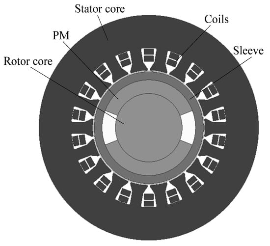
Figure 1. Motor topology.

The specific design indicators are shown in Table 1, and the initial design parameters are shown in Table 2.

Table 1. Design indicators.

Parameters	Value
Rated line voltage (V)	380
Rated power (kW)	12
Rated speed (r/min)	100,000
Rated efficiency (%)	>95

Table 2. Design parameters.

Parameters	Value (mm)
Outer diameter of stator (Do1)	110
Outer diameter of rotor core (D)	40
Armature length (Lef)	48
Thickness of permanent magnet (hNd)	2
Sleeve thickness (hsleeve)	2
Air gap length (LAirgap)	0.8

3. Mechanical Modeling and Analysis of Motor Rotors

3.1. Rotor Dynamics Model

The simplified rotor-bearing system mainly includes shaft segments, rigid discs, and bearings, as shown in Figure 2.

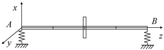
Figure 2. Typical dynamic model of rotor bearing system.

The rotor motion equation can be expressed as follows:

$$\mathit{M}\ddot{\mathit{u}}+\mathit{G}\dot{\mathit{u}}+\mathit{K}\mathit{u}=\mathit{Q}$$

(1)

where M is mass matrix, G is gyroscopic matrix, K is stiffness matrix, u is generalized coordinate, and Q is generalized force. M and K are real symmetric positive definite matrices, and G is a real anti symmetric matrix. The critical angular velocity of the synchronous forward vortex can be obtained by solving the frequency equation.

3.2. Calculation of Critical Speed and Vibration Mode of a Single Rotor

Table 3 provides the preliminary rotor parameters. The permanent magnet part has three layers, which are the steel shaft, the permanent magnet, and the sleeve. The other parts only have one layer, which is the steel shaft. Therefore, the thickness and density of the second and third layers of these parts are 0. Then, the rotor length is 288.5 mm, the mass is 1.685 kg, the thickness of the permanent magnet is 1 mm, and the thickness of the sleeve is 1 mm. Set the bearing stiffness to $1\times {10}^6\mathrm{N}/\mathrm{m}$, the imbalance level to G2.5 (100,000 rpm), and the rotor imbalance to 0.4 gmm. The imbalance force is evenly distributed on the two impellers, with an angle of 90° for the imbalance amount.

Table 3. Rotor parameters.

First Layer (Steel)		Second Layer (PM)		Third Layer (Carbon Fiber)		L/mm	Number of Segments	Notes
D1/mm	$\mathit{\rho }$1/kg/m3	D2/mm	$\mathit{\rho }$2/kg/m3	D3/mm	$\mathit{\rho }$3/kg/m3
12	7850	12	0	12	0	18	1
40	7850	40	0	40	0	26	2	Impeller position
20	7850	20	0	20	0	21	1
24	7850	24	0	24	0	30	2	Bearing position
24	7850	24	0	24	0	20	1
38	7850	38	0	38	0	9.1	1
38	7850	40	8400	42	1600	56.3	3	Magnetic pole position
38	7850	38	0	38	0	9.1	1
24	7850	24	0	24	0	9	1
24	7850	24	0	24	0	30	2	Bearing position
20	7850	20	0	20	0	16	1
40	7850	40	0	40	0	26	2	Impeller position
12	7850	12	0	12	0	18	1

Figure 3a shows the Campbell diagram of the rotor, and the critical speed of the system can be obtained by the intersection of the natural frequency and synchronization curve at different rotational speeds in this diagram. Within the given speed range, it can be observed that the rotor has experienced a total of six critical speeds, corresponding to three critical speeds of reverse precession and three critical speeds of forward precession. Due to the difficulty in excitation of the critical speed of anti precession, only the first three orders of forward precession critical speed of the rotor were extracted. The first three critical speeds for forward propulsion of the rotor system are 9378 rpm, 10,390 rpm, and 102,385 rpm.

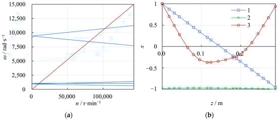
Figure 3. Analysis of critical speed and vibration mode of rotor: (a) Campbell diagram; (b) rotor vibration mode diagram.

Figure 3b shows the vibration modes corresponding to the first three critical speeds of the rotor. The first mode is conical, the second mode is cylindrical, and the third mode is curved. This indicates that the first two modes are rigid modes, in which the critical speed is caused by the low stiffness of the bearing, and the rotor can be considered a rigid body. The third mode is a bending mode, in which the critical speed is caused by the bending of the rotor, and the rotor can be considered a flexible rotor. Due to the low speed of the rigid mode, the bending mode is generally the focus of investigation.

Due to the bending critical speed of the rotor being 102,385 rpm, which is very close to the rated speed of the motor, the amplitude of vibration of the motor at the rated speed is very large. It is necessary to change the rotor parameters to increase the critical speed of the rotor. Generally, the measures to increase the bending critical speed of the rotor include increasing the diameter of the rotor and reducing the length of the rotor. The following discusses the relationship between increasing the diameter of each part and reducing the length and critical speed.

Figure 4a shows the effect of the diameter of the bearing section on the critical speed. It can be seen from the figure that the diameter of this section has little effect on the first to second order critical speeds. As the diameter increases, the third order critical speed increases significantly. When the diameter reaches 30 mm, the critical speed exceeds 140,000 rpm, with a high stability margin. Therefore, it is appropriate to use a diameter of 30 mm for this section.

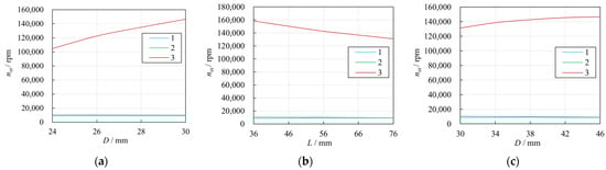
Figure 4. Bending patterns of the rotor at different rotational speeds: (a) diameter of bearing section; (b) length of permanent magnet; (c) outer diameter of rotor core.

Figure 4b shows the effect of the armature length on the critical speed. It can be seen from the figure that this parameter has little effect on the first and second order critical speeds. As the length increases, the third order critical speed decreases due to the increase in rotor length directly increasing the length of the rotor, thereby reducing the critical speed. Within the allowable range of electromagnetic force, this distance should be shortened as much as possible. Considering the balance of electromagnetic force and critical speed, a length of between 40 mm and 56 mm is appropriate.

Figure 4c shows the effect of the outer diameter ($D$) of the rotor iron core on the critical speed. It can be seen from the figure that this diameter has little effect on the first and second order critical speeds. As the inner diameter increases, the third order critical speed increases. When the diameter is greater than 38 mm, the increase in critical speed slows down. Therefore, $D$ is selected to be no less than 38 mm.

Based on the rotor dynamic optimization results, further optimization of motor electromagnetic performance can require an armature length ($L_{ef}$) of ≤56 mm and a rotor iron core outer diameter ($D$) of ≥38 mm.

3.3. Rotor Strength Analysis

Due to the material characteristics of permanent magnets, they can withstand large compressive stresses but cannot withstand large tensile stresses. Therefore, a protective sleeve is usually added around the permanent magnet to provide a radial preload between the sleeve and permanent magnet to compensate for tensile stresses generated by centrifugal forces during high-speed rotation.

The calculation method for tensile stress and compressive stress in permanent magnets can be analyzed through elastic mechanics theory or calculated using finite element method. Since there is little deviation between theoretical solutions and finite element solutions, simplified calculations are used in this paper for analysis.

Firstly, we analyzed the influence of $D$ on stress distribution in permanent magnets. By rotor dynamic analysis, it can be known that when $D$ ≥ 38 mm, take an inner diameter range of 38–50 mm. Then, take permanent magnet thickness as 1 mm, $h_{Sleeve}$ as 2 mm, and interference fit between permanent magnet and protective sleeve as 0.1 mm. The stress distribution includes static stress distribution after assembly and stress distribution during rotation considering the limit condition of the motor overspeed operation at $n=\mathrm{120,000}\mathrm{r}\mathrm{p}\mathrm{m}$.

Figure 5a shows the radial stress distribution in permanent magnets under a static state, where stress symbols with negative values represent compressive stress. It can be seen that compressive stress gradually increases from inside to outside along the direction of permanent magnet thickness. As the shaft diameter increases, the compressive stress decreases. Figure 5b shows the tangential stress distribution in permanent magnets under a static state, where stress slightly decreases from the inside diameter to the outside diameter along the direction of permanent magnet thickness. As the shaft diameter increases, compressive stress decreases.

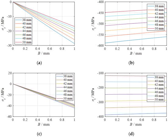
Figure 5. Stress distribution along the thickness direction of permanent magnets under different rotor core outer diameter conditions: (a) static radial stress; (b) static tangential stress; (c) dynamic radial stress; (d) dynamic tangential stress.

Figure 5c shows the radial stress distribution in permanent magnets under a dynamic state, where radial pressure is slightly higher than static pressure. Figure 5d shows the tangential stress distribution in permanent magnets under a dynamic state, where tangential pressure is significantly lower than static pressure and decreases more obviously with increasing $D$, which may be related to the higher centrifugal force influence with larger $D$.

Typically, permanent magnets can withstand a maximum compressive stress limit of about 1000 MPa and a maximum tensile stress limit of about 80 MPa. Therefore, under these conditions, when $D$ is within the range of 38–50 mm, stress distribution meets strength requirements.

Taking $D$ as 40 mm and other conditions as unchanged, analyze the influence of $h_{Nd}$ on stress. The range of $h_{Nd}$ is 1–4 mm.

Figure 6a shows the radial stress distribution of permanent magnets in a static state. With the increase in $h_{Nd}$, the radial compressive stress decreases. Figure 6b shows the tangential stress distribution of permanent magnets in a static state. With the increase in $h_{Nd}$, the tangential compressive stress decreases.

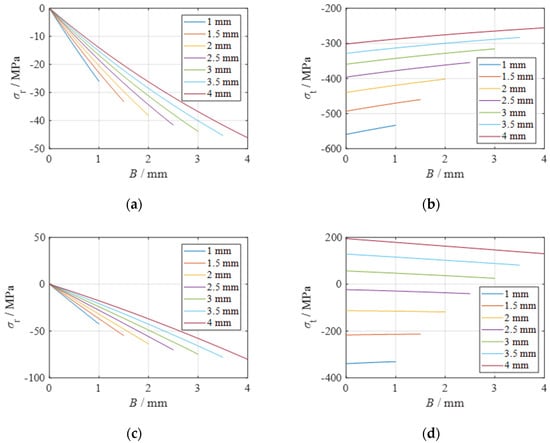
Figure 6. Stress distribution along the thickness direction of permanent magnets under different thickness conditions of permanent magnets: (a) static radial stress; (b) static tangential stress; (c) dynamic radial stress; (d) dynamic tangential stress.

Figure 6c shows the radial stress distribution of permanent magnets in a dynamic state, and the radial pressure is somewhat higher than that in a static state. Figure 6d shows the tangential stress distribution of permanent magnets in a dynamic state, and the tangential pressure is significantly lower than that in a static state. With the increase in $h_{Nd}$, the compressive stress gradually becomes tensile stress. When $h_{Nd}$ is greater than or equal to 3.5 mm, the tensile stress exceeds the tensile limit, and the permanent magnet is damaged.

It can be seen that the increase in $h_{Nd}$ will cause the tensile stress of permanent magnets to exceed the tensile limit and should be limited.

Taking $h_{Nd}$ as 1 mm and other conditions as unchanged, analyze the influence of $h_{Sleeve}$ on stress. The range of $h_{Sleeve}$ is 1–4 mm.

Figure 7a shows the radial stress distribution of permanent magnets in a static state with the increase in $h_{Sleeve}$. The radial compressive stress increases. Figure 7b shows the tangential stress distribution of permanent magnets in a static state with the increase in $h_{Sleeve}$. The tangential compressive stress increases. It can be seen that increasing $h_{Sleeve}$ can help increase the preload force.

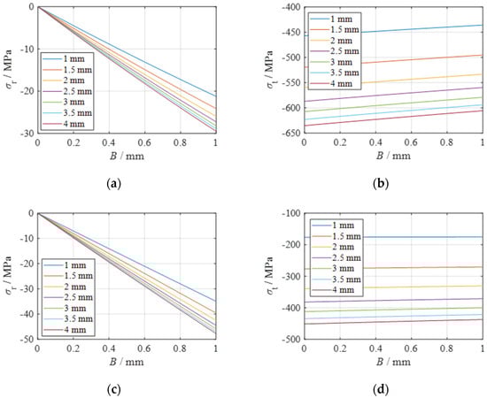
Figure 7. Stress distribution along the thickness direction of permanent magnets under different sleeve thickness conditions: (a) static radial stress; (b) static tangential stress; (c) dynamic radial stress; (d) dynamic tangential stress.

Figure 7c shows the radial stress distribution of permanent magnets in a dynamic state, and the radial pressure is somewhat higher than that in a static state. Figure 7d shows the tangential stress distribution of permanent magnets in a dynamic state, and the tangential pressure is significantly lower than that in a static state. With the increase in $h_{Sleeve}$, the amplitude of change in compressive stress is significantly reduced.

It can be seen that increasing $h_{Sleeve}$ can increase the preload force and reduce the difference between dynamic shear stress and static shear stress, preventing damage to the permanent magnet under dynamic conditions.

Taking $h_{Sleeve}$ as 2 mm and other conditions as unchanged, analyze the influence of interference on stress between permanent magnet and shaft with a range of interference as 0.05–0.2 mm.

Figure 8a shows the radial stress distribution of permanent magnets in a static state with the increase in interference. The radial compressive stress increases. Figure 8b shows the tangential stress distribution of permanent magnets in a static state with the increase in interference. The tangential compressive stress increases significantly. It can be seen that increasing interference can help increase preload force. It should be noted that when interference is greater than or equal to 0.175 mm, the compressive stress exceeds the compression limit of the permanent magnet, resulting in damage to it.

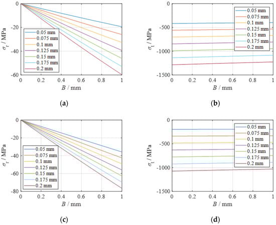
Figure 8. Stress distribution along the thickness direction of permanent magnets under different interference conditions: (a) static radial stress; (b) static tangential stress; (c) dynamic radial stress; (d) dynamic tangential stress.

Figure 8c shows the radial stress distribution of permanent magnets in a dynamic state with an increase in interference, and the radial pressure is somewhat higher than that in a static state. Figure 8d shows the tangential stress distribution of permanent magnets in a dynamic state with an increase in interference, and the tangential pressure is significantly lower than that in a static state.

It can be seen that increasing interference can significantly increase preload force and prevent damage to the permanent magnet under dynamic conditions, but it should be noted that too large a static compressive stress can cause damage to permanent magnets.

Based on the above analysis, it can be concluded that an increase in $D$ will increase centrifugal force-induced tensile stress; an increase in $h_{Nd}$ will significantly increase high-speed tensile stress and cause damage to permanent magnets; an increase in $h_{Sleeve}$ can reduce high-speed centrifugal force on permanent magnet stress; an increase in interference can significantly increase preload compressive stress.

Through calculations, we give limiting conditions as follows:

$$s.t.\left\{\begin{array}{c}38\le D\le 42\\ 1\le h_{Nd}\le 2\\ 2\le h_{Sleeve}\le 3\\ 40\le L_{ef}\le 56\end{array}\right.$$

(2)

The above stress limits meet the strength requirements of the permanent magnet, so the motor performance can be further optimized within this range.

4. Coupled Modeling and Analysis of Electromagnetic Field and Temperature Field in Electric Motors

4.1. Finite Element Modeling of Electromagnetic Fields

The finite element modeling of the ultra-high-speed motor is described in reference [48]. Considering the symmetry of the motor, a two-dimensional model is adopted to reduce computational complexity. The model uses a potential function to solve both the magnetic vector potential $\mathit{A}$ and the magnetic scalar potential $\mathit{\varphi }$.

Once the electromagnetic field problem is solved, the magnetic vector $\mathit{A}$ can be determined, which allows for the derivation of the performance parameters for the motor. Figure 9 displays the magnetic field distribution of the motor’s finite element model under no-load conditions.

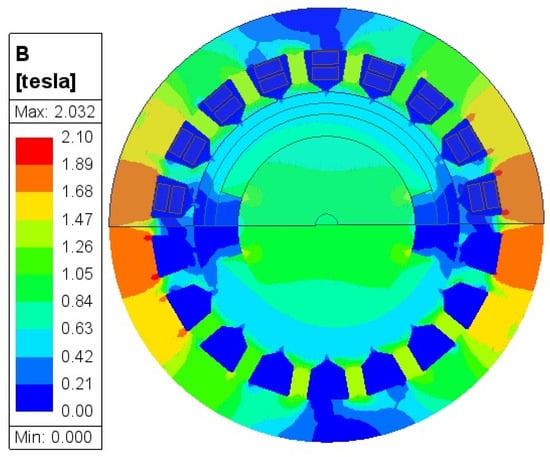
Figure 9. Diagram of radial magnetization.

4.2. Finite Element Modeling of Temperature Field

The ultra-high-speed motor adopts water cooling. The basic assumptions for fluid flow and heat transfer calculations in various regions of the motor are as follows:

(1)

Basic assumptions and boundary conditions for fluid flow and thermal coupling calculations in electric machines.

(2)

Assuming that the upper and lower stator windings are of the same width.

(3)

It is believed that the components in the motor are in close contact and have no contact thermal resistance.

(4)

Assuming that the heat of the motor is only removed by convection through the fluid in the cooling water jacket, and that there is no heat transfer between the motor and the air.

(5)

Ignoring the influence of heat dissipation at the end of the stator.

(6)

Due to the high Reynolds number of the fluid inside the water jacket, the flow belongs to turbulent flow. A turbulence model is adopted for the fluid and solved; the fluid is incompressible.

Based on the above assumptions, the boundary conditions for the calculation model in this article are as follows:

(1)

Since the fluid in the water jacket is incompressible, the rated water velocity is 20 L/min, and the inlet temperature is 40 °C.

(2)

The ambient temperature of the motor is set to 25 °C.

(3)

All solid surfaces are set as wall boundary conditions, and coupling is added between surfaces to allow temperature transfer.

(4)

The heat sources in the motor include the stator teeth, the stator yoke, and the stator winding.

Figure 10 is a mesh division diagram of the finite element model of heat transfer of the motor. The division quality is good and can meet the following temperature field calculation.

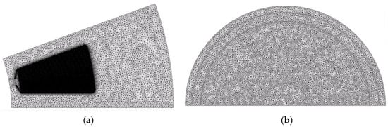
Figure 10. Motor grid subdivision: (a) stator slot; (b) rotor.

In order to obtain the temperature distribution in the medium, it is necessary to solve the heat flow equation in an appropriate form. However, this solution depends on the physical conditions at the boundary of the medium. If the process changes with time, this solution also depends on the internal conditions of the medium at a certain starting time. When it comes to boundary conditions, there are several common physical effects at the boundary, which can be simply expressed in mathematical formulas. In order to determine the temperature distribution inside the object, for the above heat conduction equation, it is necessary to give appropriate boundary conditions. Common boundary conditions are divided into three categories.

(1)

Temperature boundary conditions (first type of boundary condition):

$$\left\{\begin{array}{c}T\left(x,y,z\right){|}_{S_1}=T_C\\ T\left(x,y,z\right){|}_{S_1}=f\left(x,y,z,t\right)\end{array}\right.$$

(3)

where $T_c$ is the given temperature on the boundary surface $S_1$, $f\left(x,y,z,t\right)$ is a known temperature function, and $S_1$ is the object boundary.

(2)

The boundary condition for heat flow (second type of boundary condition):

$$\left\{\begin{array}{c}-\lambda {\displaystyle \frac{\partial T}{\partial n}}{|}_{S_2}=q_0\\ -\lambda {\displaystyle \frac{\partial T}{\partial n}}{|}_{S_2}=g\left(x,y,z,t\right)\end{array}\right.$$

(4)

where the heat conduction at the boundary is a known value $q_0$ (outward) and refers to the known normal gradient of the boundary. When $q_0=0$, there is no heat conduction on this surface, which is called an adiabatic boundary condition.

In this equation, $q_0$ represents the boundary heat flow input on the $S_2$ surface, $\mathrm{g}\left(x,y,z,t\right)$ is the heat flow density function, and $\mathsf{\lambda }$ is the coefficient of heat conduction perpendicular to the surface of the object.

(3)

Thermal exchange boundary condition (third type of boundary condition):

The heat flow rate transmitted from the interior of the object to the boundary on boundary $S_3$ is equal to the heat flow rate dissipated into the surrounding medium through this boundary. This equation is shown below:

$$-\lambda {\displaystyle \frac{\partial T}{\partial n}}{|}_{S_3}=\mathsf{\alpha }\left(T-T_0\right)$$

(5)

where $T_0$ represents the temperature of the surrounding medium, $\mathsf{\alpha }$ is the heat transfer coefficient of the $S_3$ surface, and both $T_0$ and $\mathsf{\alpha }$ can be constants or functions of time and position.

When using the finite element method to calculate temperature rise in an ultra-high-speed motor, determining the physical parameters of the model is crucial. Physical properties are all reflected by material properties, so the material must be assigned to each entity. When conducting temperature field analysis, motor materials include parameters such as density, specific heat capacity, and coefficient of heat conduction. The main components in this analysis involve permanent magnets, non-magnetic alloy steel, stator steel laminations, copper windings, insulation, the casing, and so on. Table 4 are some material property values:

Table 4. Data sheet of materials used in the model.

Name	Material	Density (kg/m3)	Thermal Conductivity (W/m °C)	Specific Heat Capacity (J/kg °C)
Core	Silicon steel sheets	7800	42.5	502.4
Winding	Copper	8900	387.6	504
Air inside the air gap	Air	1.18	0.026	1042
Permanent magnet protective sleeve	Carbon fiber	1600	0.59	1000
PM	NdFeB	8400	8	504
Axle	Steel	7800	50	504
Housing	Aluminum alloy	2790	168	833
Slot insulation	Polyimide	1430	0.35	1130

The losses in the motor thermal circuit model are calculated using an electromagnetic model. When the motor speed is 100,000 r/min and the DC bus voltage is 540 V with a peak phase current of 35 A, the electromagnetic model calculates the iron loss distribution shown in Figure 11. It can be seen that the iron loss mainly occurs around the stator slots, while the rotor loss mainly occurs on the surface of the permanent magnets and iron core. The loss distribution values are shown in Table 5. These losses are directly imported into the motor thermal field model for temperature field simulation calculations.

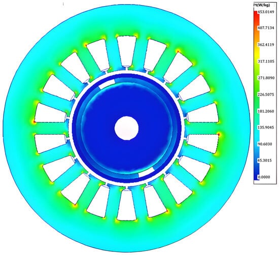
Figure 11. Cloud chart of motor loss distribution.

Table 5. Distribution value of motor loss.

Component	Loss (W)
Stator yoke	248.4
Stator teeth	87.97
Rotor yoke	3.224
PM	3.632
Winding	144.3

Figure 12 shows the temperature distribution of the motor calculated using finite element analysis. The high-temperature area is mainly concentrated in the stator winding, with a maximum temperature of no more than $130°\mathrm{C}$, and a maximum temperature of no more than $120°\mathrm{C}$ in the rotor area.

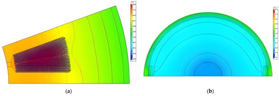
Figure 12. Cloud diagram of temperature distribution obtained through finite element calculation: (a) stator; (b) rotor.

4.3. Coupling Model of Electromagnetic and Temperature

According to the analysis, motor loss is the direct factor causing motor heating, which in turn affects the distribution of the motor temperature field. The temperature directly affects the change in internal resistance of the armature winding, and its resistivity can be expressed by Formula (6).

$$\rho \left(T\right)={\rho }_0\left(1+\alpha \left(T-T_0\right)\right)$$

(6)

where $\rho \left(T\right)$ is the resistivity at temperature $T$, ${\rho }_0$ is the resistivity at temperature $T_0$, and $\alpha$ is the temperature coefficient.

Meanwhile, temperature also affects the residual magnetic density of permanent magnets, thereby reducing the air gap magnetic field of the motor.

Therefore, in the actual model calculation process, the coupling relationship between electromagnetic field and temperature field must be considered to ensure accurate calculation. Based on the electromagnetic field and temperature field models, a coupled model is established with motor losses and temperature as transfer parameters between the two physical fields.

Table 6 compares the electromagnetic performance of two models. It can be seen that due to the consideration of the coupling relationship between thermal and electromagnetic fields, the output power calculated by the coupled model is smaller than that of the non-coupled model, and the efficiency is also lower. The main reason is that under load, the actual temperature of the motor will increase. In this case, the temperature of the permanent magnet reached 108.6 °C, and the temperature of the armature conductor reached 122.2 °C, instead of the fixed value of 40 °C given by the uncoupled model, resulting in a decrease in residual magnetism of the permanent magnet from 1.279 T to 1.171 T. The comparison of the magnetic field cloud map of the motor model is shown in Figure 13, and the air gap magnetic density decreased from 0.5608 T to 0.5213 T. Therefore, under the same current conditions, the power decreases. At the same time, due to the increase in winding temperature (122.2 °C), the phase resistance also increased from the original 0.05814 Ω to 0.07527 Ω, resulting in an increase in about 30 W in copper loss. Although the stator iron loss decreased by 50 W due to the decrease in magnetic density, the total output power of the motor decreased by nearly 1.2 kW, leading to a decrease in overall motor efficiency. It can be seen that the results calculated using the electromagnetic field thermal field coupling model are more realistic and have higher accuracy.

Table 6. Comparison of electromagnetic performance between two models.

Name	Coupled Model	Decoupled Model
Output power (W)	13,509	14,735
Air gap magnetic density (amplitude) (T)	0.5213	0.5608
Residual magnetization of permanent magnet (T)	1.171	1.279
Efficiency (%)	96.609	96.765
Phase resistance (Ω)	0.07527	0.05814
Armature DC copper loss (W)	138.3	106.8
Stator core loss (W)	329	379
Armature conductor temperature (°C)	122.2	40
Rotor temperature (°C)	107.5	40

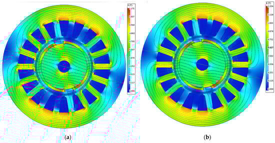
Figure 13. Electromagnetic field cloud map: (a) coupling model of electromagnetic and thermal effects; (b) electromagnetic model.

5. Coupling Model Based on Mechanical Field Limitations

5.1. Coupling Modeling

Considering that the deformation caused by the force on the motor structure is very small and has little effect on the electromagnetic field, the main consideration is the dynamic characteristics of the motor rotor at high speeds.

Therefore, the design of the motor rotor follows the following principles:

(1)

Determine the limit value of the outer radius of the permanent magnet based on the surface speed requirements of the rotor.

(2)

According to the strength requirements of the rotor, determine the thickness of the protective sleeve $h_{sleeve}$ and the interference amount ${\delta }_s$ restriction.

(3)

Determine the outer rotor diameter and axial length limit values based on the stiffness and critical speed of the rotor.

Then, the size limit value is used as a constraint condition for the optimization design model, and a multi-physics field coupling optimization model for the motor is established, as shown in Figure 14.

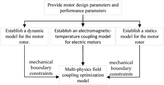
Figure 14. Coupling model of electromagnetic field and temperature field.

5.2. Parametric Design of Coupled Models

In order to optimize the design of the motor, the established coupling model was parameterized and the range of parameter values was determined based on the previous analysis. The specific design parameters include the following: cooling system parameters ($h_{\mathrm{d}\mathrm{u}\mathrm{c}\mathrm{t}}$, $h_{\mathrm{J}\mathrm{a}\mathrm{c}\mathrm{k}\mathrm{e}\mathrm{t}}$, $b_{duct}$), overall dimensions of the motor ($D_{o1}$, $D$, $L_{ef}$, $h_{Sleeve}$, $L_{Airgap}$), permanent magnet parameters ($h_{Nd}$, $b_{embrace}$), internal parameters of the stator ($bs0$, $h_{tooth}$, $hs0$, $Ang$, $hs2$, $r1$), as shown in Figure 15, and winding parameters ($Nstrands$, $I_{phase}$). Dimensional limitations are imposed on the outer diameter of the rotor core, armature length, and sleeve thickness based on mechanical properties, as shown in Equation (2).

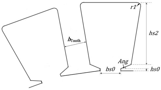
Figure 15. Coupling model of electromagnetic field and temperature field.

As shown in Table 7, the main performance parameters of the motor are as follows: motor efficiency ($\eta$), output power ($P_{out}$), cogging torque ($T_{cog}$), maximum winding temperature ($T_{coilMax}$), and power density ($k_p$).

Table 7. Optimize the range of design parameters.

	Name	Variable	Unit	Range
Cooling system parameters	Sink height	hduct	mm	2–10
	Wall thickness of water jacket	hJacket	mm	1–3
	Sink span	bduct	mm	6–12
	Coolant flow rate	v0	L/min
Overall dimensions of motor	Outer diameter of stator	Do1	mm	110–130
	Outer diameter of rotor core	D	mm	38–42
	Armature length	Lef	mm	40–56
	Sleeve thickness	hSleeve	mm	1–3
	Air gap length	LAirgap	mm	0.3–1.5
PM parameters	Thickness of permanent magnet	hNd	mm	1–2
	Permanent magnet width	bembrace	°	140–180
Internal parameters of the stator	Slot opening	bs0	mm	1–4
	tooth width	htooth	mm	3–7
	Shoulder height of slot	hs0	mm	0.3–3
	Slot Shoulder angle	Ang	°	15–30
	slot depth	hs2	mm	12–18
	Radius of slot bottom corner	r1	mm	0.5–2
Winding parameters	Number of parallel windings	Nstrands		280–340
	Phase current	Iphase	A
Motor performance	Efficiency	η	%
	Output power	Pout	kW
	Cogging torque	Tcog	Nm
	Maximum temperature of winding	TcoilMax	°C
	Fill factor	ks	%
	Power density	kp	kW/kg

6. Optimized Design of High-Speed Motor

When dealing with the optimization of electric motors, numerous objectives and design parameters frequently arise. Nevertheless, establishing precise, explicit formulas linking these design parameters to the optimization objectives is often infeasible. Typically, the intricate relationship between them is derived through finite element simulation calculations, a process referred to as constructing a surrogate model, as illustrated in Figure 16.

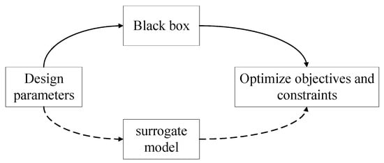
Figure 16. Schematic diagram of surrogate model.

6.1. Optimization Model

With the optimization objectives of maximizing efficiency and power density, while simultaneously limiting cogging torque, slot fill factor, maximum temperature rise of windings, and output power, the optimization model is presented in Equation (7), and the design parameters are shown in Equation (8). The range of values for each design parameter is illustrated in Table 7.

$$\begin{array}{c}\max y=\left\{\begin{array}{cc}\eta \left(x\right),& k_p\left(x\right)\end{array}\right\}\\ s.t.\left\{\begin{array}{c}{T}_{cog}\left(x\right)\le 0.00015\\ k_s\le 0.8\\ T_{coilMax}\le 140\\ 14000\ge P_{out}\ge 12000\\ x_i^1\le x_i\le x_i^2\end{array}\right.\end{array}$$

(7)

$$x=\left\{\begin{array}{c}bs0,b_{embrace},L_{Airgap},h_{Nd},h_{Sleeve},L_{ef},D_{O1},\\ h_{tooth},D,I_{Phase},h_{Jacket},Nstrands,hs0,hs2\end{array}\right\}$$

(8)

6.2. Optimization Process

Based on the ultra-high-speed motor model that couples electromagnetic and thermal fields, an optimization design algorithm based on a surrogate model is adopted to optimize the design of the ultra-high-speed motor. The specific optimization process is shown in Figure 17. Firstly, the electromagnetic-thermal coupling model is used to conduct a sensitivity analysis of the motor, providing parameters for motor optimization design. At the same time, constraints on motor design parameters are given based on the analysis of the motor’s mechanical field. Then, an optimization design model based on multi-physical field coupling is established. A MaxPro experimental design is used to obtain initial samples. After calculation using the multi-physical field coupling model, a surrogate model is fitted using Kriging. Based on this surrogate model, genetic algorithms are used for optimization design, and the optimization results are verified. If the requirements are not met, new samples are added to rebuild a new Kriging surrogate model and perform optimization design until the accuracy is met.

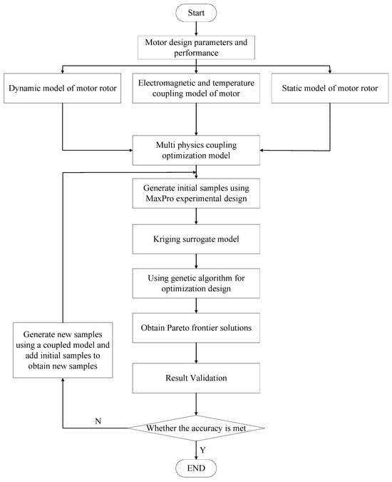
Figure 17. Optimization design process based on multi-physical field coupling.

6.2.1. Experimental Design

In 2015, Joseph, Gul, and Ba introduced a Maximum Projection (MaxPro) experimental design that incorporates a weight factor to guarantee accurate predictions across all subspaces [49]. The underlying concept is outlined as follows:

$$\underset{D}{\min }\sum _{i=1}^{n-1}\sum _{j=i+1}^n{\displaystyle \frac{1}{d^k\left(x_i,x_j;w\right)}}p\left(w\right)dw$$

(9)

$$d\left(x_i,x_j;w\right)={\left({\sum }_{l=1}^p{\mathrm{w}}_{\mathrm{i}\mathrm{l}}{\left|{\mathrm{x}}_{\mathrm{i}\mathrm{l}}-{\mathrm{x}}_{\mathrm{j}\mathrm{l}}\right|}^{\mathrm{s}}\right)}^{1/\mathrm{s}}$$

(10)

where $\mathrm{w}=\left({\mathrm{w}}_1,\cdots ,w_p\right)$, ${\sum }_{l=1}^p{w}_l=1$, $w_1,\cdots w_l>0$, $w_l$ is the weight, and $p\left(w\right)$ represents the priority distribution factor of the weight. When $w$ is uniformly distributed and $w=s\times p$, Formula (9) can be simplified to Formula (11), where $s$ is typically set to 2.

$$d \underset{D}{\min }\sum _{i=1}^{n-1}\sum _{j=i+1}^n{\displaystyle \frac{1}{{\prod }_{l=1}^p{\left|x_{il}-x_{jl}\right|}^s}}$$

(11)

The MaxPro experimental design does not rely on an even spacing distribution; instead, it aims to reach the boundaries as extensively as possible, making it exceptionally well-suited for surrogate models with a high number of dimensions.

Figure 18 depicts the partial factor distribution of the initial 500 samples acquired through the MaxPro experimental design. It illustrates that the samples are spread uniformly across the entire design space, ensuring comprehensive coverage.

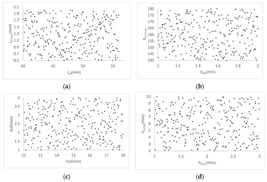
Figure 18. Partial factor distribution: (a) $L_{\mathrm{A}\mathrm{i}\mathrm{r}\mathrm{g}\mathrm{p}}$ vs. $L_{\mathrm{e}\mathrm{f}}$; (b) $b_{\mathrm{e}\mathrm{m}\mathrm{b}\mathrm{r}ace}$ vs. $h_{Nd}$; (c) bs0 vs. hs2; (d) $h_{\mathrm{J}acket}$ vs. $h_{\mathrm{d}\mathrm{u}\mathrm{c}\mathrm{t}}$.

6.2.2. Kriging Surrogate Model

The Kriging model, illustrated in Equation (12), integrates a global model with local deviations. Due to its exceptional global approximation and error estimation abilities, it is particularly well-suited for addressing nonlinear problems [50].

$$y\left(x\right)=f\left(x\right)+\mathrm{z}\left(x\right)$$

(12)

where $x$ represents the design parameter, $y\left(x\right)$ denotes the response function, $f\left(x\right)$ employs a global approximation model of polynomial response surface, and $z\left(x\right)$ signifies local error.

Among them, $z\left(x\right)$ represents a static Gaussian random process with an expected value of 0 and a variance of ${\sigma }^2$. The covariance is shown in (13).

$$\mathrm{C}\mathrm{o}\mathrm{v}\left[z\left(x_i\right),z\left(x_j\right)\right]={\sigma }^2\mathit{R}\left[R\left(x_i,x_j\right)\right]$$

(13)

where $\mathit{R}$ represents the correlation matrix, and $R\left(x_i,x_j\right)$ denotes the correlation function between two samples.

Use the Gaussian correlation function, as shown in Equation (14):

$$R\left(x_i,x_j\right)=\mathrm{e}\mathrm{x}\mathrm{p}\left(-\sum _{k=1}^m{\theta }_k\left|x_{ik}-x_{jk}\right|\right)$$

(14)

where $m$ represents the number of design parameters, and ${\theta }_k$ denotes the unknown correlation coefficient used for fitting the approximate model.

The estimated value at $x$ is as follows:

$$\widehat{y}=\widehat{\beta }+r^T\left(x\right){\mathit{R}}^{-1}\left(y-\mathbf{f}\widehat{\beta }\right)$$

(15)

where $\mathbf{f}$ represents a unit column vector of length $n$, $y$ denotes the response column vector of $n$ sample points, and $r^T\left(x\right)$ signifies the correlation vector between the $n$ sample points and $x$. Among them

$$r\left(x\right)=\left[R\left(x,x_1\right),R\left(x,x_2\right),\cdots R\left(x,x_n\right)\right]$$

(16)

$$\widehat{\beta }={\left({\mathbf{f}}^T{\mathit{R}}^{-1}\mathbf{f}\right)}^{-1}{\mathbf{f}}^T{\mathit{R}}^{-1}\mathrm{y}$$

(17)

The estimated variance is

$${\widehat{\sigma }}^2={\displaystyle \frac{\left(y-\mathbf{f}\widehat{\beta }\right){\mathit{R}}^{-1}\left(y-\mathbf{f}\widehat{\beta }\right)}{n}}$$

(18)

The maximum likelihood estimation used for the Kriging model is

$$\mathrm{m}\mathrm{a}\mathrm{x}\mathsf{\Phi }\left({\theta }_k\right)={\displaystyle \frac{n\mathrm{l}\mathrm{n}\left({\widehat{\sigma }}^2\right)+\mathrm{l}\mathrm{n}\left|\mathit{R}\right|}{2}}$$

(19)

The Kriging approximation model is obtained by solving the unconstrained optimization problem using numerical optimization algorithms.

Establish a Kriging surrogate model that maps design parameters to motor performance, as shown in Equation (20):

$$\left\{\begin{array}{c}x=\left\{\begin{array}{c}bs0,b_{embrace},L_{Airgap},h_{Nd},h_{Sleeve},L_{ef},D_{o1,}\\ h_{tooth},D,I_{Phase},h_{Jacket},Nstrands,hs0,hs2\end{array}\right\}\\ \left[k_p,k_s,\eta ,P_{out},T_{cog},T_{coilMax}\right]=F\left(x\right)\end{array}\right.$$

(20)

Relative Maximum Absolute Error (RMAE) and Relative Average Absolute Error (RAAE) are adopted as evaluation metrics for the optimization model. The calculation formulas for RAAE and RMAE are shown in Equations (21) and (22), respectively.

$$\mathrm{R}\mathrm{A}\mathrm{A}\mathrm{E}={\displaystyle \frac{\frac{1}{N}\sum _{i=1}^N\left|y_i-{\widehat{y}}_i\right|}{\sqrt{\frac{1}{N-1}\sum _{i=1}^N{\left(y_i-{\widehat{y}}_i\right)}^2}}}$$

(21)

$$\mathrm{R}\mathrm{M}\mathrm{A}\mathrm{E}={\displaystyle \frac{\frac{1}{N}\underset{i=1:N}{\mathit{max}}\left(\left|y_i-{\widehat{y}}_i\right|\right)}{\sqrt{\frac{1}{N-1}\sum _{i=1}^N{\left(y_i-{\widehat{y}}_i\right)}^2}}}$$

(22)

where $N$ represents the number of test points, $y_i$ denotes the true value of the ith test point, and ${\widehat{y}}_i$ signifies the predicted value of the ith test point.

RMAE and RAAE serve as metrics to assess the local and global precision of the model, respectively. Lower values indicate higher model accuracy.

Figure 19 displays partial outcomes from fitting the Kriging surrogate model. While the surrogate model generally captures the global traits of the samples, its local prediction accuracy is moderate, as depicted in Figure 20. Specifically, the RAAE is below 1 and the RMAE is close to 0. Hence, during the optimization design process, it is crucial to conduct adaptive iterations on the samples to enhance accuracy.

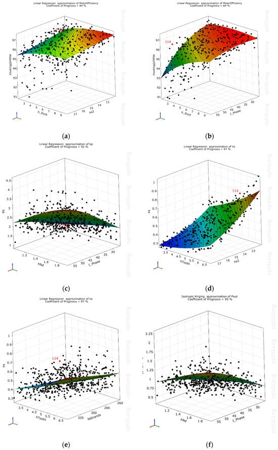
Figure 19. Partial fitting surface of Kriging model: (a) $\eta \mathrm{v}\mathrm{s}. h_{Duct}$, $h_{s2}$; (b) $\eta \mathrm{v}\mathrm{s}. h_{Duct}$, $I_{Phase}$; (c) $k_P \mathrm{v}\mathrm{s}. h_{Nd}$, $I_{Phase}$; (d) $k_s \mathrm{v}\mathrm{s}. h_{Tooth}$, $h_{s2}$; (e) $k_s \mathrm{v}\mathrm{s}. h_{Tooth}$, $NStands$; (f) $P_{out} \mathrm{v}\mathrm{s}.h_{Nd}$, $I_{Phase}.$

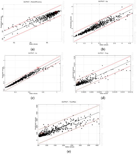
Figure 20. Prediction accuracy: (a) RAAE and RMAE of $\eta$ are 0.692, 0.0085; (b) RAAE and RMAE of $k_p$ are 0.731, 0.01; (c) RAAE and RMAE of $k_s$ = 0.707 = 0.011; (d) RAAE and RMAE of $T_{cog}$ are 0.587, 0.011; (e) RAAE and RMAE of $T_{coilMax}$ are 0.638, 0.01.

6.2.3. NSGA-2

The schematic diagram of the NSGA-2 algorithm is shown in Figure 21 [51]. Its main features are as follows: using fast sorting based on Pareto dominance level can quickly calibrate the dominance level of each individual in the population, and using crowding distance instead of the fitness sharing mechanism can obtain a uniformly distributed Pareto optimal solution set. At the same time, using an elite retention mechanism can make it easier to obtain excellent next generations. Among them, the crowding distance, as shown in Equation (23), is the average value of the Euclidean distance.

$$PCD\left(p_k\right)={\displaystyle \frac{1}{m}}{\displaystyle \sum \frac{f_i\left(p_{k+1}\right)-f_i\left(p_{k-1}\right)}{f_i^{max}-f_i^{min}}}$$

(23)

where $f\left(p_{k+1}\right)$, $f\left(p_k\right)$, and $f\left(p_{k-1}\right)$ are three consecutive Pareto front points and $p_{k+1}$, $p_k$, $p_{k-1}$ are the corresponding Pareto solutions; $f_i^{min}$, $f_i^{max}$ are the minimum and maximum values of the $i^{th}$ objective function of the Pareto front, respectively.

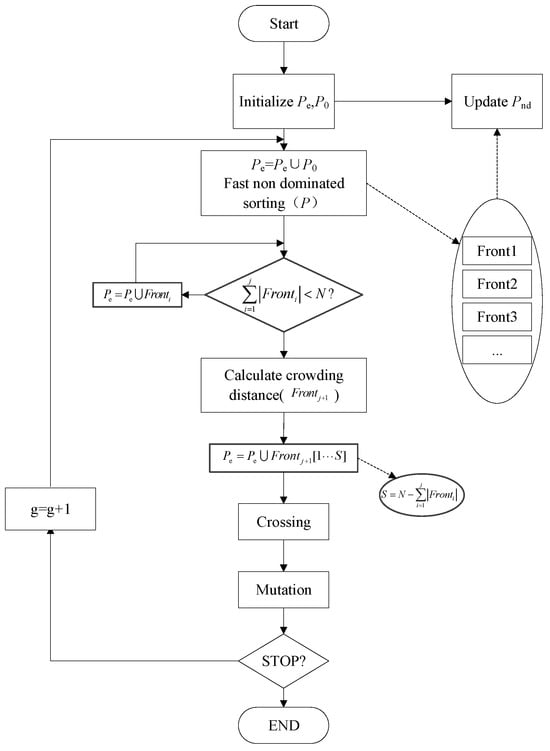
Figure 21. NSGA-2.

6.2.4. Optimization Result Analysis

The MaxPro design is utilized to obtain an initial set of 500 samples. The number of correction points amounts to 50, while there are 200 non-dominant solutions considered. The process involves 500 iterations, and the convergence criteria have been set as

$$\left\{\begin{array}{c}\mathrm{RMAE}\le 0.01\\ \mathrm{RAAE}\le 0.1\end{array}\right.$$

(24)

Figure 22 shows that the RMAE and RAAE of the output parameters are less than 0.01 and 0.1 at the fifth generation, and the samples are only 750.

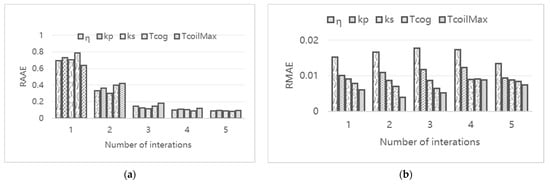
Figure 22. Convergence process: (a) RAAE; (b) RMAE.

Figure 23 shows the optimized Pareto front, as indicated by the red line in the figure. In this project, five schemes were selected from the Pareto front according to different requirements, as shown in Table 8. The performance parameters achieved the optimization design goals, with efficiency reaching 97% and power density exceeding 4 kW/kg.

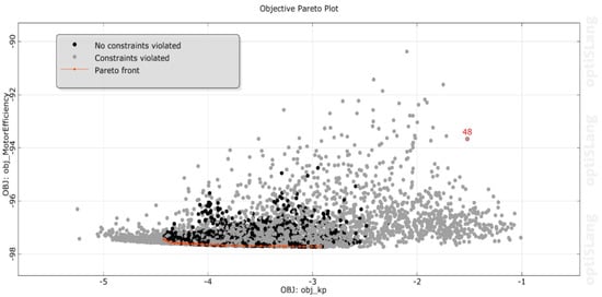
Figure 23. Pareto frontier.

Table 8. Performance and design parameters of five designs.

Parameter	Case1	Case2	Case3	Case4	Case5
hSleeve (mm)	2.17	2.20	2.13	2.12	2.17
NStrands	340	340	340	340	340
DO1 (mm)	110.24	110	130	110	116.6
hJacket (mm)	1.5	1.5	1.5	1.5	1.5
bduct (mm)	9	9	9	9	9
Lef (mm)	40	40	41.75	45.75	40
LAirgap (mm)	0.5	0.5	0.5	0.5	0.5
hDuct (mm)	10	8.19	10	8.98	9.98
bThrow (mm)	9	9	9	9	9
hNd (mm)	2	2	2	2	2
r1	1	1	1	1	1
bembrace (degree)	179.44	180	180	163.64	178.39
hs2 (mm)	14	14	14	14	14
bs0 (mm)	1.32	1	1.01	1.64	1.18
Ang (degree)	30	30	30	30	30
hs0 (mm)	0.625	0.719	0.774	0.85	0.68
hTooth (mm)	6.22	6.39	6.42	6.45	6.46
D (mm)	41.99	41.82	42	41.97	41.95
IPhase (A)	48.72	48.72	43.30	48.26	48.72
$\eta$ (%)	97.55	97.44	97.72	97.52	97.64
Pout (kW)	12,998.08	12,994.38	12,266.47	13,941.6	12,992.84
Tcog (N)	0.00269	0.00055	0.0005	0.0028	0.0027
TcoilMax (°C)	94.96	105.79	87.52	87.39	94.76
kp	4.349	4.423	3.983	4.406	4.006
ks	0.767	0.792	0.788	0.8	0.794

Then, finite element analysis was used to verify the accuracy of the five optimization schemes. The verification results are shown in Table 9. The efficiency error of the five optimization schemes is within 1%, and the power density error does not exceed 7%, which meets the requirements. Considering the efficiency and power density of the motor comprehensively, case 2 is chosen as the final design solution.

Table 9. Verification results.

Cases		η	kp
case1	Optimize design values	97.03	4.349
	Model calculation value	97.556	4.1
	error	0.54%	−6.07%
case2	Optimize design values	97.44	4.4232
	Model calculation value	96.95	4.23052
	error	−0.5%	−4.55%
case3	Optimize design values	97.72	3.983
	Model calculation value	96.99	4.18
	error	−0.74%	4.71%
case4	Optimize design values	97.52	4.41
	Model calculation value	97.133	4.27
	error	−0.39%	−3.28%
case5	Optimize design values	97.64	4.0
	Model calculation value	97.28	3.78
	error	−0.37%	−5.82%

6.3. Motor Performance

Simulation calculations were performed on the final design case with a working bus voltage of 540 V and sinusoidal drive. The final power MAP and efficiency MAP of the motor are shown in Figure 24 and Figure 25. The maximum motor speed is 150,000 r/min, and the highest efficiency reaches 97%, with over 90% accounting for over 80%.

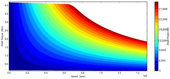
Figure 24. MAP of motor power.

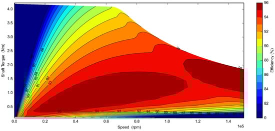
Figure 25. MAP of motor efficiency.

7. Experiments and Verification

Due to the inability to find testing equipment for this type of ultra-high-speed motor on the current market, this project plans to adopt a simplified testing scheme to indirectly complete motor performance testing, as shown in Figure 26. The measurement and control system sets the controller speed, and the controller controls the compressor to operate at the given speed. The measurement and control system measures the inlet and outlet pressures of the compressor to calculate the pressure ratio. The power consumption of the compressor is indirectly calculated through the pressure difference and flow rate according to Equation (25). At the same time, the measurement and control system needs to test the motor voltage and current to calculate the electric power ($P_e$). The motor efficiency is calculated according to Equation (26), where ${\eta }_c$ is the motor controller efficiency.

$$P_{Air}=∆\mathrm{p}\times v_{Air}\times {\displaystyle \frac{1}{{\eta }_{Air}}}$$

(25)

$${\eta }_{motor}={\displaystyle \frac{P_{Air}}{P_e}}\times {\displaystyle \frac{1}{{\eta }_c}}\times 100\mathrm{\%}$$

(26)

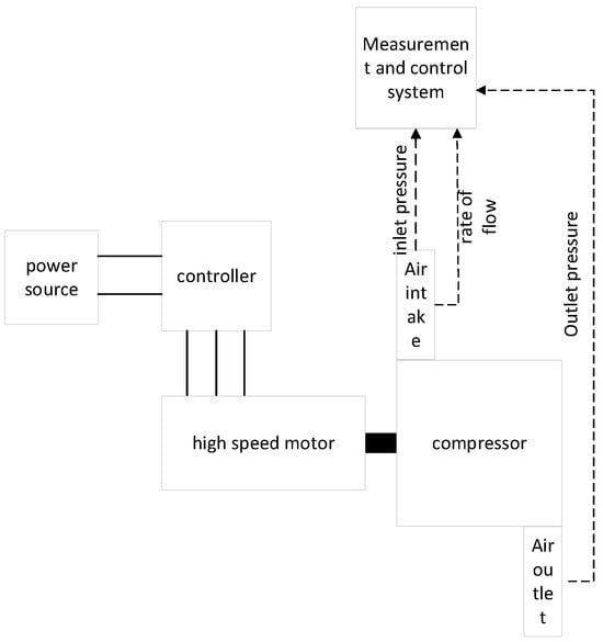
Figure 26. Principle block diagram of the test platform.

Table 10 shows the mass of each part of the two motors, designed according to a rated power of 12 kW, with a power density of 4 kW/kg.

Table 10. Motor power density.

Name	Weight
	JQHM-SZ22010001	JQHM-SZ22010002
Stator core (kg)	1.41	1.43
Rotor (kg)	0.56	0.53
PM (kg)	0.084	0.081
Winding (kg)	0.87	0.85
Total (kg)	2.924	2.911
Power density (kW/kg)	4.1	4.12

A testing platform was built according to Figure 26, as shown in Figure 27, and ultra-high-speed motor performance tests were conducted on both motors. During the test, the temperature was controlled at $20–35 °\mathrm{C}$, and the atmospheric pressure was controlled at $101 \mathrm{k}\mathrm{P}\mathrm{a}$.

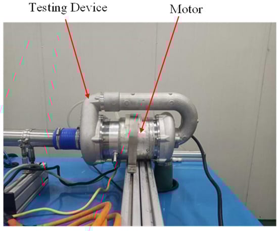
Figure 27. Motor testing bench.

The test data of the JQHM-SZ22010001 motor are shown in Table 11, and the test data of the JQHM-SZ22010002 motor are shown in Table 12. If the efficiency of the motor controller is estimated at 96%, the actual efficiency of the motor can be obtained. It can be seen that the efficiency of both motors can exceed 95% at around 12 kW, meeting the design specifications, and the efficiency is also close to 95% at 8 kW power.

Table 11. Experimental data of JQHM-SZ22010001.

Speed (r/min)	Inlet Water Temperature (°C)	Outlet Water Temperature (°C)	Air Compressor Pressure Ratio	Mass Flow (g/s)	Air Compressor Power Consumption (Kw)	Average Current (A)	Voltage (V)	Motor Temperature (°C)	Efficiency (%)
50,000	23.13	35.75	1.162	80.3	5.725	11.7	538	46	94.7
60,000	21.72	41.81	1.271	89.8	6.843	14.0	536	53	95
70,000	21.75	49.32	1.453	99.1	7.986	16.4	535	64	94.7
80,000	21.92	51.91	1.876	119.2	9.128	18.7	535	74	95.2
90,000	21.5	61.06	1.932	139.4	10.271	21.0	534	81	95.4
100,000	21.8	66.72	2.201	154.5	11.446	23.2	534	97	96.25

Table 12. Experimental data of JQHM-SZ22010002.

Speed (r/min)	Imported Water Temperature (°C)	Outlet Water Temperature (°C)	Air Compressor Pressure Ratio	Mass Flow (g/s)	Air Compressor Power Consumption (kW)	Average Current (A)	Voltage (V)	Motor Temperature (°C)	Efficiency (%)
50,000	22.19	36.14	1.153	79.8	5.736	11.7	539	48	94.7
60,000	21.9	44.47	1.266	90.6	6.866	14.0	537	56	95.1
70,000	21.81	56.74	1.465	98.5	7.988	16.4	536	62	94.65
80,000	21.92	60.59	1.881	121.6	9.132	18.7	535	73	95
90,000	21.87	63.42	1.945	143.6	10.280	21.0	534	81	95.5
100,000	21.74	70.2	2.212	155.7	11.451	23.2	534	97	96.3

8. Conclusions

This research takes fuel cell air compressors as the application background and completes the optimization design of ultra-high-speed motors, achieving remarkable results:

(1)

A finite element model of the electromagnetic field of the ultra-high-speed motor was established, and the influence of the main design parameters of the motor on its main performance was studied. The eddy current losses in the rotor of ultra-high-speed motors cannot be ignored and can be reduced by reducing the number of rotor pole pairs. At the same time, the stator iron core loss of ultra-high-speed motors accounts for a large proportion. Increasing the air gap, rotor sheath, and reducing the thickness of permanent magnets can reduce the magnetic load of the motor, thereby reducing the iron core loss of the motor. However, at the same time, outputting the same power will inevitably increase the electrical load, so a balance needs to be made.

(2)

A finite element model of the temperature field of the ultra-high-speed motor was established, and the influence of the design parameters of the heat dissipation system on the performance of the motor was analyzed. It was found that for stator water-cooled motors, the highest temperature point of the motor is at the end of the winding. At the same time, increasing the thickness of the permanent magnet sheath can reduce the heat conduction of the stator temperature rise to the permanent magnet, which is beneficial for reducing the temperature rise of the permanent magnet. In addition, the cross-sectional area of the heat dissipation channel directly affects the cooling effect, and increasing the water flow rate can effectively reduce the temperature rise of the motor.

(3)

We established dynamic and static models of the motor rotor, and conducted analysis on the critical speed, vibration mode, and rotor strength of the motor rotor. It was found that the diameter and length of the motor rotor directly affect the critical speed of the motor, thereby affecting the stability of the rotor. At the same time, the outer diameter of the rotor, the thickness of the sheath, and the fit clearance will affect the strength of the rotor. Through theoretical calculations, the limitations on the dimensions of the motor structure and the design parameters of the sheath and permanent magnet are provided.

(4)

We established an electromagnetic temperature field coupling model for ultra-high-speed motors and conducted a motor performance analysis. It was found that the efficiency and power density calculated by the coupled model would deviate from those of the independent model, mainly because the coupled model considers the influence of temperature on the residual magnetism of the permanent magnet and the internal resistance of the winding. Therefore, the coupled model tends to be closer to the real situation of the motor. Therefore, in the design process, the maximum temperature can be directly used as a constraint for optimization design.

(5)

A multi-objective optimization design algorithm for NSGA-2 based on AKMMP has been proposed, which improves the efficiency and accuracy of the algorithm. It can use as few samples as possible to complete the optimization design of the motor. For multi-physics field coupling models, its computational complexity is large, and the algorithm has more advantages.

(6)

A motor optimization design method based on electromagnetic temperature field coupling with mechanical field constraints has been proposed. This method can quickly find the Pareto front of motor optimization design, while ensuring that motor performance indicators are limited within the range of mechanical characteristics, without the need for repeated iterative verification.

(7)

We have completed the trial production and experimental verification of the high-speed motor prototype. The experiment shows that the actual maximum efficiency of the designed ultra-high-speed motor is about 96%, which is lower than the 97% calculated by simulation, with an error of less than 2%. The accuracy of the simulation calculation results meets the requirements. During the prototype trial production process, it was found that for the machining of this ultra-high-speed motor, the motor is more sensitive to the dynamic balance of the rotor, so it is necessary to improve the precision of rotor dynamic balance machining. At the same time, it is necessary to provide a margin for the critical speed of the motor as much as possible to prevent high-speed instability.

References

- Zhang, F.G.; Du, G.; Wang, T.Y.; Liu, G. Review on Development and Design of High Speed Machines. Trans. China Electrotech. Soc. 2016, 31, 1–18. [Google Scholar] [CrossRef]
- Kim, H.D.; Felder, J.L.; Tong, M.T.; Berton, J.J.; Haller, W.J. Turboelectric Distributed Propulsion Benefits on The N3-X Vehicle. Aircr. Eng. Aerosp. Technol. Int. J. 2014, 86, 558–561. [Google Scholar] [CrossRef]
- Clarke, S.; Lin, Y.; Kloesel, K.; Ginn, S. Enabling Electric Propulsion for Flight-Hybrid Electric Aircraft Research at AFRC. In Proceedings of the AIAA Aviation Technology, Integration, and Operations Conference, Atlanta, GA, USA, 16–20 June 2014. [Google Scholar]
- Welstead, J.; Felder, J.; Guynn, M.; Haller, B.; Tong, M.; Jones, S.; Ordaz, I.; Quinlan, J.; Mason, B. Overview of the NASA STARC-ABL (rev. B) Advanced Concept. In Proceedings of the One Boeing NASA Electric Aircraft Workshop, Washington, DC, USA, 22 March 2017. [Google Scholar]
- Williamson, M. Air Power the Rise of Electric Air-craft. Eng. Technol. 2014, 9, 77–79. [Google Scholar] [CrossRef]
- Whurr, J.; Hart, J. A Rolls-Royce Perspective on Concepts and Technologies for Future Green Propulsion Systems. Green Aviat. 2016, 1, 95. [Google Scholar]
- Zhan, J.; Zhang, Z.; Zhang, J. Analysis and Improvement of Rotor Dynamics for Super High-Speed Air Compressors Applied in Fuel Cell Vehicles. J. China Univ. Metrol. 2017, 28, 169–175. [Google Scholar] [CrossRef]
- Cho, H.W.; Ko, K.J.; Choi, J.Y.; Shin, H.J.; Jang, S.M. Rotor Natural Frequency in High-Speed Permanent Magnet Synchronous Motor for Turbo-Compressor Application. IEEE Trans. Magn. 2011, 47, 4258–4261. [Google Scholar] [CrossRef]
- Lee, J.-G.; Lim, D.-K. A Stepwise Optimal Design Applied to an Interior Permanent Magnet Synchronous Motor for Electric Vehicle Traction Applications. IEEE Access 2021, 9, 115090–115099. [Google Scholar] [CrossRef]
- Credo, A.; Fabri, G.; Villani, M.; Popescu, M. Adopting the Topology Optimization in the Design of High-speed Synchronous Reluctance Motors for Electric Vehicles. IEEE Trans. Ind. Appl. 2020, 56, 5429–5438. [Google Scholar] [CrossRef]
- Lee, T.-W.; Hong, D.-K. Rotor Design, Analysis and Experimental Validation of a High-Speed Permanent Magnet Synchronous Motor for Electric Turbocharger. IEEE Access 2022, 10, 21955–21969. [Google Scholar] [CrossRef]
- Im, S.Y.; Lee, S.G.; Kim, D.M.; Xu, G.; Shin, S.Y.; Lim, M.S. Kriging Surrogate Model-Based Design of an Ultra-High-Speed Surface-Mounted Permanent-Magnet Synchronous Motor Considering Stator Iron Loss and Rotor Eddy Current Loss. IEEE Trans. Magn. 2022, 58, 8101405. [Google Scholar] [CrossRef]
- Wang, F.X. Study on Design Feature and Related Technology of High Speed Electrical Machines. J. Shenyang Univ. Technol. 2006, 28, 258–264. [Google Scholar] [CrossRef]
- Zhang, F.G.; Du, G.H.; Wang, T.; Huang, N. Rotor Strength Analysis of High-Speed Permanent Magnet Under Different Protection Measures. Proc. CSEE 2013, 33, 195–202. [Google Scholar]
- Zhang, F.G.; Du, G.H.; Wang, T.Y.; Cao, W.P. Rotor Containment Sleeve Study of High-Speed PM Machine based on Multi-physics Fields. Electr. Mach. Control 2014, 18, 15–21. [Google Scholar] [CrossRef]
- Dong, J.; Huang, Y.; Jin, L.; Lin, H. Review on High Speed Permanent Magnet Machines Including Design and Analysis Technologies. Proc. CSEE 2014, 34, 4640–4653. [Google Scholar] [CrossRef]
- Talebi, D.; Wiley, C.; Sankarraman, S.V.; Gardner, M.C.; Benedict, M. Design of a Carbon Fiber Rotor in a Dual Rotor Axial Flux Motor for Electric Aircraft. IEEE Trans. Ind. Appl. 2024, 60, 6846–6855. [Google Scholar] [CrossRef]
- Wang, Y.; Zhu, Z.-Q.; Feng, J.; Guo, S.; Li, Y. Rotor Stress Analysis of High-Speed Permanent Magnet Machines with Segmented Magnets Retained by Carbon-Fibre Sleeve. IEEE Trans. Energy Convers. 2020, 36, 971–983. [Google Scholar] [CrossRef]
- Schneider, T.; Binder, A. Design and Evaluation of a 60000 rpm Permanent Magnet Bearingless High Speed Motor. In Proceedings of the 2007 7th International Conference on Power Electronics and Drive Systems, Bangkok, Thailand, 27–30 November 2007. [Google Scholar] [CrossRef]
- Tong, W.; Sun, R.; Zhang, C.; Wu, S.; Tang, R. Loss and Thermal Analysis of a High-Speed Surface-Mounted PMSM with Amorphous Metal Stator Core and Titanium Alloy Rotor Sleeve. IEEE Trans. Magn. 2019, 55, 8102104. [Google Scholar] [CrossRef]
- Li, W.; Qiu, H.; Zhang, X.; Cao, J.; Yi, R. Analyses on Electromagnetic and Temperature Fields of Superhigh-Speed Permanent-Magnet Generator with Different Sleeve Materials. IEEE Trans. Ind. Electron. 2013, 61, 3056–3063. [Google Scholar] [CrossRef]
- Du, G.; Wang, L.; Zhou, Q.; Pu, T.; Hu, C.; Tong, J.; Huang, N.; Xu, W. Influence of Rotor Sleeve on Multiphysics Performance for HSPMSM. IEEE Trans. Ind. Appl. 2022, 59, 1626–1638. [Google Scholar] [CrossRef]
- Liang, D.; Zhu, Z.; He, T.; Xu, F. Analytical Multi-Element Rotor Thermal Modelling of High-Speed Permanent Magnet Motors Accounting for Retaining Sleeve. IEEE Trans. Ind. Appl. 2024, 60, 3920–3933. [Google Scholar] [CrossRef]
- Weili, L.; Hongbo, Q.; Xiaochen, Z.; Ran, Y. Influence of Copper Plating on Electromagnetic and Temperature Fields in a High-Speed Permanent-Magnet Generator. IEEE Trans. Magn. 2012, 48, 2247–2253. [Google Scholar] [CrossRef]
- Li, W.; Qiu, H.; Zhang, X.; Cao, J.; Zhang, S.; Yi, R. Influence of Rotor-Sleeve Electromagnetic Characteristics on High-Speed Permanent-Magnet Generator. IEEE Trans. Ind. Electron. 2013, 61, 3030–3037. [Google Scholar] [CrossRef]
- Tian, Y.; Sun, Y.; Yu, L. Dynamical and Experimental Researches of Active Magnetic Bearing Rotor Systems for High-Speed PM Machines. Proc. Chin. Soc. Electr. Eng. 2012, 32, 116–123. [Google Scholar]
- Zhou, F.Z.; Meng, Q.L.; Meng, Z.Z. Optimal Design of Rotor Structure and Experimental Study on High Speed PM BLDC Motors. Micromotors 2019, 52, 5–8. [Google Scholar]
- Gao, P.; Fang, J.; Han, B.; Sun, J. Analysis of Rotor Eddy-current Loss in High-speed Permanent Magnet Motors. Micromotors 2013, 46, 5–11. [Google Scholar] [CrossRef]
- Yamazaki, K.; Kanou, Y.; Fukushima, Y.; Ohki, S.; Nezu, A.; Ikemi, T.; Mizokami, R. Reduction of Magnet Eddy-Current Loss in Interior Permanent-Magnet Motors with Concentrated Windings. IEEE Trans. Ind. Appl. 2010, 46, 2434–2441. [Google Scholar] [CrossRef]
- Zhang, Y.; Lu, K.; Ye, Y. Permanent Magnet Eddy Current Loss Analysis of a Novel Motor Integrated Permanent Magnet Gear. IEEE Trans. Magn. 2012, 48, 3005–3008. [Google Scholar] [CrossRef]
- Han, T.; Wang, Y.-C.; Shen, J.-X. Analysis and Experiment Method of Influence of Retaining Sleeve Structures and Materials on Rotor Eddy Current Loss in High-Speed PM Motors. IEEE Trans. Ind. Appl. 2020, 56, 4889–4895. [Google Scholar] [CrossRef]
- Zhang, Z.; Deng, Z.; Gu, C.; Sun, Q.; Peng, C.; Pang, G. Reduction of Rotor Harmonic Eddy-Current Loss of High-Speed PM BLDC Motors by Using a Split-Phase Winding Method. IEEE Trans. Energy Convers. 2019, 34, 1593–1602. [Google Scholar] [CrossRef]
- Guo, S.; Guo, H.; Xu, J. Integrated Design Method of Six-Phase Fault-Tolerant Permanent Magnet In-Wheel Motor based on Multi-Physics Fields. J. Beijing Univ. Aeronaut. Astronaut. 2019, 45, 520–528. [Google Scholar] [CrossRef]
- Zhang, F.; Dai, R.; Liu, G.; Cui, T. Design of HSIPMM based on Multi-Physics Fields. IET Electr. Power Appl. 2018, 12, 1098–1103. [Google Scholar] [CrossRef]
- Han, B.-C.; Xue, Q.-H.; Liu, X. Multi-Physics Analysis and Rotor Loss Optimization of High-speed Magnetic Suspension PM Macine. Opt. Precis. Eng. 2017, 25, 680–688. [Google Scholar]
- Wang, K.; Ma, X.; Liu, Q.; Chen, S.; Liu, X. Multiphysics Global Design and Experiment of the Electric Machine with a Flexible Rotor Supported by Active Magnetic Bearing. IEEE/ASME Trans. Mechatron. 2019, 24, 820–831. [Google Scholar] [CrossRef]
- Jung, Y.-H.; Park, M.-R.; Kim, K.-O.; Chin, J.-W.; Hong, J.-P.; Lim, M.-S. Design of High-Speed Multilayer IPMSM Using Ferrite PM for EV Traction Considering Mechanical and Electrical Characteristics. IEEE Trans. Ind. Appl. 2020, 57, 327–339. [Google Scholar] [CrossRef]
- Koronides, A.; Krasopoulos, C.; Tsiakos, D.; Pechlivanidou, M.S.; Kladas, A. Particular Coupled Electromagnetic, Thermal, Mechanical Design of High-Speed Permanent-Magnet Motor. IEEE Trans. Magn. 2020, 56, 7510605. [Google Scholar] [CrossRef]
- Kim, J.H.; Kim, D.M.; Jung, Y.H.; Lim, M.S. Design of Ultra-High-Speed Motor for FCEV Air Compressor Considering Mechanical Properties of Rotor Materials. IEEE Trans. Energy Convers. 2021, 36, 2850–2860. [Google Scholar] [CrossRef]
- Kim, J.B.; Hwang, K.Y.; Kwon, B.I. Optimization of Two-Phase In-Wheel IPMSM for Wide Speed Range by Using the Kriging Model Based on Latin Hypercube Sampling. IEEE Trans. Magn. 2011, 47, 1078–1081. [Google Scholar] [CrossRef]
- Bu, J.-G.; Zhou, M.; Lan, X.-D.; Lv, K.-X. Optimization for Airgap Flux Density Waveform of Flywheel Motor Using NSGA-2 and Kriging Model Based on MaxPro Design. IEEE Trans. Magn. 2017, 53, 8203607. [Google Scholar] [CrossRef]
- Wu, S.; Sun, X.; Tong, W. Optimization Design of High-speed Interior Permanent Magnet Motor with High Torque Performance Based on Multiple Surrogate Models. CES Trans. Electr. Mach. Syst. 2022, 6, 235–241. [Google Scholar] [CrossRef]
- Ibrahim, I.; Silva, R.; Lowther, D.A. Application of Surrogate Models to the Multiphysics Sizing of Permanent Magnet Synchronous Motors. IEEE Trans. Magn. 2022, 58, 7401604. [Google Scholar] [CrossRef]
- Bu, J.G.; Lan, X.D.; Zhou, M.; Lv, K.X. Performance Optimization of Flywheel Motor by Using NSGA-2 and AKMMP. IEEE Trans. Magn. 2018, 54, 8103707. [Google Scholar] [CrossRef]
- Lei, G.; Liu, C.; Li, Y.; Chen, D.; Guo, Y.; Zhu, J. Robust Design Optimization of a High-Temperature Superconducting Linear Synchronous Motor Based on Taguchi Method. IEEE Trans. Appl. Supercond. 2018, 29, 3600206. [Google Scholar] [CrossRef]
- Ma, C.; Qu, L. Multiobjective Optimization of Switched Reluctance Motors Based on Design of Experiments and Particle Swarm Optimization. IEEE Trans. Energy Convers. 2015, 30, 1144–1153. [Google Scholar] [CrossRef]
- Son, B.; Kim, J.-S.; Kim, J.-W.; Kim, Y.-J.; Jung, S.-Y. Adaptive Particle Swarm Optimization Based on Kernel Support Vector Machine for Optimal Design of Synchronous Reluctance Motor. IEEE Trans. Magn. 2019, 55, 8202105. [Google Scholar] [CrossRef]
- Zhang, W.; Yu, Y.; Zhang, K.; Zhou, M. Optimal Design of Iron Core Loss for Ultra-high-speed Motor Based on Kriging Surrogate Model. In Proceedings of the 2023 International Conference on Power Energy Systems and Applications, Nanjing, China, 24–26 February 2023; pp. 328–335. [Google Scholar]
- Joseph, V.R.; Gul, E.; Ba, S. Maximum Projection Designs for Computer Experiments. Biometrika 2015, 102, 371–380. [Google Scholar] [CrossRef]
- Li, M.; Gabriel, F.; Alkadri, M.; Lowther, D.A. Kriging-Assisted Multi-Objective Design of Permanent Magnet Motor for Position Sensorless Control. IEEE Trans. Magn. 2015, 52, 7001904. [Google Scholar] [CrossRef]
- Deb, K.; Pratap, A.; Agarwal, S.; Meyarivan, T. A Fast and Elitist Multiobjective Genetic Algorithm: NSGA-II. IEEE Trans. Evol. Comput. 2002, 6, 182–197. [Google Scholar] [CrossRef]
Disclaimer/Publisher’s Note: The statements, opinions and data contained in all publications are solely those of the individual author(s) and contributor(s) and not of MDPI and/or the editor(s). MDPI and/or the editor(s) disclaim responsibility for any injury to people or property resulting from any ideas, methods, instructions or products referred to in the content. |
© 2024 by the authors. Licensee MDPI, Basel, Switzerland. This article is an open access article distributed under the terms and conditions of the Creative Commons Attribution (CC BY) license (https://creativecommons.org/licenses/by/4.0/).