Article

Optimization of the Voltage Total Harmonic Distortion in Multilevel Inverters by Using the Taguchi Method

by
Adolfo R. Lopez
1,*,
José M. Sosa
1,
Cristian Sámano
1,
Susana Estefany De León-Aldaco
2,
Jesus Aguayo-Alquicira
2 and
Oswaldo López-Santos
3
1
Laboratory of Electrical and Power Electronics, Tecnologico Nacional de Mexico/ITS de Irapuato, Irapuato 36821, Mexico
2
Electronics Department, TecNM/Cenidet, Cuernavaca 62490, Mexico
3
Departament d’Enginyeria Electrònica Elèctrica i Automàtica (ETSE), Universitat Rovira i Virgili, 43007 Tarragona, Spain
*
Author to whom correspondence should be addressed.
Machines 2024, 12(1), 7; https://doi.org/10.3390/machines12010007
Submission received: 27 October 2023 / Revised: 13 December 2023 / Accepted: 20 December 2023 / Published: 22 December 2023
(This article belongs to the Special Issue Advances in Power Electronic Converters)

Abstract

:
A critical reduction in the total harmonic distortion in the output voltage of multilevel inverters can be obtained with an appropriate selection of the angles to switch the power semiconductors at low frequency. Among the methods used to obtain the required sequence of angles, it is possible to recognize both standard and optimized methods, like the Newton–Raphson method or the genetic algorithm, to mention a few. However, implementing the genetic algorithm implies using several configuration parameters, so it is difficult to know if the best option was chosen. This paper implements the Taguchi design of experiments, the Taguchi method, to obtain the appropriate switching angles for an multilevel inverter producing an output voltage of five and seven levels. Experimental results obtained from a laboratory prototype using the computed angles in the MATLAB GA solver demonstrate the superiority of the proposed method.

1. Introduction

Multilevel inverter (MLI) topologies are interesting for several applications, ranging from medium- and high-power levels, because of their improved efficiency and quality of the output voltage compared to typical two-level inverters [1,2,3]. The three basic MLI topologies presented in the literature are the “flying capacitor multilevel inverter”, “diode clamped multilevel inverter”, and “cascaded H-bridge multilevel inverter” (CHBMLI). While the two first topologies use additional capacitors and power semiconductors in the structure of the inverter, the CHBMLI produces the output voltage from the series connection of two or more single-phase H-bridge inverters, with the possibility to use multiple DC input sources with equal or different values [4,5,6,7]. The addition of more steps to the output voltage reduces the total harmonic distortion (THD) and the need for high-frequency commutation, therefore reducing the switching losses of the power semiconductors [1,8,9].
Recent control proposals mainly involve pulse width modulation (PWM) to enforce a desired behavior in the current waveform. The PWM modulation uses a higher frequency and focuses on control and efficiency. However, the objective control inside an MLI can be made without using PWM by creating a stepped output voltage with steps of uniform amplitude, minimizing the THD. This purpose can be achieved by using appropriate angles to switch the inverter semiconductors (switching sequences) at low frequencies. Low-frequency switching in power converters achieves shallow switching losses, and the power losses are mainly due to conduction losses, which can be reduced by selecting suitable power semiconductors. These converters can then achieve higher device utilization, higher efficiency, and lower cooling requirements [10]. Examples of low-frequency switching applications are found in photovoltaic inverters [11] and medium-voltage and high-power applications, such as in medium-voltage AC drives [10], where switching losses dominate. The output voltage of the low-frequency switching converter has more harmonics than common pulse width modulation or other higher-switching-frequency strategies. This is why multilevel inverters are recommended in low-frequency switching to improve the THD of the voltage waveforms. However, obtaining the angles that ensure minimum harmonic distortion is essential, which is the contribution of this work through the Taguchi method applied to the genetic algorithm. These optimal angles, in turn, achieve a smaller filter size for low-frequency switching applications [9,12,13].
Among the methodologies used to obtain the appropriate switching sequences, the genetic algorithm (GA) has shown considerable improvements in the THD [14,15,16]. The GA is usually implemented on a solver included in the MATLAB software in which the obtained THD can vary from one run to another [14,17]. This behavior occurs because the GA solver on MATLAB contains too many options, and the standard method of choosing the GA solver parameters is trial and error, as well as the user experience. This problem opens the question of obtaining the minimum possible THD with this method.
The Taguchi method developed by Genechi Taguchi is an efficient design of experiment technique (DOE) used to solve various problems. For example, in ref. [18], the Taguchi method was used to optimize the green sand-casting process parameters; in ref. [19], the authors analyzed various aluminum alloy die-casting methods, while in ref. [20], a self-designed electric vehicle controller incorporated a thermal simulation model for the PCB, along with using the Taguchi method to enhance the component layout on the PCB. In contrast, in ref. [21], this method is used to design a piston-forging process, to mention a few works. However, the authors could not find the Taguchi method implementation in power electronics in the literature review. In this paper, using the Taguchi method, the GA solver parameter obtention leads to a low THD, which is the objective function.
This method is applied to determine the optimal parameters with few experimental runs, which are achieved using a particular set of predefined arrays called orthogonal arrays (OA). The appropriate OAs are selected according to the number of factors and their levels used in the experiment. These OAs give complete information on all the factors that affect the performance parameters [21,22,23].
This work aims to optimize the Matlab GA solver parameters through the Taguchi method. Experimentation with a CHBMLI laboratory prototype of five and seven levels proves the performance of this proposal. The resulting THD is compared to other papers that use the same objective function.
The following section introduces the conceptual background of the output voltage signal produced by the CHBMLI, the GA main aspects, and the Taguchi method and its implementation. Section 3 shows the experimental results with the laboratory prototype, while Section 4 compares the obtained results with some results reported in the literature. Finally, the conclusions of this paper are displayed in Section 5.

2. Materials and Methods

2.1. Multilevel Inverter Output Voltage Signal

Among the MLI topologies, the CHBMLI distinguishes itself through its unique structure, involving the interconnection of multiple cascaded H-bridge inverters in a series setup (Figure 1). This arrangement significantly boosts the inverter capability to produce precise, high-quality output voltage while minimizing harmonic distortions. Each inverter possesses a unique input voltage, and the final output voltage is created by combining the voltage levels produced by all individual inverters [6,7].
One widely employed method within the CHBMLI modulation techniques entails fundamental frequency switching. This approach revolves around determining the switching angles for the semiconductor devices. These calculated angles define the voltage generation, explicitly targeting the creation of the fundamental voltage waveform [5].
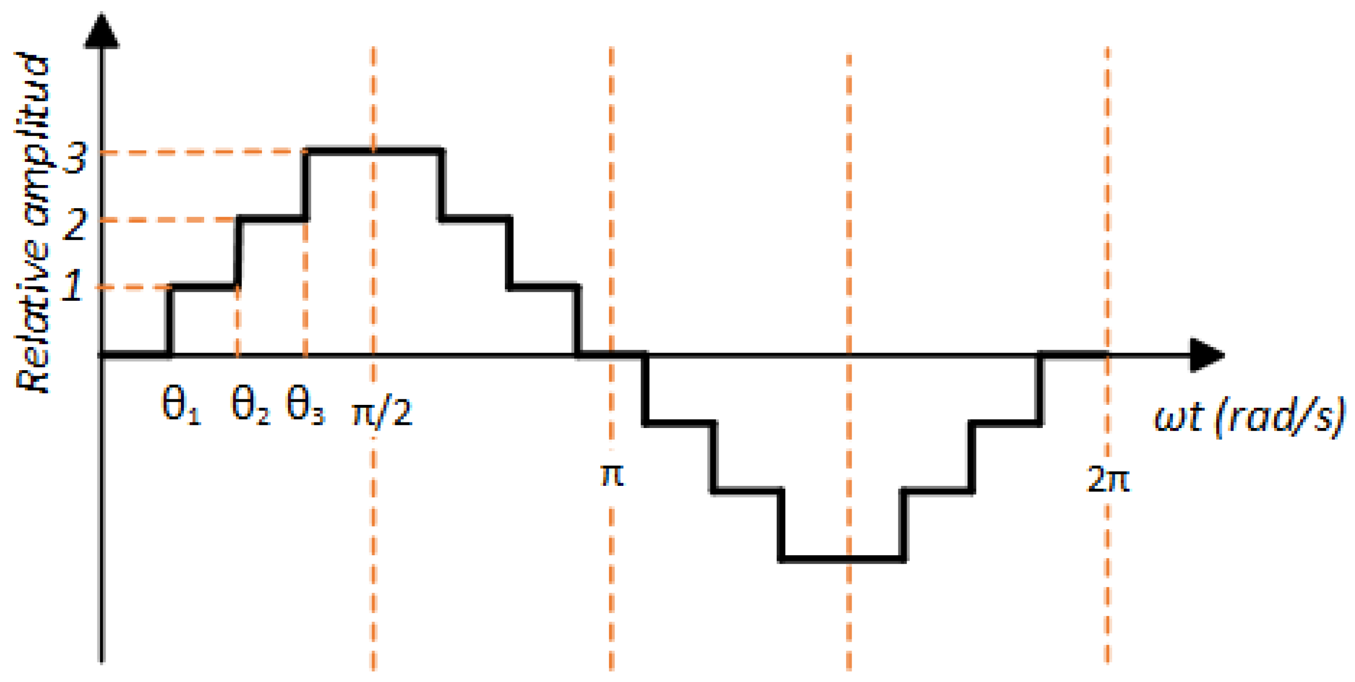
Figure 2 shows the output voltage waveform for a seven-level CHBMLI configuration. Within this context, the angles that should be calculated are θ 1 , θ 2 , and θ 3 .
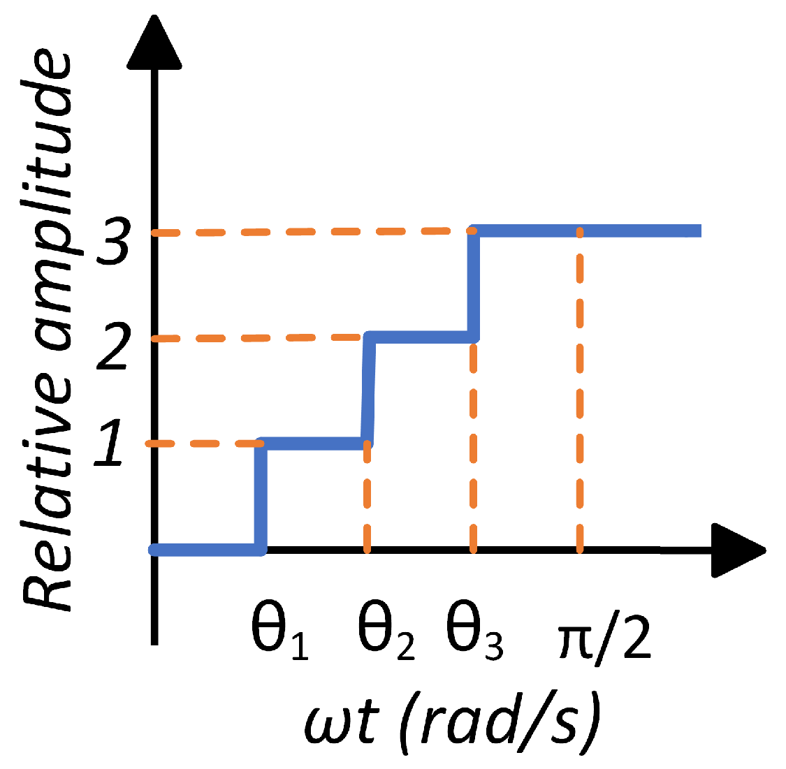
As can be observed in Figure 3, { θ 1 , θ 2 , θ 3 } are the switching angles of the CHBMLI of seven levels during the first quarter of a cycle, which are used to define the switching sequence of the entire cycle. During the first half of the period, the switching angles are, consecutively, θ 1 , θ 2 , θ 3 , π θ 3 , π θ 2 , π θ 1 , and π , while for the second half of the period, the switching angles are π + θ 1 , π + θ 2 , π + θ 3 , 2 π θ 3 , 2 π θ 2 , 2 π θ 1 [12,24].
Then, for this example, the output voltage v o u t ω t is a piece-wise periodic signal with the symmetry of a sine signal and is built from 2 n + 1 integer levels (n positive levels, n negative levels, and zero). In a general way, the output voltage can be defined as a sum of sine and cosine signals expressed by:
v o u t ω t = n = 1 , 3 , 5 , 4 V d c n π k = 1 s c o s n θ k s i n ( n ω t )
where:
n is the odd harmonic order ( 1 , 3 , 5 , 7 , 9 , ) .
s is the number of inverter stages.
k is an integer > 0 .
θ k is the k t h switching angle, which must satisfy:
0 θ 1 < θ 2 < < π 2
where θ 1 can be equal to or greater than zero. The computation of the THD of v o u t ω t can be obtained from (3), and the switching angle calculation determines the output voltage quality [25,26].
T H D ( % ) = 100 V R M S V 1 R M S 1
The RMS of the signal and the RMS of its fundamental component can be obtained from (4) and (5), respectively.
V R M S = n 2 2 π i = 1 n 2 i 1 θ i
V 1 R M S = 4 π 2 c o s θ 1 + + c o s θ n
Minimizing (3) is the optimization objective developed in the following sections.

2.2. Genetic Algorithm

The GA is used for solving both constrained and unconstrained optimization problems based on natural selection principles and genetics [14,27,28,29]. The GA repeatedly modifies a population of individual solutions. At each step, GA performs the following sequential tasks:
  • Population initialization: This is randomly generated and consists of possible solutions to the problem, bounded by the constraints previously defined.
  • Fitness Function: The initial population is evaluated over fitness function to compare one with the other.
  • Selection: This process selects the parents (individuals) from the initial population that makes crossover and permutation to find the next generation.
  • Crossover: Consists of selecting two parents from a population based on fitness function and then changing and improving parent parts to create a new individual.
  • Mutation: This process applies random changes to introduce diversity in the population genes.
  • Reinsertion: The children from the new generation replace some members of the current generation. The new one entirely replaces the current generation.
MATLAB contains a GA solver used in many scientific research communities. However, the GA solver performance maximization requires choosing the appropriate parameters, such as selection function, fitness scaling function, and elite count. Therefore, there are many options, and selecting the proper parameter set is challenging, requiring a systematic approach. For the sake of brevity, the description of the GA solver parameters is not discussed in this paper; however, a detailed description can be found in MATLAB quick reference for this solver.
This paper takes the Taguchi experimental design proposal exposed in [28] to acquire the appropriate GA-solver parameters, leading to the switching angles of five, seven, and nine multilevel cascaded inverters. This proposal prevents the trial-and-error method in the GA solver, and a better THD is obtained compared to other papers in the literature under the same characteristics, such as the same objective function and the same harmonic spectrum.

2.3. Taguchi Method

Genichi Taguchi developed the Taguchi method; the objective was to improve the quality of the produced goods, but it was later implemented in other applications, like marketing, engineering, and biotechnology, among others [18,19,20,21,23,30].
Taguchi created standard orthogonal arrays (OA) to facilitate the efficient evaluation of multiple parameters and their impact on the variability of specific product or process characteristics. Utilizing these OAs makes it possible to simultaneously and independently assess two or more parameters while conducting the minimum required number of tests [21,23,31]. The OAs are designed with the orthogonality property. These designs depend on the number of factors to study in a particular case. For example, the OA L 8 has eight experimental runs, and up to seven factors of two levels each can be studied.
The results are analyzed once the experiments are conducted to determine the optimal parameter configuration within the experiment design. In analyzing the results, a loss function is defined to calculate the deviations between the experimental value and the desired one. This loss function is transferred to a statistical measure of performance called signal-to-noise (S/N) ratio, η . Dr. Taguchi introduced the S/N ratio as a metric for selecting optimal control levels that effectively manage noise. This ratio considers both the average performance and the variability. Essentially, the S/N ratio, in its basic form, represents the relationship between the average value (signal) and the standard deviation (noise). The specific formulation of the S/N equation varies based on the quality characteristic criteria targeted for optimization [32].
There are three S/N ratios available, depending on the type of characteristic: the lower, the better (LB); the higher, the better (HB); and the nominal, the better (NB) [30,31]. Each S/N ratio is calculated as shown.
Nominal is the best:
S N N B = 10 l o g y ¯ s y 2
Larger is the better (maximize):
S N L B = 10 l o g 1 n i = 1 n 1 y i 2
Smaller is the better (minimize):
S N S B = 10 l o g 1 n i = 1 n y i 2
where y ¯ is the average of the observed data, s y 2 is the variance of y, n is the number of observations, and y is the observed data. Regardless of the chosen category, the more excellent S/N ratio corresponds to the better performance characteristics, so the optimal level of the parameters is that with the highest S/N ratio η . In this paper, to obtain a low THD in the GA solver of MATLAB for the five and seven multilevel inverters, the used parameters were taken from [28] and are listed in Table 1.
It is important to note that the parameter named “migration direction” has two levels, while the rest of the variables have four; this leads to choosing the Taguchi orthogonal design L 32 ( 2 1 4 8 ) . This design was implemented in the software Minitab, which yields the experiment layout shown in Table 2. Each experiment must be repeated several times to increase the experiment response consistency. In this case, each experiment is repeated up to four times, while the chosen computing time for each experiment was thirty seconds.
The experiments shown in Table 2 were conducted by considering the objective function of (3), where the objective was to obtain the appropriate switching angles for the five- and seven-level inverters, and therefore, a low THD value.

2.4. Taguchi Results Analysis

The experiments in Table 2 were carried out in the MATLAB solver for five- and seven-level CHBMLI. The analysis of the results of the experiments was carried out with the Minitab software. The Minitab software made the Taguchi analysis, and the S/N plots were obtained.

2.4.1. Five-Level Results

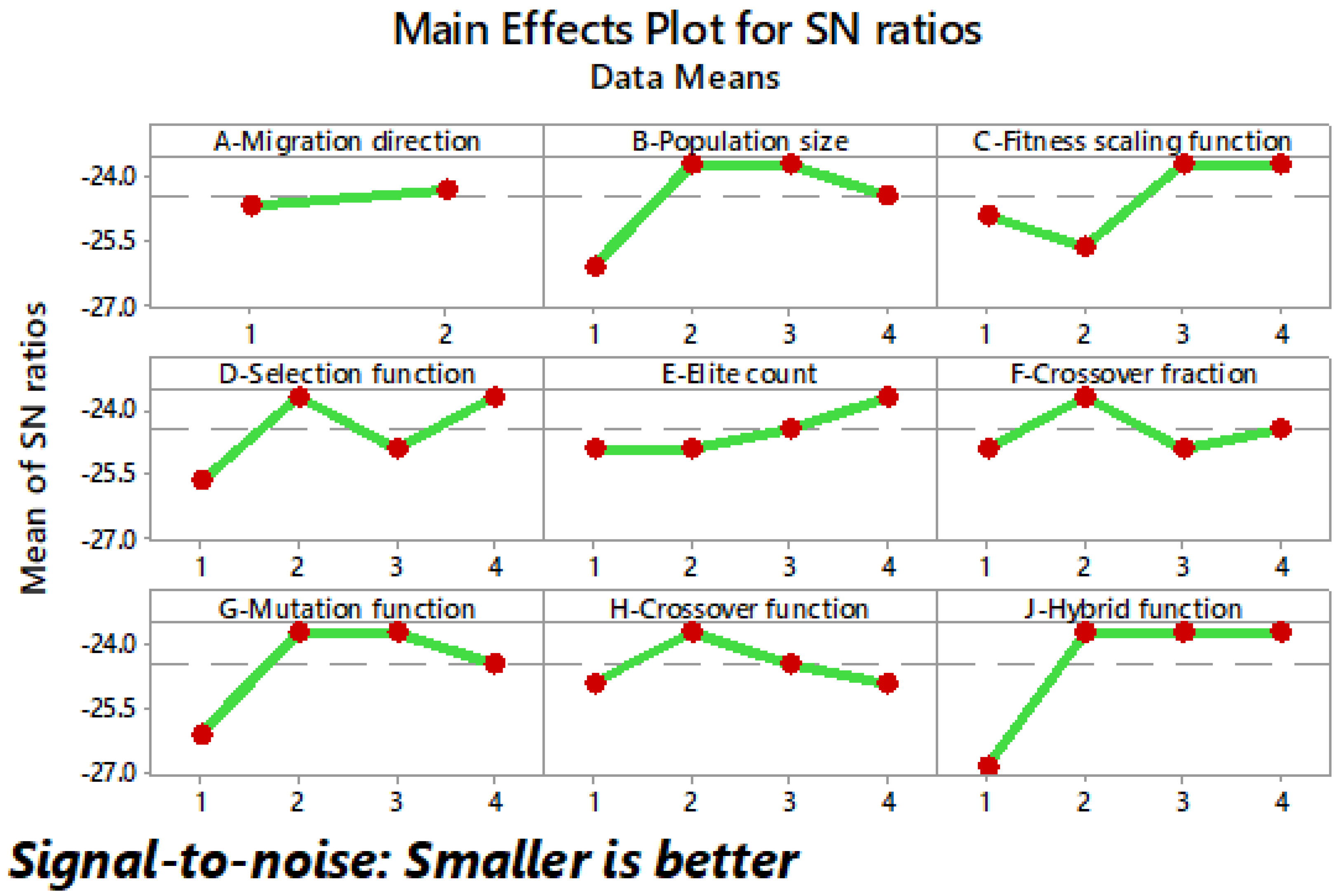
Figure 4 shows the S/N plot of the levels considered during the Taguchi analysis. In the graph presented, each level is analyzed to understand its influence on the system performance. By applying the Taguchi methodology, it is possible to identify the levels that contribute most significantly to the desired performance. These results were based on the appropriate selection of the smaller-is-better function [33].
These graphs visualize which effects may be more significant: the further a point is from the horizontal dotted line, the more critical the corresponding effect is, and the more inclined the line is, the more sensitive it is. The sensitivity of a factor is the ability of that factor to influence the final results of the system through adjustments in its levels. Those that are insignificant tend to form a straight line, while the less essential points are far from the dotted line [34].
In this case, factor A reveals an almost-horizontal trend, indicating that the modification of this parameter does not have a relevant influence on the THD value. On the contrary, factors B, G, and J are presented with considerable inclinations, which indicates the possibility of being more sensitive than the rest of the other factors.
From Figure 4, the combination that leads to a low THD for the objective function shown in (3) can be identified. The points above this line are observed based on the horizontal dotted line. Among these points, the optimal levels are selected for each factor (understood as levels as the specific values assigned to each factor). The optimal points are those that are furthest above the dotted line. Table 3 shows the configuration for each factor.
The parameters of Table 3 were implemented in the MATLAB GA toolbox, obtaining the following angles: θ 1 = 13.406 and θ 2 = 41.915 . With these angles, it was obtained a theoretical THD of 15.299 % .

2.4.2. Seven-Level Results

Just like the five-level results, in Figure 5, the main effects graphs for the inverter of seven levels are observed when examining the S/N graphical representations; in this case, the G factor is distinguished, which reveals an almost-horizontal trend, thus hinting at its lack of sensitivity or influence when obtaining the THD value. On the contrary, factors C, D, and J are presented with considerable inclinations, pointing to the possibility of being more sensitive than the rest of the other factors.
Table 4 shows the combination that leads to a low THD. This combination is obtained by selecting the optimal levels from Figure 5. As in the five-level results, this selection is made by choosing the points furthest above the dotted line.
By implementing the parameters of Table 4 into the MATLAB GA toolbox, the following angles were obtained: θ 1 = 8.692 , θ 2 = 27.896 , and θ 3 = 49.817 . These angles lead to a theoretical THD of 10.432 % . The Table 5 shows the obtained results for both cases. These angles were implemented in a laboratory prototype, and the resulting THDs for both cases are showed in the next section.

3. Results

An H-bridge inverter was built to implement the obtained angles of Table 5. The inverter used STGW20NC60VD IGBTs as switching semiconductors and was replicated up to three times to obtain the five- and seven-level CHBMLI. The peak voltage to each cascaded H-bridge inverter is 180 V; this means that for a five-level cascaded H-bridge inverter, two voltage sources of 90 V each were used as an input, while three voltages of 60 V were used for a seven-level cascaded H-bridge inverter.
Figure 6 shows the five-level inverter setup with a resistive load. A frequency of 60 Hz with a resistive and an RL load was used in both cases. The sequence of the switching angles obtained from the presented methods was programmed in a PIC16F877A, which provides the gate signals applied to the inverter bridges through ACPL3130 drivers. These switching angles are those shown in Table 5.
The set of instruments used for the measurements is listed in Table 6. The form of the voltage output was verified with the oscilloscope, while the output voltage THD was verified with the power quality analyzer.

3.1. Five-Level Implementation Results

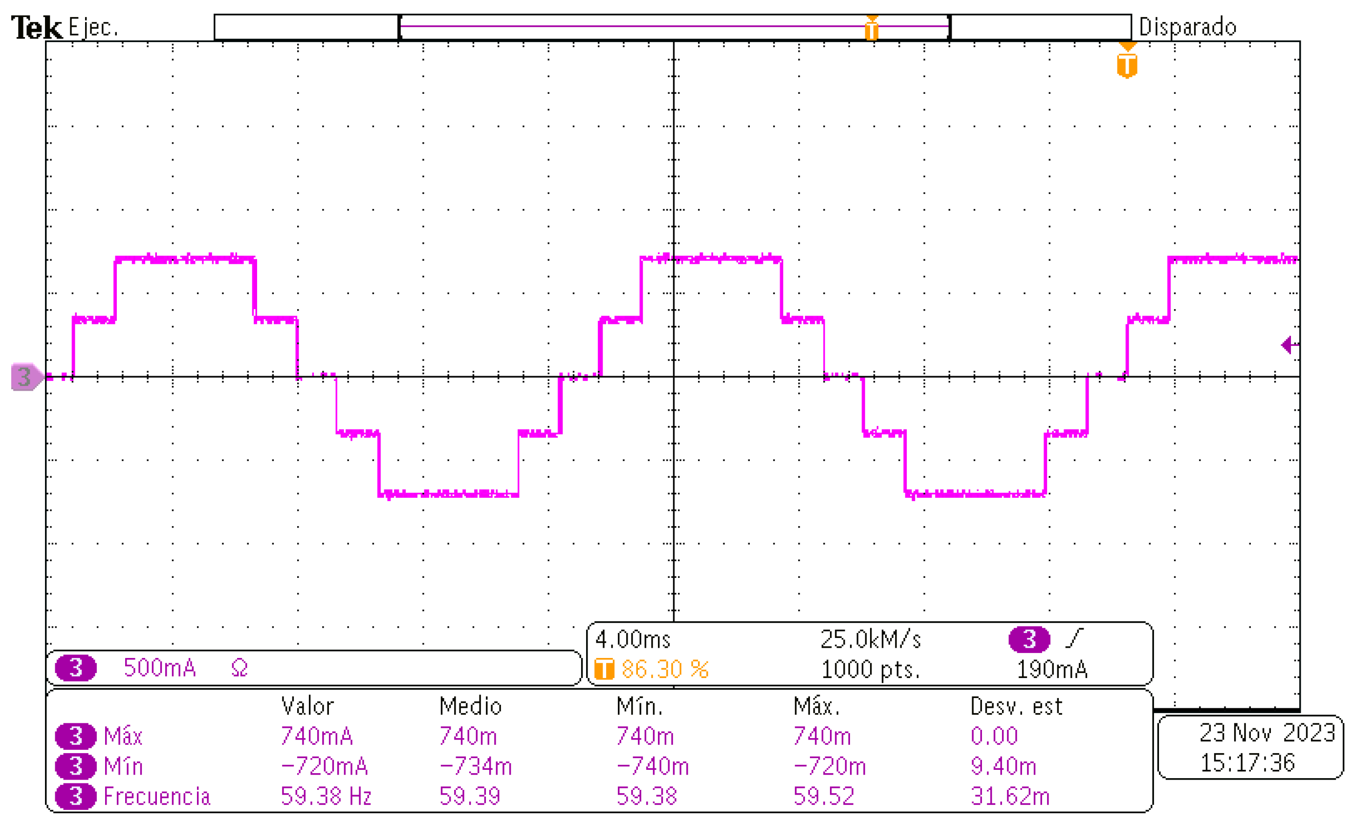
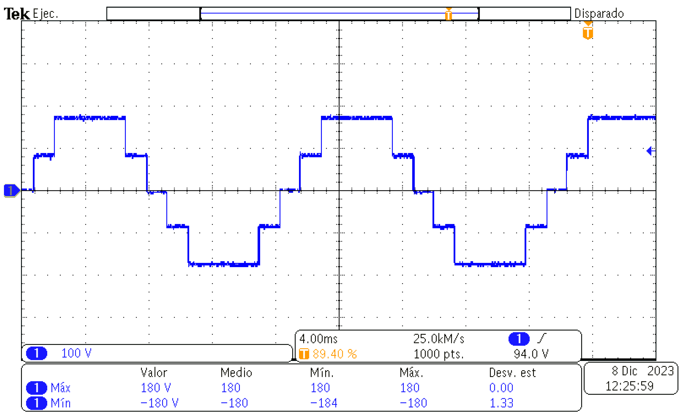
Figure 7 illustrates the voltage output waveform for the five levels of CHBMLI with a load of 250 ω . The peak voltage of the signal stands at 180 V, as initially intended, and the frequency closely approximates 60 Hz. This figure was captured using the oscilloscope, and it is evident that the five output levels are distinctly defined. It is essential not to forget that this waveform was generated with the previous angles of θ 1 = 13.406 and θ 2 = 41.915 . Figure 8 shows the current output waveform: this signal has the same form as Figure 7 because the load of the five-levels CHBMLI is resistive.
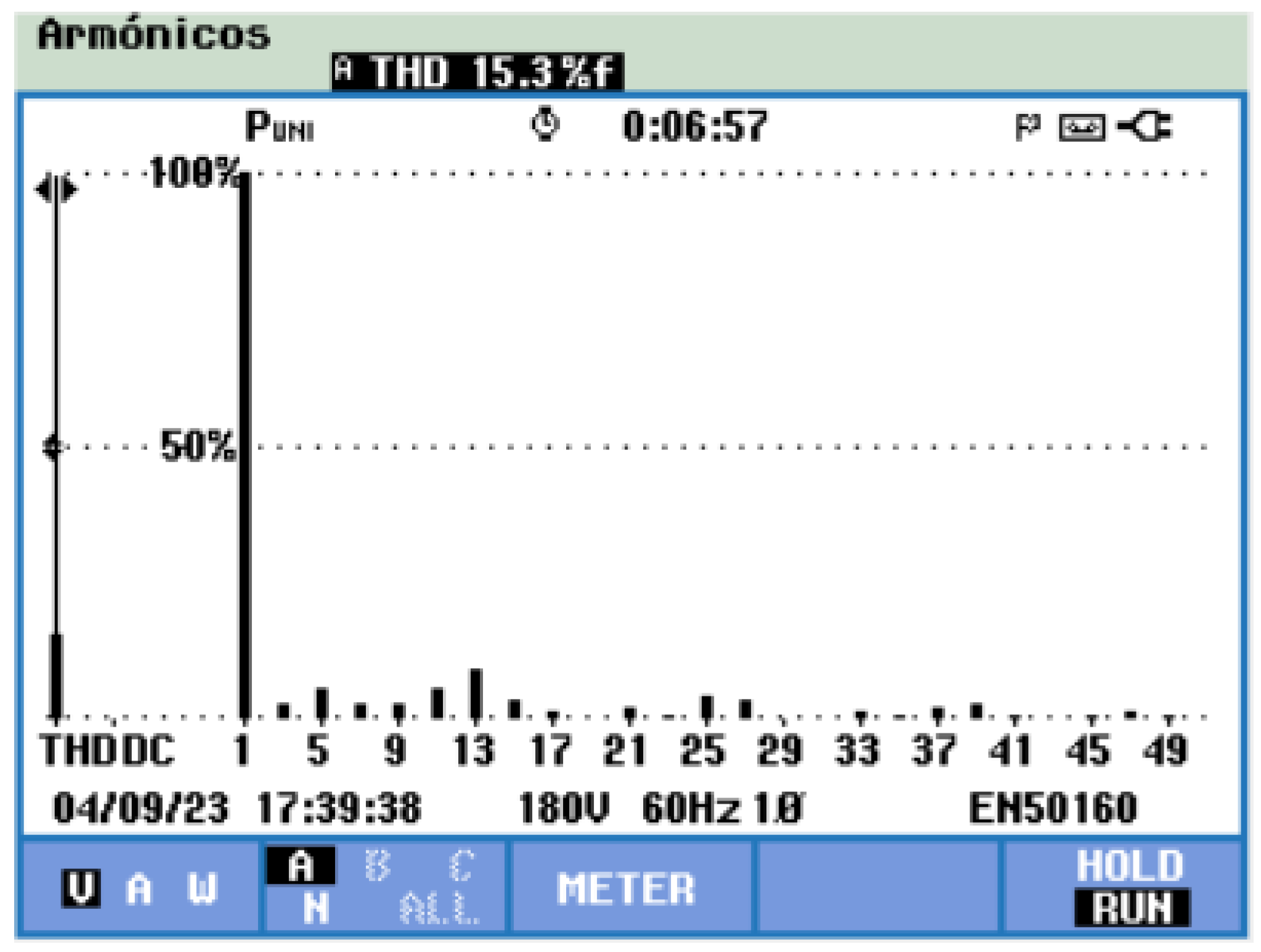
Figure 9 displays the fast Fourier transform (FFT) of Figure 7, which was acquired using the power quality analyzer, encompassing harmonics up to the 49th order. According to this figure, the THD value is 15.3 % , almost identical to the theoretical value of 15.299 % reported in Table 5.
Then, the five-level CHBMLI was tested with an RL load. The resistive load remained with a value of 250 Ω , while the inductive consisted of a brushless AC motor, as shown in Figure 10. Table 7 shows its main aspects.
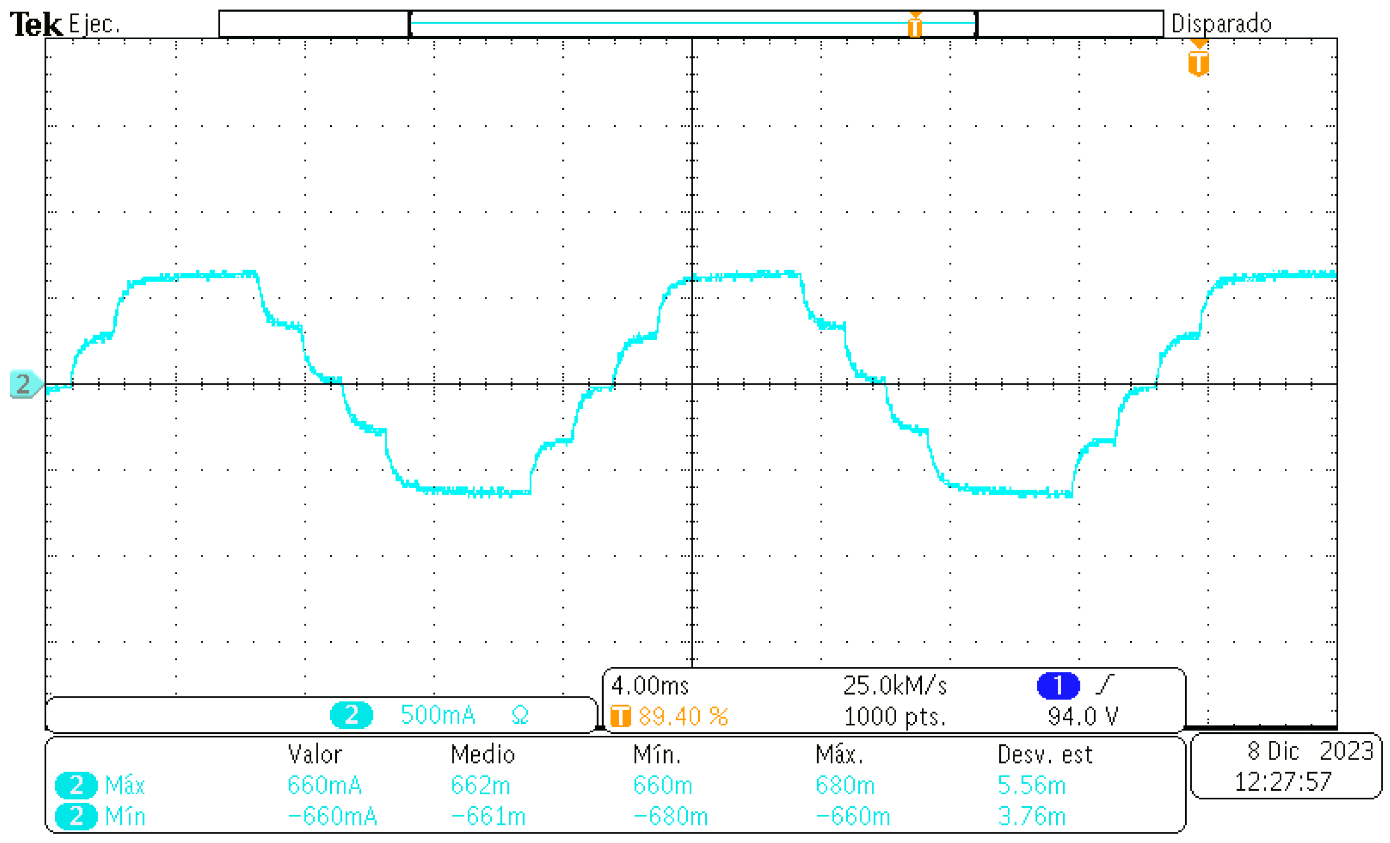
The output voltage with the RL load is shown in Figure 11, while the output current is shown in Figure 12. Due to the presence of an inductive component in the load, the output current waveform deviates from matching the output voltage waveform.
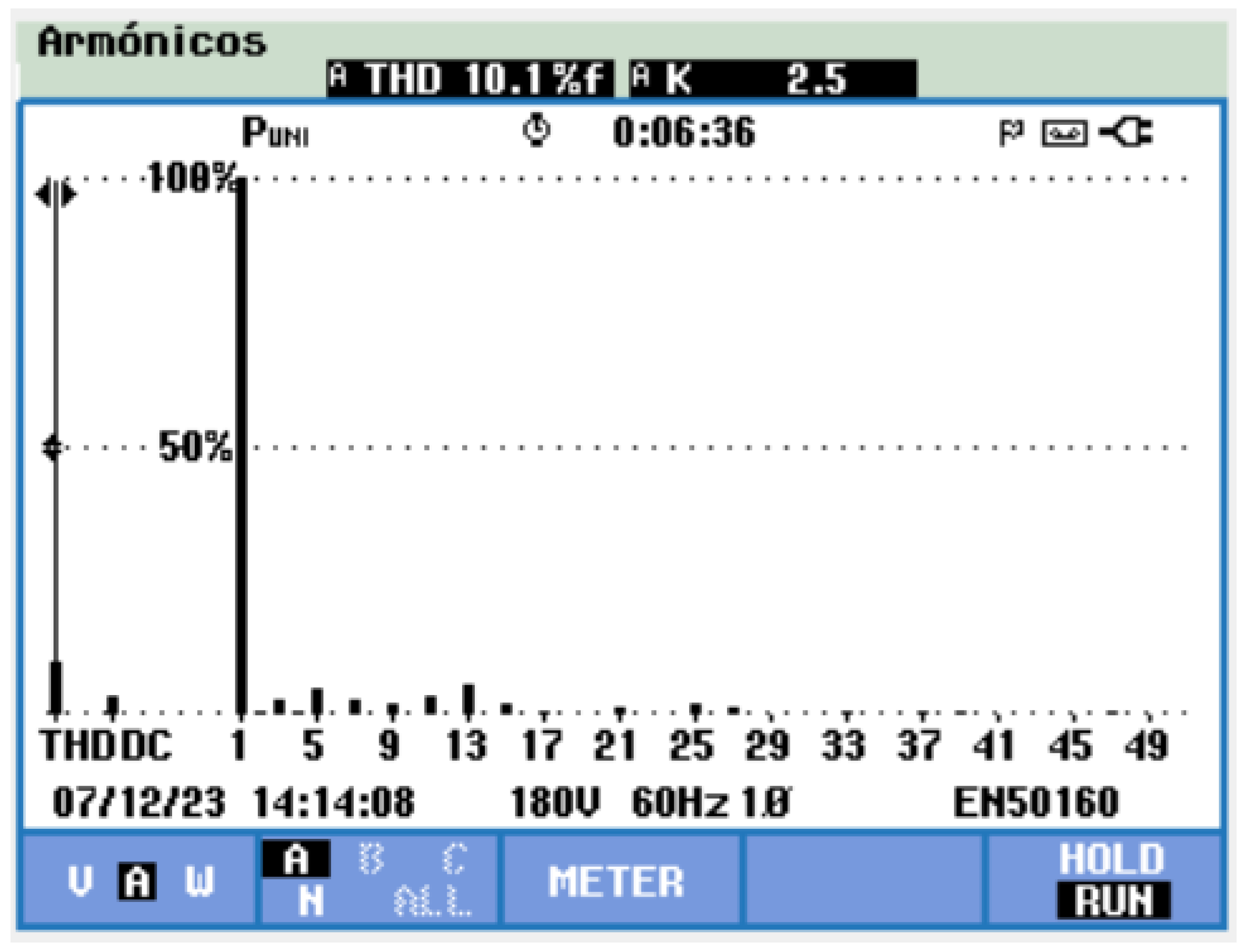
The THD voltage value is the same with the purely resistive load and the inductive load since the waveform remains practically unchanged. However, the THD of the current decreases to 10.1 % , lower than the THD voltage level, as shown in Figure 13.

3.2. Seven-Level Implementation Results

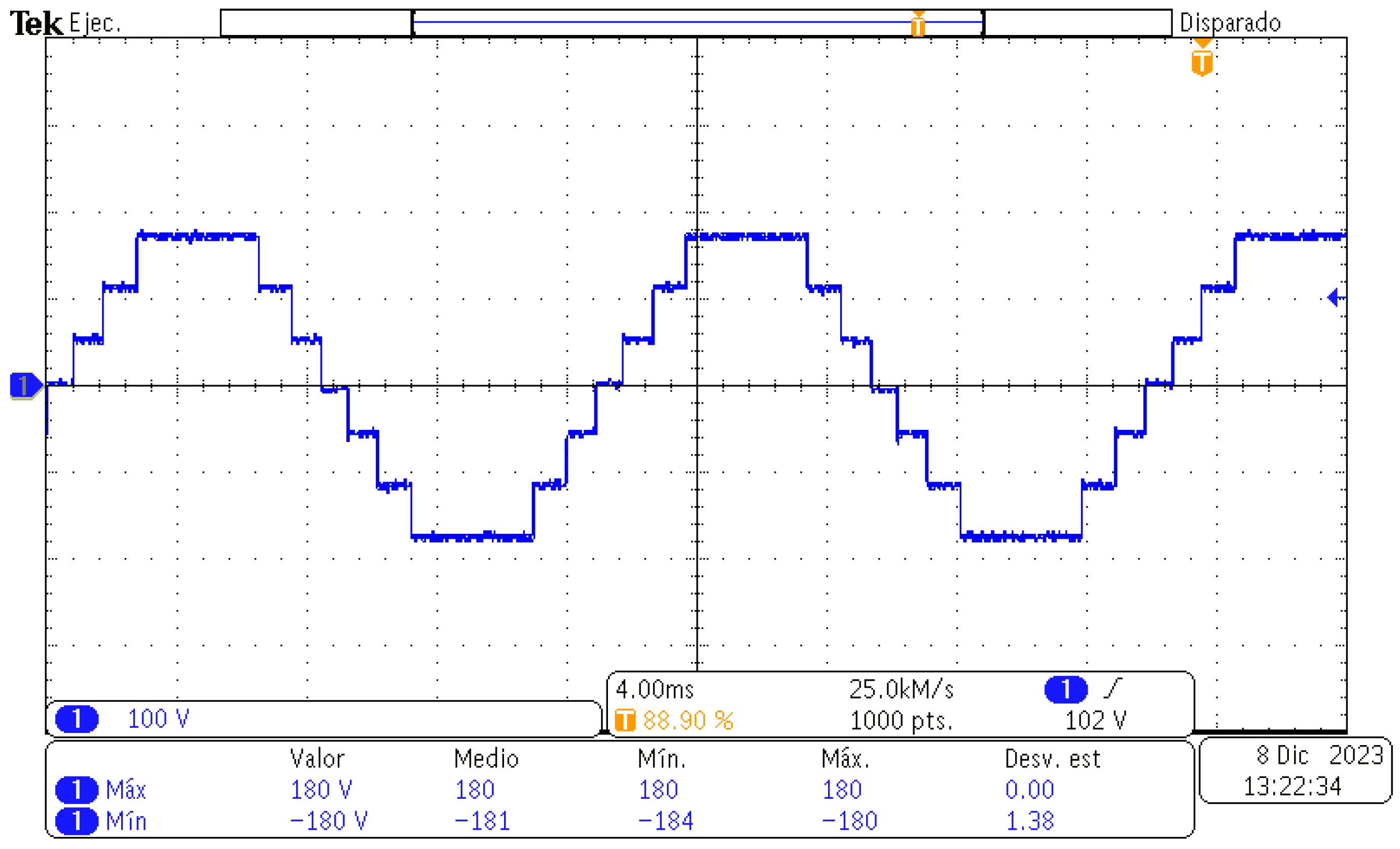
Regarding the results of the implementation of the seven-level CHBMLI, Figure 14 shows the output voltage waveform with the resistive load of 250 Ω , while Figure 15 shows the corresponding output current waveform. Like the previous results, the well-defined levels of the voltage waveform obtained with the oscilloscope can also be observed: in this case, there are seven levels, and the frequency is near 60 Hz. This waveform was obtained through the following previously obtained angles: θ 1 = 8.692 , θ 2 = 27.896 , and θ 3 = 49.817 .
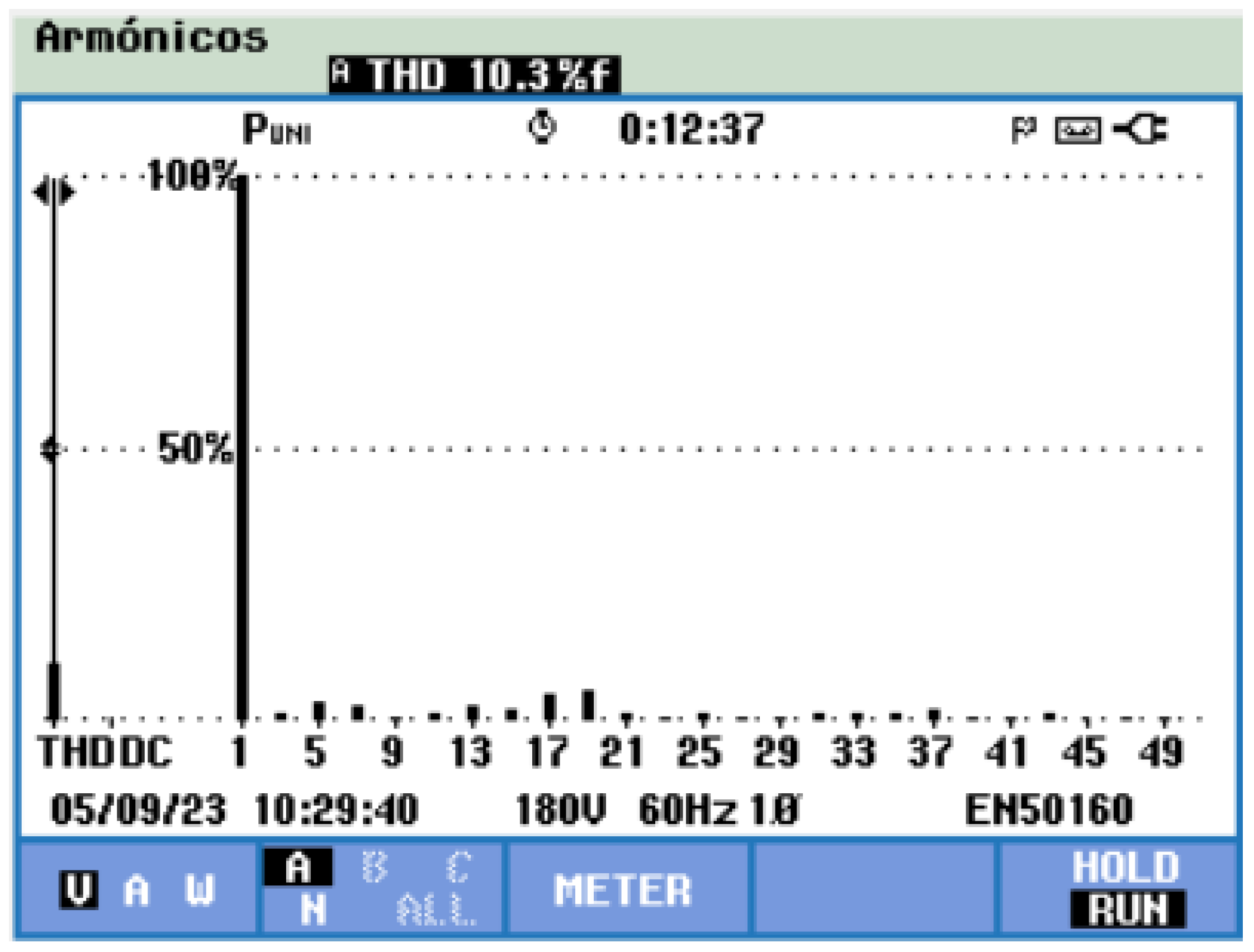
Figure 16 shows the FFT of Figure 14 with its corresponding THD value. In this case, the obtained THD value in the prototype was 10.3 % , while the theoretical THD shown in Table 5 is 10.432 % .
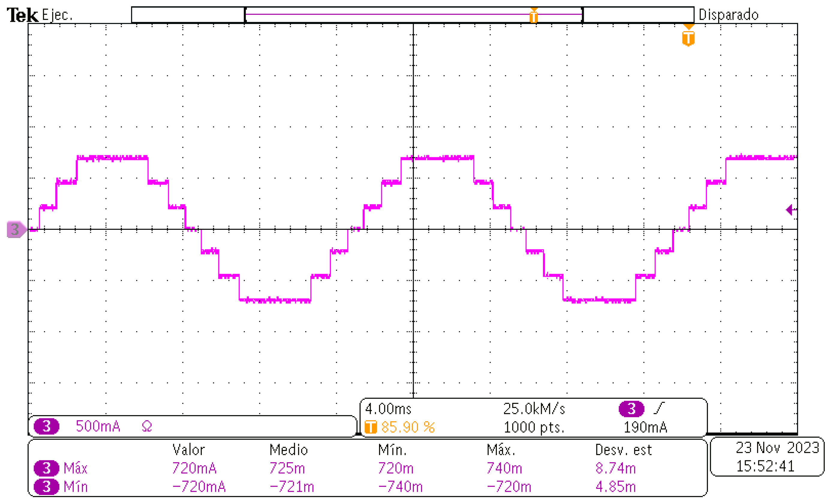
In the same way that the tests were performed with the five-level CHBMLI, the seven-level inverter was tested with the RL load described before. Figure 17 shows the voltage output of the seven-level CHBMLI with RL load, while Figure 18 shows its current output.
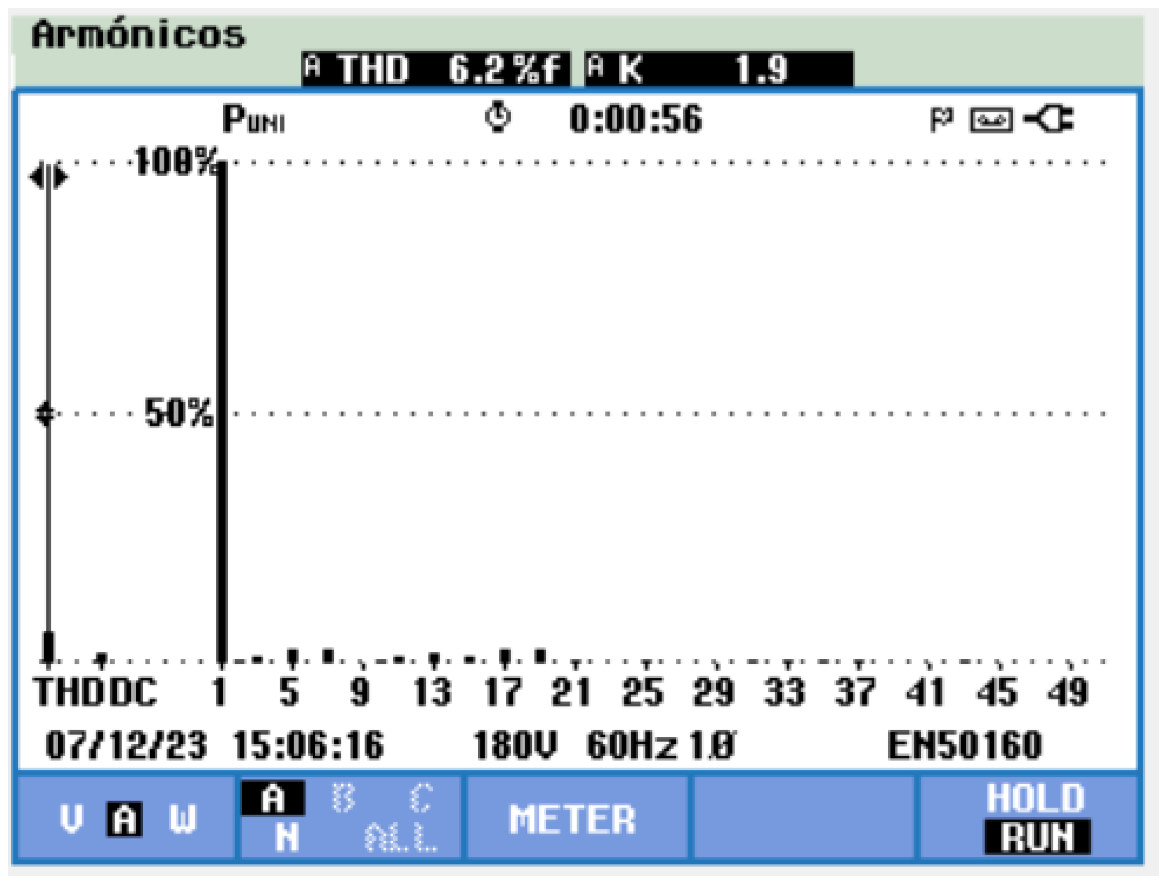
The voltage output maintains its shape, and the THD value of the current decreased at 6.2 % , as can be seen in Figure 19.
Table 8 shows the theoretical and experimental results for the THD voltage value for the five- and seven-level CHBMLI. The results show the proximity between the theoretical and the experimental THD. The experimental results for the seven-level CHBMLI gave a lower THD value for the seven-level CHBMLI.

4. Discussion

As previously stated, GA parameters are commonly chosen by trial and error, which may not guarantee the lowest THD value. Due to the above, and to verify the effectiveness of implementing the Taguchi method, the value of the THD obtained in this paper was compared to some other papers presented in the literature that use the same objective function (shown in (3)) and the same algorithm (GA). Table 9 shows the THD comparison of the five-level CHBMLI, while Table 10 shows the THD comparison of the seven-level CHBMLI.
In ref. [14], the authors show the obtained THD value by simulation for the five- and seven-level CHBMLI. A table with the used parameters for the GA is given; however, there is no explanation of how these parameters were chosen.
The authors of [35] use the exact MATLAB GA solver that is used in this paper; however, the authors do not state how the GA parameters were chosen. This THD value reported in this paper was lower in both cases, and the results were obtained experimentally.
It is essential to mention that for the comparison, only articles where the harmonic spectrum reached the 49th harmonic were considered. Some articles were found where the same objective function was considered, but the range of the harmonic spectrum differed from that in this paper. For example, in ref. [15], it is considered up to the 40th harmonic, while in ref. [36] it is considered up to the 100th harmonic. Due to the above, these articles were not considered since it would be impossible to compare this paper correctly.

5. Conclusions

This paper highlights the determination of optimal switching angles for both five- and seven-level CHBMLI to minimize the THD in the output voltage waveform. The switching angles were calculated using the MATLAB GA solver. Instead of relying on the traditional trial-and-error or user experience approach to configuring the solver parameters, this study employed the Taguchi method, providing a more systematic and efficient parameter tuning.
These determined switching angles were subsequently applied to a CHBMLI laboratory prototype, and THD measurements were conducted for the five- and seven-level configurations. A comparison was made between the experimental THD values and their theoretical counterparts, revealing a maximum deviation of only 0.132 % .
In addition, the study compares these optimized switching angles and experimental THD values with data from the existing literature that utilized the same objective function and harmonic spectrum. Remarkably, the results demonstrate that the Taguchi method leads to lower THD values in five- and seven-level CHBMLIs than previously reported results. This observation highlights the potential of the Taguchi method for application in other optimization techniques, such as particle swarm optimization (PSO) and the artificial bee colony (ABC) algorithm, among others.

Author Contributions

Conceptualization, A.R.L. and O.L.-S.; methodology, J.M.S. and C.S.; software, C.S.; validation, S.E.D.L.-A. and J.A.-A.; formal analysis, A.R.L. and O.L.-S.; investigation, A.R.L. and C.S.; resources, S.E.D.L.-A. and J.A.-A.; writing—original draft preparation, A.R.L.; writing—review and editing, J.M.S.; visualization, S.E.D.L.-A.; supervision, J.A.-A.; project administration, A.R.L.; funding acquisition, A.R.L. All authors have read and agreed to the published version of the manuscript.

Funding

This research was funded by the government of the Guanajuato state through “IDEA GTO” under grant IDEAGTO/CONV/071/2023.

Data Availability Statement

The data presented in this study are available on request from the corresponding author.

Conflicts of Interest

The authors declare no conflict of interest.

References

  1. Rodríguez, J.; Lai, J.S.; Fang, Z. Multilevel Inverters: A Survey of Topologies, Controls, and Applications. IEEE Trans. Ind. Electron. 2002, 49, 724–738. [Google Scholar] [CrossRef]
  2. Franquelo, L.G.; Rodriguez, J.; Leon, J.I.; Kouro, S.; Portillo, R.; Prats, M.A. The age of multilevel converters arrives. IEEE Ind. Electron. Mag. 2008, 2, 28–39. [Google Scholar] [CrossRef]
  3. Garcia-Santiago, F.A.; Rosas-Caro, J.C.; Valdez-Resendiz, J.E.; Mayo-Maldonado, J.C.; Valderrabano-Gonzalez, A.; Robles-Campos, H.R. Single-Phase Five-Level Multilevel Inverter Based on a Transistors Six-Pack Module. Energies 2022, 15, 9321. [Google Scholar] [CrossRef]
  4. Malinowski, M.; Gopakumar, K.; Rodriguez, J.; Perez, M.A. A survey on cascaded multilevel inverters. IEEE Trans. Ind. Electron. 2010, 57, 2197–2206. [Google Scholar] [CrossRef]
  5. Colak, I.; Kabalci, E.; Bayindir, R. Review of multilevel voltage source inverter topologies and control schemes. Energy Convers. Manag. 2011, 52, 1114–1128. [Google Scholar] [CrossRef]
  6. Koshti, A.K.; Rao, M. A Brief review on multilevel inverter topologies. In Proceedings of the 2017 International Conference on Data Management, Analysis and Innovation (ICDMAI), Pune, India, 24–26 February 2017; pp. 187–193. [Google Scholar]
  7. Balal, A.; Dinkhah, S.; Shahabi, F.; Herrera, M.; Chuang, Y.L. A Review on Multilevel Inverter Topologies. Emerg. Sci. J. 2022, 6, 185–200. [Google Scholar] [CrossRef]
  8. Ebrahimi, J.; Babaei, E.; Gharehpetian, G. A New Topology of Cascaded Multilevel Converters with Reduced Number of Components for High-Voltage Applications. IEEE Trans. Power Electron. 2011, 26, 3109–3118. [Google Scholar] [CrossRef]
  9. Bughneda, A.; Salem, M.; Richelli, A.; Ishak, D.; Alatai, S. Review of multilevel inverters for PV energy system applications. Energies 2021, 14, 1585. [Google Scholar] [CrossRef]
  10. Edpuganti, A.; Rathore, A.K. A Survey of Low Switching Frequency Modulation Techniques for Medium-Voltage Multilevel Converters. In Proceedings of the 2014 IEEE Industry Application Society Annual Meeting, Vancouver, BC, Canada, 5–9 October 2014; pp. 1–8. [Google Scholar] [CrossRef]
  11. Ahmed, A.; Sundar Manoharan, M.; Park, J.H. An Efficient Single-Sourced Asymmetrical Cascaded Multilevel Inverter with Reduced Leakage Current Suitable for Single-Stage PV Systems. IEEE Trans. Energy Convers. 2019, 34, 211–220. [Google Scholar] [CrossRef]
  12. José, R.; Franquelo, L.G.; Samir, K.; León, J.I.; Portillo, R.C.; Prats, M.Á.M.; Pérez, M.A. Multilevel converters: An enabling technology for high-power applications. Proc. IEEE 2009, 97, 1786–1817. [Google Scholar] [CrossRef]
  13. Choupan, R.; Golshannavaz, S.; Nazarpour, D.; Barmala, M. A new structure for multilevel inverters with fault-tolerant capability against open circuit faults. Electr. Power Syst. Res. 2019, 168, 105–116. [Google Scholar] [CrossRef]
  14. Reyes, M.M.; Alquicira, J.A.; De Leon Aldaco, S.; Amores Campos, E.M.; Severiano, Y.R. Calculation of optimal switching angles for a multilevel inverter using NR and GA—A comparison. In Proceedings of the International Power Electronics Congress—CIEP, Cholula, Mexico, 24–26 October 2018; pp. 22–27. [Google Scholar] [CrossRef]
  15. Araque, G.J.A.; Díaz, R.J.L.; Gualdrón, G.O.E. The optimization of a single phase multilevel inverter using genetic algorithms. Rev. Colomb. Tecnol. Avanzada 2013, 1, 60–66. [Google Scholar]
  16. Ten, V.; Matkarimov, B.; Isembergenov, N. Using Genetic Algorithm and Single-phase Multilevel DC/AC Converter for the Fuel Cells Supporting System. In Proceedings of the 16th International Power Electronics and Motion Control Conference and Exposition, Antalya, Turkey, 21–24 September 2014; pp. 600–603. [Google Scholar]
  17. PrasadPanda, K.; Prasad Sahu, B.; Samal, D.; Gopal, Y. Switching Angle Estimation using GA Toolbox for Simulation of Cascaded Multilevel Inverter. Int. J. Comput. Appl. 2013, 73, 21–26. [Google Scholar] [CrossRef]
  18. Guharaja, S.; Noorul Haq, A.; Karuppannan, K.M. Optimization of green sand casting process parameters by using Taguchi’s method. Int. J. Adv. Manuf. Technol. 2006, 30, 1040–1048. [Google Scholar] [CrossRef]
  19. Syrcos, G.P. Die casting process optimization using Taguchi methods. J. Mater. Process. Technol. 2003, 135, 68–74. [Google Scholar] [CrossRef]
  20. Wei, S.; Ye, L.; Shaokun, Z.; Qibiao, S. Optimal Design of PCB Layout Based on Thermal Analysis Using Taguchi Method. In Proceedings of the 2021 3rd Asia Energy and Electrical Engineering Symposium, AEEES, Chengdu, China, 26–29 March 2021; pp. 198–202. [Google Scholar] [CrossRef]
  21. Byun, H.S.; Lee, S.H. Design of a piston forging process using a hybrid Taguchi method and multiple criteria decision-making. J. Mech. Sci. Technol. 2017, 31, 1869–1876. [Google Scholar] [CrossRef]
  22. Kirby, E.D.; Zhang, Z.; Chen, J.C.; Chen, J. Optimizing surface finish in a turning operation using the Taguchi parameter design method. Int. J. Adv. Manuf. Technol. 2006, 30, 1021–1029. [Google Scholar] [CrossRef]
  23. Semioshkina, N.; Voigt, G. An overview on Taguchi Method. J. Radiat. Res. 2006, 47 (Suppl. A), A95–A100. [Google Scholar] [CrossRef]
  24. Babaei, E.; Kangarlu, M.F.; Sabahi, M.; Pahlavani, M.R.A. Cascaded multilevel inverter using sub-multilevel cells. Electr. Power Syst. Res. 2013, 96, 101–110. [Google Scholar] [CrossRef]
  25. Sánchez Vargas, O.; De León Aldaco, S.E.; Aguayo Alquicira, J.; Vela Valdés, L.G.; Mina Antonio, J.D. Differential Evolution Applied to a Multilevel Inverter—A Case Study. Appl. Sci. 2022, 12, 9910. [Google Scholar] [CrossRef]
  26. Gómez Díaz, K.Y.; De León Aldaco, S.E.; Aguayo Alquicira, J.; Ponce-Silva, M.; Olivares Peregrino, V.H. Teaching–Learning-Based Optimization Algorithm Applied in Electronic Engineering: A Survey. Electronics 2022, 11, 3451. [Google Scholar] [CrossRef]
  27. Haldurai, L.; Madhubala, T.; Rajalakshmi, R. A Study on Genetic Algorithm and its Applications. Int. J. Comput. Sci. Eng. 2016, 4, 139–143. [Google Scholar]
  28. Son Duy, L.; Abhary, K.; Romeo, M. Maximising Performance of Genetic Algorithm Solver in Matlab. Eng. Lett. 2016, 24. [Google Scholar]
  29. Elmas, C.; Yigit, T. Genetic algorithm based on-line tuning of a PI controller for a switched reluctance motor drive. Electr. Power Components Syst. 2007, 35, 675–691. [Google Scholar] [CrossRef]
  30. Gaing, Z.L.; Wang, Q.Q.; Chiang, J.A. Optimization of in-wheel PM motor by fuzzy-based Taguchi method. In Proceedings of the 2010 International Power Electronics Conference—ECCE Asia—IPEC 2010, Sapporo, Japan, 21–24 June 2010; Volume 821, pp. 1312–1316. [Google Scholar] [CrossRef]
  31. Hasçalik, A.; Çaydaş, U. Optimization of turning parameters for surface roughness and tool life based on the Taguchi method. Int. J. Adv. Manuf. Technol. 2008, 38, 896–903. [Google Scholar] [CrossRef]
  32. Madu, I.E.; Madu, C.N. Design optimization using signal-to-noise ratio. Simul. Pract. Theory 1999, 7, 349–372. [Google Scholar] [CrossRef]
  33. Cruz, E.A.; Medina, P.D.; Silva, C.A. A critical review of the signal to noise methodology used in the Taguchi. Sci. Tech. 2012, XVII, 52–56. [Google Scholar]
  34. Roy, R.K. A Primer on the Taguchi Method, 2nd ed.; Society of Manufacturing Engineers: Southfield, MI, USA, 2010. [Google Scholar]
  35. Marín-Reyes, M.; Aguayo-Alquicira, J.; De León-Aldaco, S.E. Calculation of Optimal Switching Angles for a Multilevel Inverter Using NR, PSO, and GA- a Comparison. Eur. J. Electr. Eng. 2020, 22, 349–355. [Google Scholar] [CrossRef]
  36. Yousefpoor, N.; Fathi, S.H.; Farokhnia, N.; Abyaneh, H.A. THD Minimization Applied Directly on the Line-to-Line Voltage of Multilevel Inverters. IEEE Trans. Ind. Electron. 2012, 59, 373–380. [Google Scholar] [CrossRef]
Figure 1. General topology of the CHBMLI.
Machines 12 00007 g001
Figure 2. Seven-level CHBMLI voltage, each long vertical line represents a quarter of the cycle.
Machines 12 00007 g002
Figure 3. A quarter-cycle of a seven-level signal voltage, each line aligns the relative magnitude with its respective θ .
Machines 12 00007 g003
Figure 4. Main effects plots of S/N ratios for the 5-level inverter.
Machines 12 00007 g004
Figure 5. Main effects plots of S/N ratios for the 7-level inverter.
Machines 12 00007 g005
Figure 6. Laboratory setup.
Machines 12 00007 g006
Figure 7. Output voltage of the five-level CHBMLI with resistive load.
Machines 12 00007 g007
Figure 8. Output current of the five-level CHBMLI with resistive load.
Machines 12 00007 g008
Figure 9. Harmonic spectrum and THD value of the five-level CHBMLI.
Machines 12 00007 g009
Figure 10. Brushless AC motor.
Machines 12 00007 g010
Figure 11. Output voltage of the five-level CHBMLI with RL load.
Machines 12 00007 g011
Figure 12. Output current of the five-level CHBMLI with RL load.
Machines 12 00007 g012
Figure 13. Harmonic spectrum and THD value of the five-level CHBMLI with RL load.
Machines 12 00007 g013
Figure 14. Output voltage of the seven-level CHBMLI.
Machines 12 00007 g014
Figure 15. Output current of the seven-level CHBMLI.
Machines 12 00007 g015
Figure 16. Harmonic spectrum and THD value of the seven-level CHBMLI.
Machines 12 00007 g016
Figure 17. Output voltage of the seven-level CHBMLI with RL load.
Machines 12 00007 g017
Figure 18. Output current of the seven-level CHBMLI with RL load.
Machines 12 00007 g018
Figure 19. Harmonic spectrum and THD value of the seven-levels CHBMLI with RL load.
Machines 12 00007 g019
Table 1. Solver parameters and experimental levels.
No.ParameterCodeLevel 1Level 2Level 3Level 4
1MigrationAForwardBoth--
2Population sizeB50100150200
3Fitness scaling functionCProportionalRankTopShift linear
4Selection functionDUniformTournamentRouletteStochastic uniform
5Elite countE151015
6Crossover fractionF0.30.50.70.9
7Mutation functionGUniformConstraint dependentAdaptive feasibleGaussian
8Crossover functionHSingle pointTwo-pointArithmeticScattered
9Hybrid functionINoneFmin-searchPattern-searchFminunc
Table 2. Experiment design L 32 ( 2 1 4 8 ) .
GA Solver Parameters
ExperimentABCDEFGHI
1111111111
2112222222
3113333333
4114444444
5121122334
6122211443
7123344112
8124433221
9131234123
10132143214
11133412341
12134321432
13141243342
14142134431
15143421124
16144312213
17211414232
18212323141
19213232414
20214141323
21221423413
22222314324
23223241231
24224132142
25231331244
26232442133
27233113422
28234224311
29241342421
30242431312
31243124243
32244213134
Table 3. Chosen parameters for the GA solver in the five-level CHBMLI.
CodeParameterFive-Level Inverter Parameters
AMigration directionBoth
BPopulation size100
CFitness scaling functionRank
DSelection functionTournament
EElite count15
FCrossover fraction 0.5
GMutation functionConstraint dependent
HCrossover functionTwo-point
IHybrid functionFminunc
Table 4. Chosen parameters for the GA solver in the seven-level CHBMLI.
CodeParameterFive-Level Inverter
AMigration directionForward
BPopulation size200
CFitness scaling functionRank
DSelection functionUniform
EElite count5
FCrossover fraction 0.5
GMutation functionUniform
HCrossover functionScattered
IHybrid functionNone
Table 5. Obtained angles and theoretical THD values.
5-Level MLI7-Level MLI
θ 1 13.406 8.692
θ 2 41.915 27.896
θ 3 - 49.817
Theoretical THD 15.299 % 10.432 %
Table 6. Obtained angles and theoretical THD values.
InstrumentManufacturerReference
OscilloscopeTektronixMDO3024
Power sourcesTOELLNER and Tektronix8951 and PWS4602
Power quality analyzerFluke43B
Table 7. Brushless AC motor characteristics.
CharacteristicValue
Voltage127 Vrms
Current 2.0 A
Frequency60 Hz
Power 1 / 20 HP
Speed1550 RPM
Table 8. Comparison of the obtained theoretical and experimental THD.
Levels in the CHBMLITheoretical THD Voltage ValueExperimental THD Voltage Value
Five 15.299 % 15.3 %
Seven 10.432 % 10.3 %
Table 9. Literature comparative for the five-level CHBMLI.
PaperAngle ValuesTHD
This paper θ 1 = 13.406 θ 2 = 41.915 15.3 % (Experimental)
[14] θ 1 = 17.02 θ 2 = 43.01 16.14 % (Simulation)
[35] θ 1 = 14.33 θ 2 = 42.10 15.35 % (Simulation)
Table 10. Literature comparative for the seven-level CHBMLI.
PaperAngle ValuesTHD
This paper θ 1 = 8.692 θ 2 = 27.896 θ 3 = 49.817 10.3 % (Experimental)
[14] θ 1 = 12.00 θ 2 = 26.93 θ 3 = 55.49 11.57 % (Simulation)
[35] θ 1 = 8.08 θ 2 = 28.35 θ 3 = 50.18 10.47 % (Simulation)
Disclaimer/Publisher’s Note: The statements, opinions and data contained in all publications are solely those of the individual author(s) and contributor(s) and not of MDPI and/or the editor(s). MDPI and/or the editor(s) disclaim responsibility for any injury to people or property resulting from any ideas, methods, instructions or products referred to in the content.