Article

An Optimization Method of Flexible Manufacturing System Reliability Allocation Based on Two Dimension-Reduction Strategies

1
Institute of Advanced Manufacturing and Intelligent Technology, Beijing University of Technology, Beijing 100124, China
2
Beijing Key Laboratory of Advanced Manufacturing Technology, Beijing University of Technology, Beijing 100124, China
3
Genertec Machine Tool Engineering Research Institute Co., Ltd., Beijing 100102, China
4
Key Laboratory of CNC Equipment Reliability, Ministry of Education, School of Mechanical and Aerospace Engineering, Jilin University, Changchun 130015, China
*
Authors to whom correspondence should be addressed.
Machines 2024, 12(1), 24; https://doi.org/10.3390/machines12010024
Submission received: 8 November 2023 / Revised: 8 December 2023 / Accepted: 18 December 2023 / Published: 29 December 2023
(This article belongs to the Section Advanced Manufacturing)

Abstract

:
As increasingly extensive applications of flexible manufacturing systems (FMSs) arise, their reliability allocation has been a research hot spot. But, since FMSs are always composed of transfer and buffer devices, production machines, and complex control systems, the large number of basic elements makes the number of variables and constraints of reliability-allocation optimization increase greatly, which leads to the difficulty and inefficiency of optimization. To solve the above problem, two dimension-reduction strategies are proposed for the FMS reliability optimization with low cost and a high level of reliability as the objectives, and they are the reliability-weight double-threshold qualification strategy (RWTS) and the bi-level optimization strategy (BLOS), respectively. Based on these two strategies, an overall reliability-allocation optimization model and a bi-level reliability-allocation optimization model are established based on the FMS reliability evaluation presented in our previous work, and their algorithms based on particle swarm optimization (PSO) are presented. In terms of their contributions, for the RWTS, thresholds of reliability and the weight index of each basic element are set to dynamically reduce the number of variables in each iteration of the optimization; for the BLOS, the overall reliability-allocation optimization problem for transitioning from the FMS to basic elements can be transformed into simpler allocation optimizations from the FMS to subsystems and from subsystems to basic elements, which have fewer variables, and this can largely improve the optimization convergence performance. Through applying this to a box-parts finishing FMS, compared with the traditional optimization method, the high efficiency and the good allocation effect of the optimization based on these two strategies for improving convergence speed are verified by the simulation results. The proposed method has great significance for FMS design due to its limited cost but high-reliability requirement.

1. Introduction

Reliability allocation refers to the process of assigning the specified reliability indicator of the whole system to its basic units by balancing factors such as system quality, cost, and performance, which can be used to optimize the layout or design of the system [1]. In previous allocation principles, higher levels of reliability can always be assigned to units with the following conditions [2]: those with mature technology (since high levels of reliability can be obtained with fewer costs); those with simple structures that are easy to assemble or repair; those whose failure can lead to serious consequences; and those that work in poor condition. Exiting reliability-allocation methods mainly include the equivalent allocation method, the proportional allocation method, the comprehensive scoring method, and the dynamic programming method [3].
In the equivalent allocation method, the target reliability of the system is equally assigned to its basic elements, which do not consider factors like cost, repair difficulty, failure rate, and other practical problems. Therefore, it is difficult to meet the actual demand with this method, and it is rarely used in recent studies and practical applications. The proportional allocation method is mainly aimed at the newly designed system, which is basically the same as the original system but has new reliability requirements, and the predicted value of the uncertainty or failure rate of each unit of the original system is known. For example, You et al. [4] proposed a generalized proportional combination reliability-allocation method based on multi-source information for electronics systems; in detail, the failure rate of each component of the newly developed system was determined according to the new standard and new environmental conditions, which was applied to a micro-electronic system and verified the effectiveness of the method. This method is limited in solving the reliability-allocation problem of manufacturing systems with no original system or unknown uncertainties of their basic elements.
The comprehensive scoring method is used in the absence of reliability data and is completed by the following steps: scoring and comprehensively analyzing the reliability influencing factors; determining the reliability relative ratio between units; and allocating reliability according to the ratio. This method is suitable for the reliability-allocation task in the initial stage of system design and has been widely used in practical applications. Many researchers [5,6,7,8,9,10] have studied the method in depth by considering one or multiple factors like structural complexity, technical maturity, failure hazards, maintenance difficulties, operation conditions, etc. For example, Du et al. [7] proposed a reliability-allocation method for re-manufacturing machine tools based on the failure influence, which was determined by the ratio of the downtime caused by element failure to the total downtime. This study evaluates the influence of the failure of each element on the system reliability, ignoring the influences of maintenance difficulties, cost, etc. Abbas et al. [8] solved the reliability-allocation problem by simplifying a hybrid system into a series system and combining the scoring method. In this study, the reliability values of the basic elements of a system are given as input to calculate the allocation factors, but it does not take into account the cost and cannot allocate the system reliability with a certain target value. Moreover, many scholars studied the influence of expert subjectivity. For example, Qian et al. [9] carried out a weighted correction of expert data through a gray correlation analysis. Neha et al. [10] combined fuzzy theory to establish a hierarchical structure that is related to the expectations of users, software engineers, and programmers for software systems, and determined the reliability allocation according to Pythagorean fuzzy numbers. Zhou et al. [2] improved the global indicator modeling by introducing the influence coefficient correlation theory and established a weights-solving model of the subsystem reliability allocation. Although these methods can consider many of the factors described above and can also reduce the influence of subjectivity factors with the introduction of fuzzy theory, they still cannot help us obtain the optimal allocation result.
Dynamic programming is the process of solving the reliability-allocation optimization problem by creating constraint conditions based on reliability prediction and cost modeling. Researchers [11,12,13,14,15,16] mainly carry out theoretical and application research for different systems by optimizing objective functions and constraint settings and introducing advanced optimization algorithms. For example, Wu et al. [14] proposed a global importance analysis method based on a variance analysis to define component reliability and model the reliability-allocation problem considering uncertainty and used a hybrid heuristic algorithm to solve the reliability-allocation problem of a multi-state task system. Arezki et al. [15] used a multi-objective plant propagation algorithm to solve the reliability redundancy allocation problem and applied the proposed method to ten subsystems of one pharmaceutical plant system to verify its effectiveness. Zhang et al. [16] developed several PSO algorithms based on the information exchange mechanism between subgroups and proposed a reliability-allocation optimization method by optimizing the inertia weights with chaotic graphs, finally applied to the reliability allocation of a CNC grinding machine. The reference report [14] summarized optimization algorithms for the reliability-allocation problem, which are mainly classified into three kinds: heuristic, meta-heuristic, and precise algorithms. Heuristic starts from one feasible solution and iterates to the optimal solution step by step through simple rules, but it is easy to fall into the local optimum [16]. Meta-heuristics are intelligent optimization algorithms inspired by nature, including particle swarms, genetic algorithms, simulated annealing, taboo searching, and the hybrid improvement of several of the above algorithms. In summary, the feasible application of the optimization algorithm can largely affect the optimization effect or efficiency of the reliability allocation, which has been one research focus of current studies. However, existing studies have not yet considered multiple factors such as element importance, element reliability-level limits, and cost and applied them to complex manufacturing systems. Since FMS is always a complex system controlled by multi-equipment integration and multi-level control systems, the large number of basic elements to be assigned for reliability will largely increase the solving difficulty (since the search space grows exponentially with the number of variables). But when existing intelligent algorithms are directly applied to the reliability-allocation optimization problem of FMS, it is difficult to better balance the convergence speed and optimization effect.
For the above problem, in this work, the reliability-allocation optimization models of FMS considering cost and reliability are established based on the FMS reliability modeling presented in our previous study [17], which was established based on a three-layer evaluation index system with dynamic weights. To better balance the convergence speed and optimization effect, two dimension-reduction strategies are proposed, and the optimization algorithms are presented to solve the optimization problem. Then, two main contributions of this work are as follows: (1) the overall reliability-allocation optimization based on RWTS is proposed, which dynamically reduces the number of optimization variables in each iteration by the threshold judgment of the reliability and index weight of basic elements; (2) the reliability-allocation optimization based on BLOS is proposed, which transfers the overall reliability-allocation optimization problem from FMS to basic element into several simpler allocation optimizations from FMS to subsystem and from subsystem to basic element, aiming to improve the convergence performance of optimizations. Finally, an application case to a box-parts finishing FMS is performed to show the advantages of the allocation optimizations based on two proposed strategies. In summary, the framework of the proposed method is shown in Figure 1, wherein the model basis provides the important foundation for the establishment of the optimization objectives and constraint conditions of the following optimization modeling.

2. Model Basis

Reliability refers to the ability of a product to perform a specified function under a given condition and within a given time interval. In addition, reliability evaluation is the quantitative estimation of product reliability through means of theoretical models or failure data analysis. In traditional reliability analysis methods, the system states are classified into two states: normal or fault condition. However, most manufacturing systems are multi-state systems with multiple levels of performance or multiple failure states. Therefore, the reliability modeling method cannot predict the FMS reliability based on the two-state hypothesis but can be used to analyze the importance of the reliability of the system elements. Moreover, in recent years, the reliability evaluation based on an index system has been widely used to estimate the reliability of complex systems. In current studies, the index weights are determined by general importance analysis or expertise experiences and do not change over time. But actually, with the continuous operation of the system, the system state changes constantly, and the use of fixed weights will affect the reliability evaluation.
Most flexible manufacturing systems are composed of machining equipment, logistics equipment, and other auxiliary equipment for machining or logistics, e.g., some robots, measuring equipment, marking equipment, etc. In this work, all equipment of FMS is classified into machining-line and logistics subsystems for the ease of the establishment of the three-layer reliability evaluation index system. To construct the reliability index system considering both the influence of hardware and software, the layout and running features of FMS are analyzed as follows: (1) for the complete automation and high flexibility of the manufacturing system, it always includes the logistics system and several machining-line systems, and the logistics system is always composed of loading robot, logistics car and buffer devices, and the machining-line system can include measuring machine, machine tools etc.; (2) the control system always contains the upper control system, the station-level control system and the equipment control system. The upper control system sends instructions to the station-level control systems, which are used to control the operation of the logistics subsystem and machining-line subsystems. Therefore, in this work, FMS is first decomposed into three layers: the whole layer (WL), subsystem layer (SSL), and basic element layer (EL). According to the layout and running features of FMS, and following the four principles of operability, easy access, independence, and integrity [18], the subsystem layer includes the logistics subsystem, machining-line subsystem, upper control system, station-level control system; the basic element layer includes equipment and their control systems.
The three-layer reliability evaluation index system can be found in Table 1, wherein the whole layer is the FMS reliability index R e F M S ; the subsystem layer is composed of the human reliability index R e H U M A N , reliability of the upper control system R e U C , reliability of the logistics subsystem R e L S and reliability of its station-level control system R e L C S , reliability of the machining-line subsystem R e M S , m ,   1 m M and reliability of its station-level control system R e M S , m ,   1 m M , M means the number of machining-line subsystems of FMS; the element layer of the logistics subsystem is composed of reliability indexes of the loading robot and its control system R e L S , R O B ,   R e L S , R O B C , reliability indexes of the logistics car and its control system R e L S , C A R ,   R e L S , C A R C , reliability of the buffer devices R e L S , B U F ; the element layer of the machining-line subsystem is composed of reliability indexes of machines and their control systems of the subsystem R e M S , M A C , m n ,   R e M S , M A C C , m n ,   1 n N , N is the number of machines in the subsystem.
Then, the FMS reliability can be calculated based on the reliability values of bottom-level elements according to the three-layer reliability evaluation index system. The reliability models of the logistics subsystem and machining-line subsystem can be written as follows,
R e L S ( t ) = R e E L L ( t ) · W E L L ( t )
R e M S , m ( t ) = R e E L M , m ( t ) · W E L M , m ( t )
R e F M S ( t ) = R e S S L ( t ) · W S S L ( t )
where R e E L L and W E L L denote the vector composed of EL indexes of the logistics subsystem and the vector composed of weights of these indexes; R e E L M , m and W E L M , m are the vectors composed of EL indexes of the m t h machining-line subsystem and the vector composed of weights of these indexes; R e S S L and W S S L are the vector composed of SSL indexes and the vector composed of their weights, respectively. The detailed calculation processes of the reliability indexes and index weights have been detailed in our reference report [17].

3. Overall Reliability-Allocation Optimization Method Based on RWTS

The overall optimization means the direct reliability-allocation process of the desired index value of FMS reliability to index values of basic elements. In this work, particle swarm optimization (PSO) is applied to search for the optimal allocation result. In the optimization model, the constraint functions are established considering both reliability and cost, and the dimension-reduction method is based on two threshold values for index weight and reliability, respectively. Finally, the algorithm based on PSO is presented to solve this problem.

3.1. Constraint Functions Considering Reliability and Cost

In the same period, the reliability level of products with the same specifications of different manufacturers is generally within a certain range, and it is always represented by MTBF (Mean Time Between Failure). Therefore, to ensure the rationality of the optimization problem, the MTBF of each element of FMS needs to be limited in the range between MTBF values of the products with the highest reliability level and the lowest reliability level. The reliability constraint of each element can be written by M T B F [ M T B F L , M T B F U ] , wherein M T B F L and M T B F U are the lower limit value and the upper limit value of MTBF. For ease of modeling, the reliability-level factor of one element is defined as ς [ 0 , 1 ] . Then, the value of MTBF of the k t h element can be represented by a value related to the reliability-level factor ς , and can be written as follows.
M T B F k = M T B F L , k + ς ( M T B F U , k M T B F L , k )
Therefore, the constraint of the reliability level of the k t h element can be expressed as follows,
0 ς k 1
Also, according to the reliability model of FMS based on the index system, it can be calculated based on the reliability values of each element, and since these values are related to the failure rate λ and the service time t of the element, which can be expressed by f = R e F M S ( t , λ ) , the bold symbol λ means the vector composed of failure rates of all FMS elements, λ = [ λ 1 , λ 2 , , λ k , , λ N T ] , λ k means the failure rate of the k t h element,  N T is the total number of elements. Moreover, in the design phase of FMS, the allocation problem should consider ensuring the reliability level during the effective life of the system. Then, the life of each element can be assumed to follow the exponential distribution. Based on this assumption, the failure rate can be obtained by M T B F = 1 / λ . Therefore, the lower and upper limits of the failure rate can be calculated by λ L = 1 / M T B F U and λ U = 1 / M T B F L , respectively. Finally, the failure rate of the k t h element can be obtained based on Equation (4), so it is related to ς k and can be written as follows,
λ k = λ U , k λ L , k λ L , k + ς k ( λ U , k λ L , k )
Therefore, the FMS reliability function can also be expressed by f = R e F M S ( t , ς ) , which is related to the failure rates of all elements. The constraint of FMS reliability can be written as follows,
R e F M S ( t , ς ) > R e t h r e d
where the bold symbol ς denotes the vector composed of factors for all elements of FMS, ς = [ ς 1 , ς 2 , , ς N T ] ; R e t h r e d means the desired value of the FMS reliability indicator considered in the layout of FMS, and the upper and lower limit values of the FMS reliability at the service time T can be calculated by Equation (3) while taking ς = 1 and ς = 0 , herein the bold number 1 and 0 mean the vector that elements are all ones and the vector that elements are all zeros, and the number of elements is N T .
Except for the reliability constraints, the cost constraint of FMS is also considered in this work. In the same period, the higher the reliability index, the higher the purchase fee of the product, and the maintenance fee is generally positively correlated with the purchase fee. In other words, the cost of money and time of one product can be viewed as generally related to its reliability level. Then, based on the reliability factor definition, the comprehensive cost function of the k t h element can be written by,
C k ( ς ) = C P U , k ( ς ) + C M A , k ( ς ) + ρ T M A , k ( ς )
where C P U , k and C M A , k are the purchase fee and maintenance fee of the k t h element, respectively; T M A , k denotes the mean maintenance time of the k t h element; ρ is a parameter used to eliminate the influence of the power difference Λ 1 of time and fees on the comprehensive evaluation of the total cost, and is calculated by ρ = 10 Λ 1 ; In the actual application, the purchase fee, the mean maintenance time, and maintenance fee of each element are affected by many factors, like manufacturer, failure mode, maintenance way, and staffing level, etc., and can be determined according to expert experience and product research, as well as taken as the average level considering the fluctuation of factors.
Finally, the total cost function of FMS can be expressed by,
C F M S ( ς ) = k = 1 N C k ( ς k )
where ς k means the reliability-level factor of the k t h element.
Therefore, the constraint of the total cost of FMS can be expressed by,
C F M S ( ς ) < C t h r e d
where C t h r e d is the threshold value of the resource cost indicator considered in the layout of FMS, and the upper and lower limit values of the cost can be calculated by Equation (9) while taking ς = 1 and ς = 0 .
In summary, based on the definition of ς , the FMS reliability allocation can be described as an optimization, which takes the reliability-level factors of all elements as variables, considers the reliability-level limits of all elements and FMS, and the cost limit of FMS design to establish constraint conditions. Therefore, the optimization problem has N T variables and N T + 2 constraint terms.

3.2. Reliability-Weight Double-Threshold Qualification Strategy

From the above description, the number of basic elements of FMS determines the number of optimization variables and constraints, which largely affect the optimization performance of the algorithm, including the convergence speed and searching ability of the optimal result. To improve the optimization performance, RWTS is proposed to reduce the dimension of variables and constraints. In RWTS, the reliability R e k of the k t h basic element in the effective life period is used to reflect its reliability level, and during this period, the failure rate curve is permanent, R e k ( t ) = e λ k t ; the comprehensive index weight w G of each basic element is used to reflect the contribution of the element reliability to the FMS reliability, which can be calculated based on the FMS reliability modeling based on the index system. For basic elements in a subsystem, the comprehensive index weight w G , i , j of the j t h element in the i t h subsystem can be calculated by,
w G , i , j ( t ) = w i , F M S ( t ) w i , j ( t )
where w i , F M S and w i , j means the reliability index weight of the i t h subsystem to the FMS reliability and that of the j t h element to the i t h subsystem, respectively, which are the time-varying parameters.
Based on the calculations of element reliability and index weight, the RWTS can be described as follows: (1) The reliability threshold w G , t h r e d and the weight threshold R e t h r e d are taken considering the reliability requirement and the maintenance resources of the practical running of FMS. For example, when the reliability requirement is high, and the maintenance resource is sufficient, w G , t h r e d can be smaller and R e t h r e d can be larger, and the weak elements identified will be more. (2) After thresholds setting, the weak elements that satisfy w w G , t h r e d     R e R e t h r e d are selected to be elements to be allocated. (3) During each iteration of the optimization, the reliability and the index weight of each element are compared with thresholds to determine elements to be allocated and reset the optimization variable set, based on which the original variables and inequality constraints related to all elements are changed to that related to elements to be allocated. Therefore, the number of variables and constraints in each iterative calculation can be largely reduced. The iteration process of the optimization based on RWTS is shown in Figure 2, where N g means the maximum iteration number, which is the termination condition of the whole optimization.

3.3. Overall Reliability-Allocation Optimization Model

Based on RWTS, the numbers of variables and constraint terms of the reliability level are equal to the number of basic elements to be allocated and are dynamically updated with the iterative process. Then, the optimization variable set can be written as ς X , which means the vector is composed of reliability-level factors of elements to be allocated. Moreover, the objective function is defined with two aims of the reliability maximum and cost minimum of FMS, as well as based on the linear weighted grouping method, and can be written as follows,
f ( ς X ) = ρ a 1 C F M S ( ς X ) + a 2 1 R e F M S ( ς X )
where a 1 and a 2 represent two weights of the cost and the reliability of FMS, respectively, and they can be determined considering the economic resource and reliability requirement. ρ represents a parameter used to eliminate the influence of the power difference Λ 2 of the cost and reliability on the comprehensive evaluation of the objective and can be calculated by ρ = 10 Λ 2 .
Therefore, the overall optimization model can be expressed by,
minimize : f ( ς X ) subject   to : 0 ς X 1 C F M S ( ς ) C t h r e d R e F M S ( ς ) R e t h r e d

3.4. Overall Optimization Algorithm Based on PSO

Inspired by human intelligence or nature, intelligent optimization algorithms, like genetic algorithms, ant colony optimization, PSO etc., have been widely used to solve optimization problems in the industrial field. Compared with genetic algorithms and other intelligent algorithms, PSO has the advantages of easy implementation and fewer algorithm parameters, and disadvantages that it is easy to fall into local optimum and its search speed is unstable. But proper values for PSO parameters (inertia, flying velocity, number of particles) can help avoid the disadvantages above. According to our previous studies [17,19], PSO has been better used to solve optimization problems with several inequality constraints, as shown in Equations (13), (15), and (16). Therefore, the use of PSO can simplify the optimization solution process. When the proposed method is applied to other manufacturing systems, the allocation optimization based on PSO can be more easily implemented. For the above reasons, PSO was chosen to solve the optimization problem of this work. In PSO, the dimensions of the position and velocity of one particle are both equal to the number of variables of the optimization. Each particle means one solution for the problem. Based on PSO, in each iteration, the p t h particle will update its current position X p = ( x p 1 , x p 2 , , x p D ) and flying velocity V p = ( v p 1 , v p 2 , , v p D ) , wherein D means the particle dimension, i.e., the number of variables, which is dynamically changed during the iterations of the algorithm based on RWTS. The current velocity and position can be updated according to the personal extreme position and the global extreme position, which are the optimal solutions of the current single particle p p d and that searched by all particles p g d , and the quality of the solution is determined by comparing its corresponding fitness value to that of other solutions. Formulas used to update can be written as follows [20],
  v p d = ω v p d + c 1 r a n d 1 ( p p d x p d ) + c 2 r a n d 2 ( p g d x p d ) x p d = x p d + v p d
where ω is the inertia weight, which largely affects the global and local search capabilities, e.g., the larger the value is, the stronger the global search ability. By contrast, the stronger the local search ability; c 1 and c 2 are acceleration constants, which are generally located in the interval [ 1 ,   2 ] ; r a n d 1 and r a n d 2 are random values taken from the interval [ 0 , 1 ] . Except for the above parameters, the flying velocity of each particle v m a x cannot exceed the maximum value. The research shows that the smaller the value is, the faster the convergence speed is, but the easier it is to fall into the local optimum. In practical applications, this value can be determined by the size of the variable intervals. Moreover, the number of particles N p will also influence the optimization performance and the value N g is the number of iterations, which should ensure that the global optimal solution can be obtained.
Based on PSO and RWTS, the pseudo-code of the overall reliability-allocation optimization algorithm is presented in Algorithm 1.
     
Algorithm 1: Overall Optimization Algorithm Based on RWTS
  •      Initialize the variable set ς 0 ;
  •      PSO parameters setting N g , N p , ω , c 1 , c 2 , v m a x ;
  •      Iteration process:
  •      for i = 1 to Ng do
  •          for j = 1 to Np do
  •              Calculate the FMS cost C F M S ( ς ) by Equation (9) and the FMS reliability R e F M S ( ς ) when t = T by Equation (3);
  •              fpd,j = f;
  •              if f p d , j > f ( j )     C F M S ( ς ) C t h r e d     R e F M S ( ς ) R e t h r e d then
  •                  fpd,j = f(j); xpd,j = xj
  •              end if
  •              Calculate the reliability Re and index weight w of each element when t = T;
  •              Update elements to be allocated:
  •              if w w g , t h r e d     R e R t h r e d then
  •                  Record the ID of the weak element;
  •                  Put it into the element set to be allocated E j , X
  •              end if
  •          end for
  •          if f g d , i > m i n ( f p d ) then
  •               [ f g d , n u m ] = m i n ( f p d ) ; x g d = x p d , n u m
  •          end if
  •          Update the variable set ς X ;
  •          Update the current flying velocities and positions of all particles for the element set to be allocated EX by Equation (14);
  •      end for

4. Reliability-Allocation Optimization Based on BLOS

4.1. Bi-Level Reliability-Allocation Optimization Models

In the bi-level optimization, the overall reliability-allocation optimization problem from FMS to basic element can be transformed into simpler allocation optimizations from FMS to subsystem and from subsystem to basic element. In the first-level optimization, the reliability allocation from FMS to subsystem is performed, wherein the reliability-level factors of subsystems are taken as variables, and the cost and reliability constraints of the whole FMS are considered. The first-level allocation optimization model can be written by,
minimize :   f M A C = ρ a 1 C F M S ( ς F M S ) + a 2 1 R e F M S ( ς F M S )     subject   to :   0 ς F M S 1   C F M S ( ς F M S ) C t h r e d     R e F M S ( ς F M S ) R e t h r e d    
where f F M S is the first-level optimization objective; ς F M S means the vector composed of reliability-level factors of subsystems, ς F M S = [ ς S U B , 1 , , ς S U B , i , , ς S U B , M ] , ς S U B , i is the reliability-level factor of the i t h subsystem, which is the variable of this optimization; C F M S is the overall cost of FMS, C F M S ( ς F M S ) = i = 1 M C S U B , i , C S U B , i = C S U B , i , L + ς S U B , i ( C S U B , i , U C S U B , i , L ) , wherein C S U B , i , U and C S U B , i , L are the upper and lower limit values of the i t h subsystem cost, respectively, M means the total number of basic elements of the i t h subsystem; R e F M S is the FMS reliability, R e M A C ( ς F M S ) = i = 1 N R e S U B , i , R e S U B , i = R e S U B , i , L + ς S U B , i ( R e S U B , i , U R e S U B , i , L ) , wherein R e S U B , i , U and R e S U B , i , L are the upper and limit values of the i t h subsystem reliability, respectively, and they can be calculated according to the FMS reliability modeling process based on the index system. The meaning of parameters a 1 a 2 and ρ have been presented in Equation (12).
In the second-level optimization, the reliability allocation from subsystem to basic element is performed, wherein the reliability-level factors of basic elements are taken as variables, and the cost and reliability constraints of the subsystem are considered. Moreover, the threshold values for constraints are related to the optimal reliability-level factor of the i t h subsystem ς S U B , i , o p t , and can be obtained from the optimal result of the first-level optimization ς F M S . Therefore, the second-level optimization model for the i t h subsystem can be written by,
minimize :   f S U B , i = ρ a 1 C S U B , i ( ς S U B , i ) + a 2 1 R e S U B , i ( ς S U B , i )     subject   to :   0 ς S U B , i 1   C S U B , i ( ς S U B , i ) C S U B , i ( ς S U B , i , o p t )   R e S U B , i ( ς S U B , i ) R e S U B , i ( ς S U B , i , o p t )  
where ς S U B , i is the vector composed of reliability-level factors of basic elements of the i t h subsystem, ς S U B , i = [ ς 1 , ς 2 , , ς j , , ς M ] , ς j means the j t h element of the i t h subsystem.
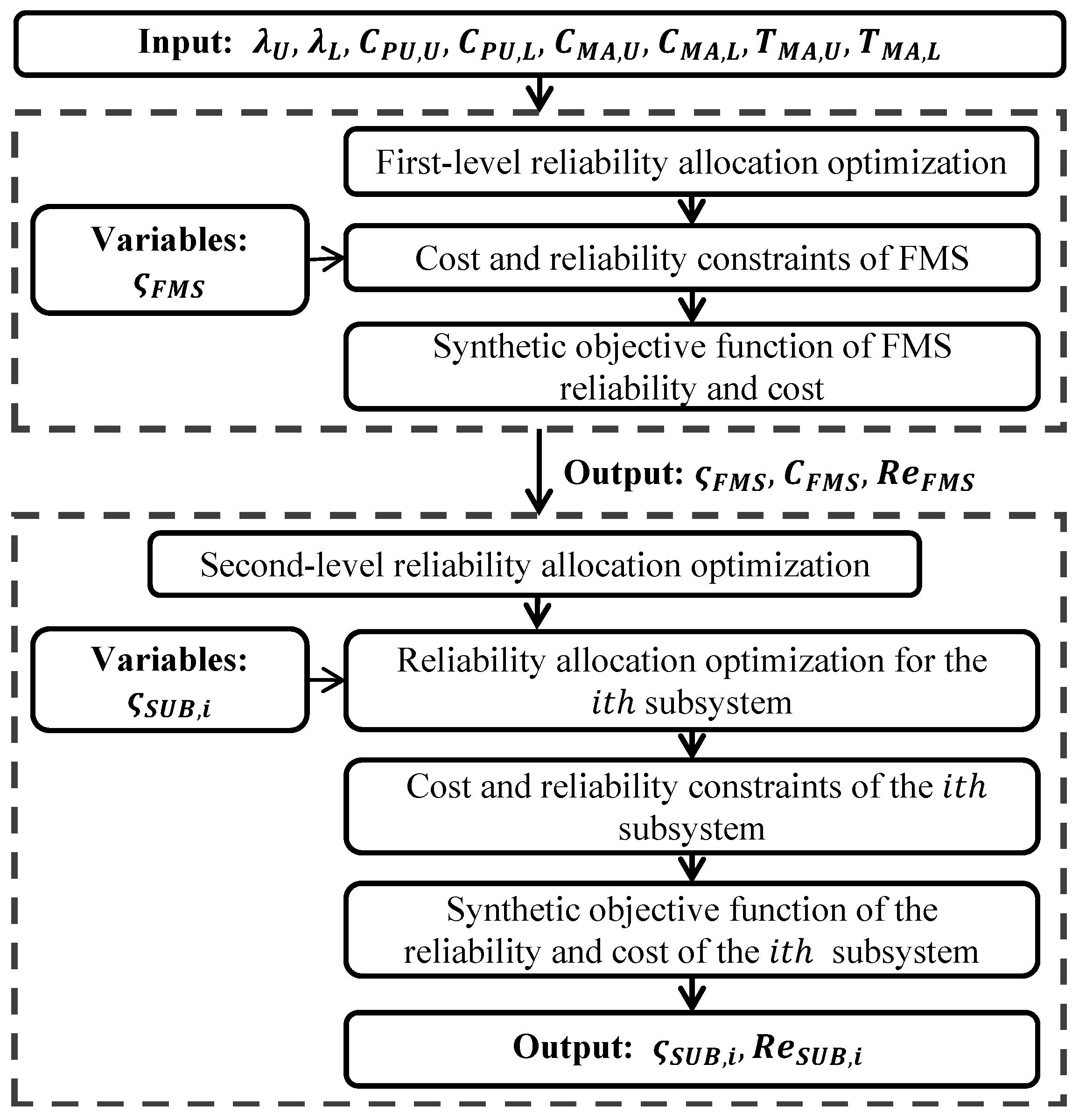
Based on BLOS, one overall optimization is transferred into several optimizations ( 1 + L ), L means the number of subsystems composed of several basic elements. These new optimizations have fewer variables. Among them, the number of variables of the first-level optimization is the same as the number of FMS subsystems, and the number of variables of each second-level optimization is the same as the number of basic elements of the corresponding subsystem. This strategy increases the number of optimizations but largely reduces the number of variables, and all subsystem optimizations can be processed in parallel, which can largely improve the optimization efficiency. The framework of the bi-level reliability-allocation optimization is shown in Figure 3, wherein λ U ,   λ L denote the vector composed of the upper limits and the vector composed of lower limits of the failure rate of all basic elements, respectively; C P U , U , C P U , L are the set of the upper limits and lower limits of the purchase fee of all basic elements, respectively; C M A , U , C M A , L are the vectors composed for the upper and lower limits of the maintenance fee of elements, respectively and T M A , U , T M A , L means the vectors composed of the upper and lower limits of the maintenance time of elements, respectively. The above values are the input of the optimization, which can be determined by expert experiences, production manuals, and the current technological level.

4.2. Bi-Level Optimization Algorithm Based on PSO

Based on PSO and BLOS, the pseudo-code of the bi-level reliability-allocation optimization algorithm is presented in Algorithm 2.
     
Algorithm 2: Optimization Algorithm Based on BLOS
  •      First-level optimization process:
  •      Initialize the variable set ς F M S , 0 ;
  •      PSO parameters setting N g , N p , ω , c 1 , c 2 , v m a x ;
  •      for i = 1 to Ng do
  •          for j = 1 to Np do
  •              Calculate the FMS cost C F M S ς F M S by Equation (9) and the FMS reliability R e F M S ς F M S when t = T by Equation (3);
  •              fpd,j = fFMS;
  •              if f p d , j > f j   C F M S ς F M S C t h r e d     R e F M S ς F M S R e t h r e d then
  •                  fpd,j = f(j); xpd,j = xj
  •              end if
  •          end for
  •          if f g d , i > min f p d then
  •               f g d , n u m = min f p d ; x g d = x p d , n u m
  •          end if
  •          Update the current flying velocities and positions of all particles by Equation (14);
  •      end for
  •      Calculate the reliability of the ith subsystem R e S U B , i ( ς S U B , i , o p t ) ;
  •      Calculate the cost of the ith subsystem C S U B , i ( ς S U B , i , o p t ) ;
  •      Second-level optimization process (for the ith subsystem):
  •      Initialize the variable set ς S U B , i , 0 ;
  •      PSO parameters setting N g , N p , ω , c 1 , c 2 , v m a x ;
  •      for i = 1 to Ng do
  •          for j = 1 to Np do
  •              Calculate the subsystem cost C S U B , i ( ς S U B , i ) by Equation (15) and the subsystem reliability R e S U B , i ( ς S U B , i ) when t = T by Equations (1) and (2);
  •              fpd,j = fLS;
  •              if f p d , j > f ( j )     C L S ( ς l s ) C L S ( ς L S , o p t )     R e L S ( ς l s ) R e L S ( ς L S , o p t ) then
  •                  fpd,j = f(j); xpd,j = xj
  •              end if
  •          end for
  •          if f g d , i > m i n ( f p d ) then
  •               [ f g d , n u m ] = m i n ( f p d ) ; x g d = x p d , n u m
  •          end if
  •          Update the current flying velocities and positions of all particles by Equation (14);
  •      end for

5. Application Case to a Box-Part Finishing FMS

5.1. Settings of the Application Case

In this section, the proposed optimization strategies are applied to a box-part finishing FMS, which is composed of one logistics subsystem and three machining lines. The machining line includes one marking machine, two pallet changers, one machine tool, one measuring machine, and one guided unloading robot. The box-part finishing FMS layout is shown in Figure 4, in which there exist 47 variables (that is, the reliability-level factors of all bottom elements including human, upper control system, station-level control systems of logistics subsystem, and three machining-line subsystems, mechanical and control systems of equipment of subsystems), and suppose that differences between three machining-line subsystems are ignored, the number of variables can be considered to be 21.
To perform the application, the setting for the failure rate, purchase fee, maintenance fee, and maintenance time of the bottom elements are listed in Table 2 and Table 3, wherein human failure means a mistake made by a human in the process of operation and the purchase fee of human means the expense incurred by employment. In this case, the FMS reliability is required no less than 0.85 when T = 2000   h (the FMS reliability can be calculated as 0.7281 when the failure rates of all bottom elements are taken as lower limit values and as 0.9565 while taking upper limit values). For ease of validation, it is assumed that the purchase fee, maintenance fee, and maintenance time of the bottom element are linearly related to the reliability-level factor (the specific correlation function can be determined based on expert experience and studies in real applications). Based on this assumption, the current values for these terms can be obtained by C P U ( ς ) = C P U , L + ς ( C P U , U C P U , L ) , C M A ( ς ) = C M A , L + ς ( C M A , U C M A , L ) , T M A ( ς ) = T M A , L + ς ( T M A , U T M A , L ) . And the threshold of the FMS cost is taken as 1700 (the FMS cost can be calculated as 1477.1 when reliability-level factors take lower limit values, and as 1939.3 when upper lower limit values are taken). In the following content, the results based on different optimization algorithms are compared to show the advantage of the proposed strategies through MATLAB simulations.

5.2. Validation of the RWTS-Based Algorithm

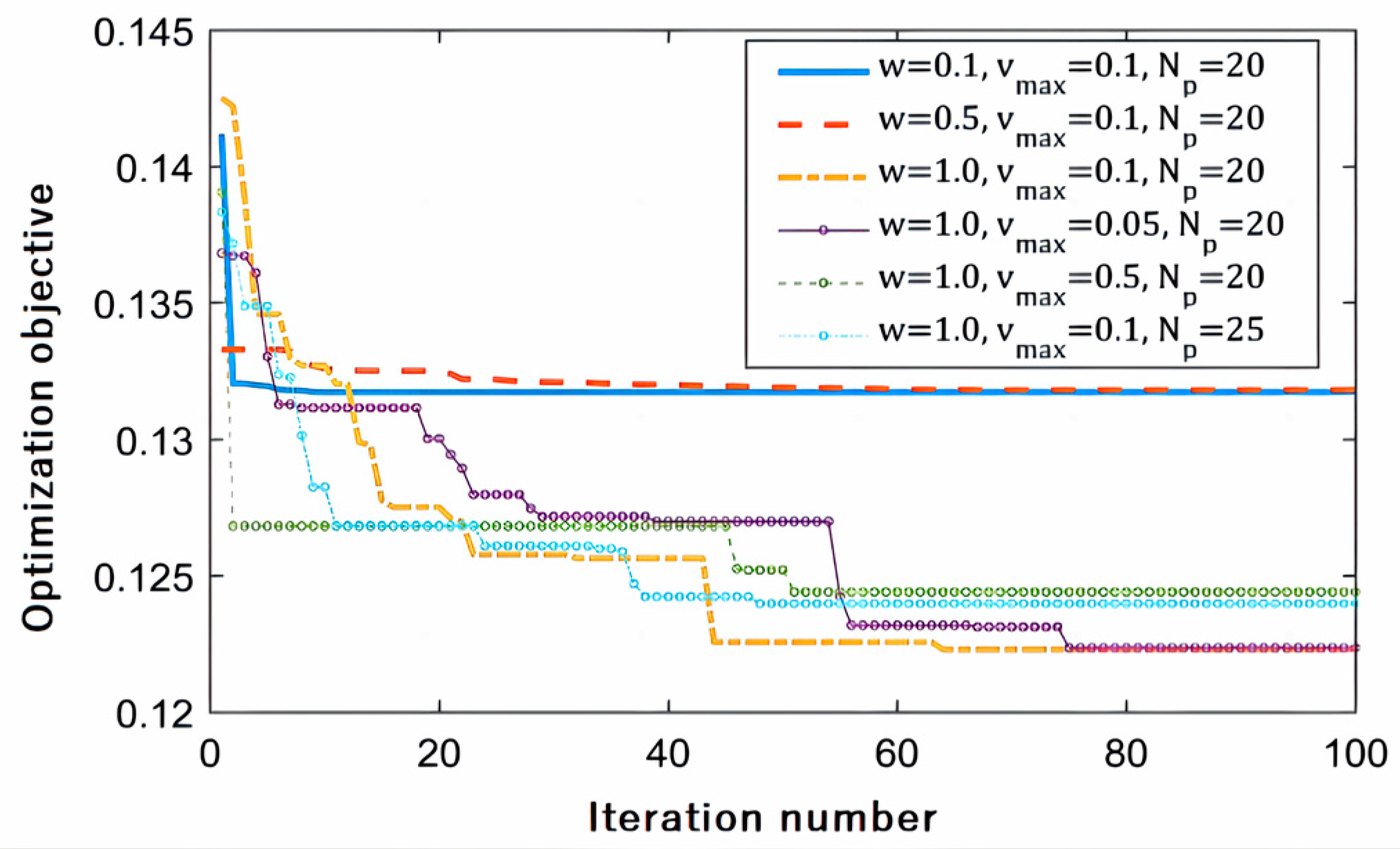
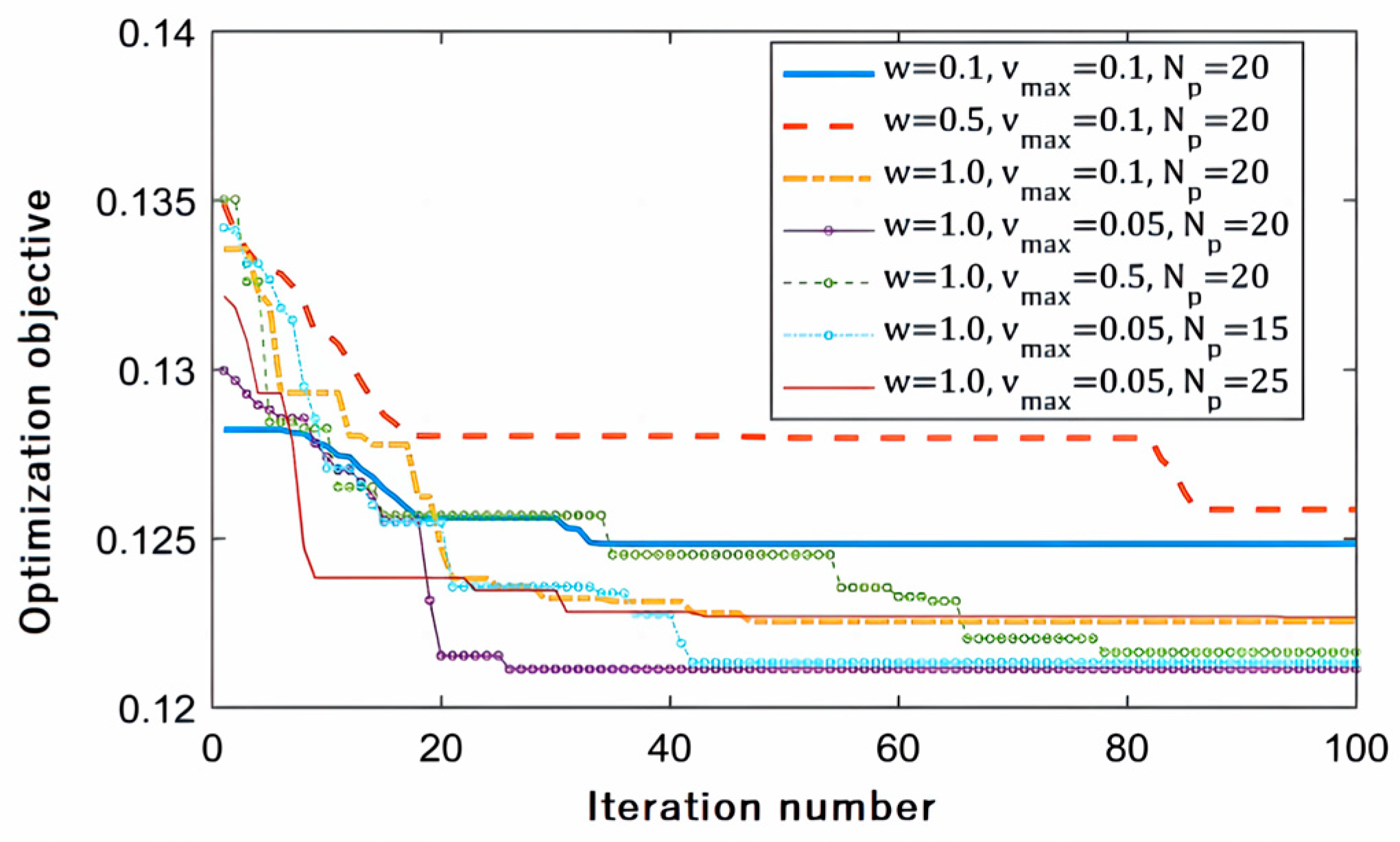
Since PSO parameters have a major impact on the optimization performance, the iteration curves of the optimization without RWTS (the general overall optimization) and that with RWTS are shown in Figure 5 and Figure 6, respectively. The optimal results based on two algorithms are also listed in Table 4, wherein for the reliability-level factors, the comparison value is calculated by Δ = x 1 x 2 , x 1 and x 2 denote their optimal result with RWTS and that without RWTS; for other parameters, the comparison value Δ is calculated by Δ = ( x 1 x 2 ) / x 2 × 100 % .
The main discussions and conclusions of the comparison are as follows:
(1) For the algorithm without RWTS, it converges at 0.1223 after 65 iterations when PSO parameters take w = 1.0 ,   v m a x = 0.1 ,   N p = 20 ; for the algorithm with RWTS, it converges at 0.1211 after 26 iterations when PSO parameters take w = 1.0 ,   v m a x = 0.05 ,   N p = 20 . The result indicates that both the convergence speed and optimization effect of the algorithm with RWTS are better than that without RWTS.
(2) From Table 4, compared with results without RWTS, the FMS reliability is improved by 0.67%, the optimization objective is reduced by 0.98%, and the convergence speed is increased by 54.15% (the convergence time is reduced from 68.7121 s to 31.5057 s), although the cost is increased by 0.14%. This comparison can also indicate that the proposed RWTS can largely improve the convergence speed.

5.3. Validation of the BLOS-Based Algorithm

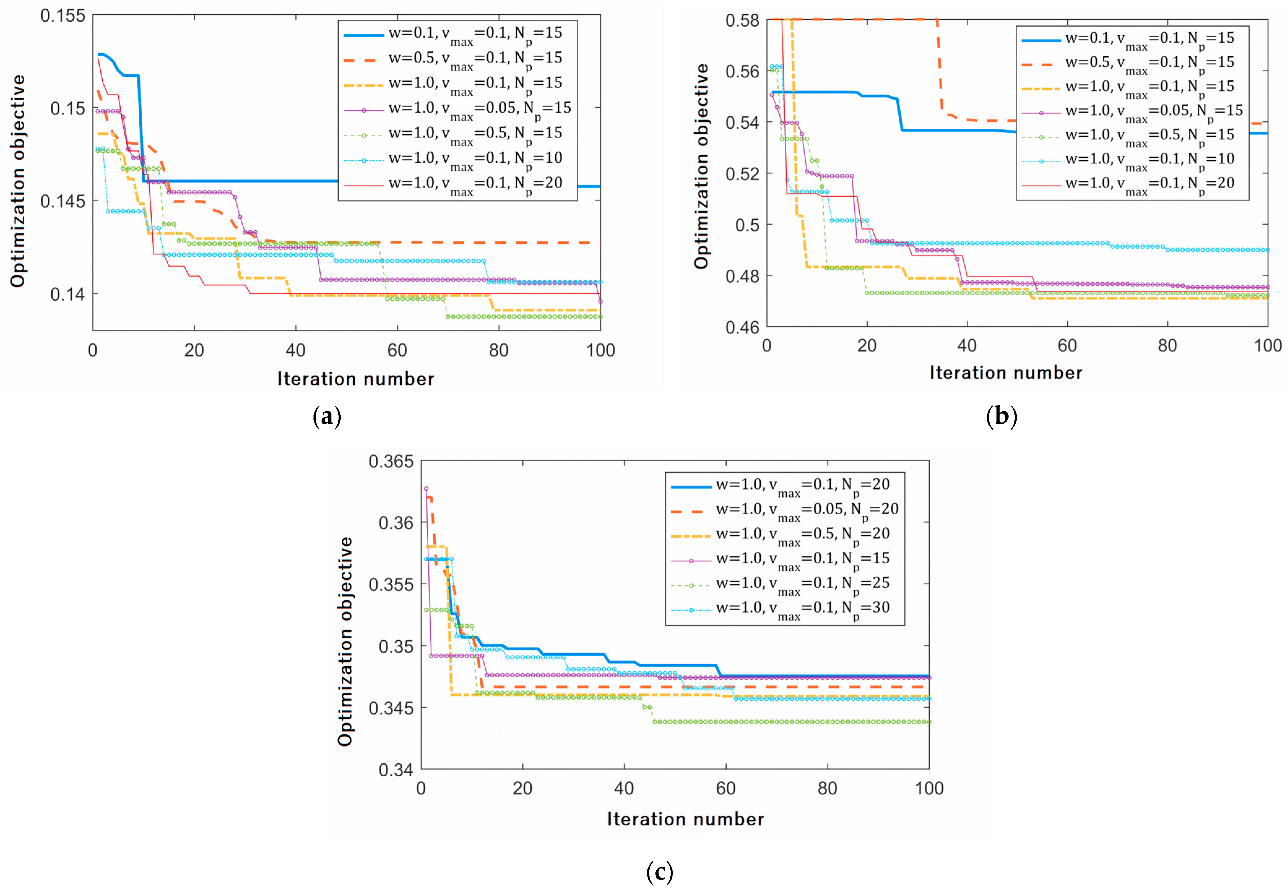
The iteration curves of the first-level and second-level algorithms are shown in Figure 7. The optimal results based on the BLOS-based algorithm are also listed in Table 5.
Compared the results of the bi-level optimization and the overall optimization (as listed in Table 4), the main discussions and conclusions are as follows:
(1) For the first-level algorithm, it converges at 0.1387 after 69 iterations when PSO parameters take w = 1.0 ,   v m a x = 0.5 ,   N p = 15 ; for the second-level optimization of the logistics subsystem, it converges at 0.4722 after 20 iterations when PSO parameters take w = 1.0 ,   v m a x = 0.5 ,   N p = 15 ; for the second-level optimization of the machining-line subsystem, it converges at 0.3438 after 46 iterations when PSO parameters take w = 1.0 ,   v m a x = 0.1 ,   N p = 25 . The convergence times of the three optimizations are 9.4294 s, 3.2501 s, and 10.8344 s. Compared with the convergence time of the overall optimization without RWTS (68.7121 s) and that with RWTS (31.5057 s), the total convergence time of the bi-level optimization (23.5139 s) is reduced by 65.78% and 25.37%, respectively, which means the convergence speed can be largely improved using BLOS.
(2) From the first-level optimization results of Table 5, the optimal cost and reliability of the logistics subsystem are 107.6 and 0.9324, and those of the machining-line subsystem are 358.7 and 0.6411, respectively. These values determine the threshold values for the cost and reliability of second-level optimizations. The values for these parameters obtained by the second-level optimizations satisfy the corresponding constraint thresholds determined by the first-level optimization. Moreover, based on the bi-level optimization strategy, the final optimal FMS cost and reliability can be calculated based on the optimal values of the reliability-level factors of all bottom elements, and they are 1683.4 and 0.9033, which satisfy their constraint thresholds of 1700 and 0.85, respectively. The above results show the effectiveness of the proposed optimization strategy.
(3) In the first-level and second-level optimizations, there is a small difference between the initial value of the reliability or cost and its corresponding optimal value, which means these sub-optimizations can be iterated quickly to obtain a solution that meets the constraints and is also close to the global optimal solution while taking the proper PSO parameters, indicating that the overall optimization efficiency can be effectively improved through the bi-level optimization strategy.

5.4. Overall Comparison of Four Algorithms

In this section, the FMS reliability-allocation optimization problem is solved by four algorithms, including the overall optimization algorithm based on RWTS (Algorithm 1), the optimization algorithm based on BLOS (Algorithm 2), the general overall algorithm (Algorithm 3), and the optimization algorithm based on RWTS and BLOS (Algorithm 4). Then, the convergence speed and optimization effect are compared to show the advantages of the proposed strategies. For ease of comparison, the number of iterations for convergence and the convergence time are taken when the values required when the optimization objective is first reduced to the minimum. Also, due to the process randomness of PSO optimization iterations, to consider the influence of this randomness on results, each algorithm was performed 10 times for the comparative analysis.
Figure 8 shows the comparison of convergence times of three algorithms, wherein M e a n denotes the average convergence time of 10 times optimization. From this figure, the convergence times of Algorithm 3 are significantly larger than that of other algorithms and are greatly affected by iterative randomness, while the convergence times of other methods are less affected by this randomness. Moreover, it shows that the average convergence time of Algorithm 4 is the smallest, which is 15.7473 s. Compared with Algorithm 1, Algorithm 2, and Algorithm 3, it is reduced by 38.03%, 23.95% and 76.01%, respectively.
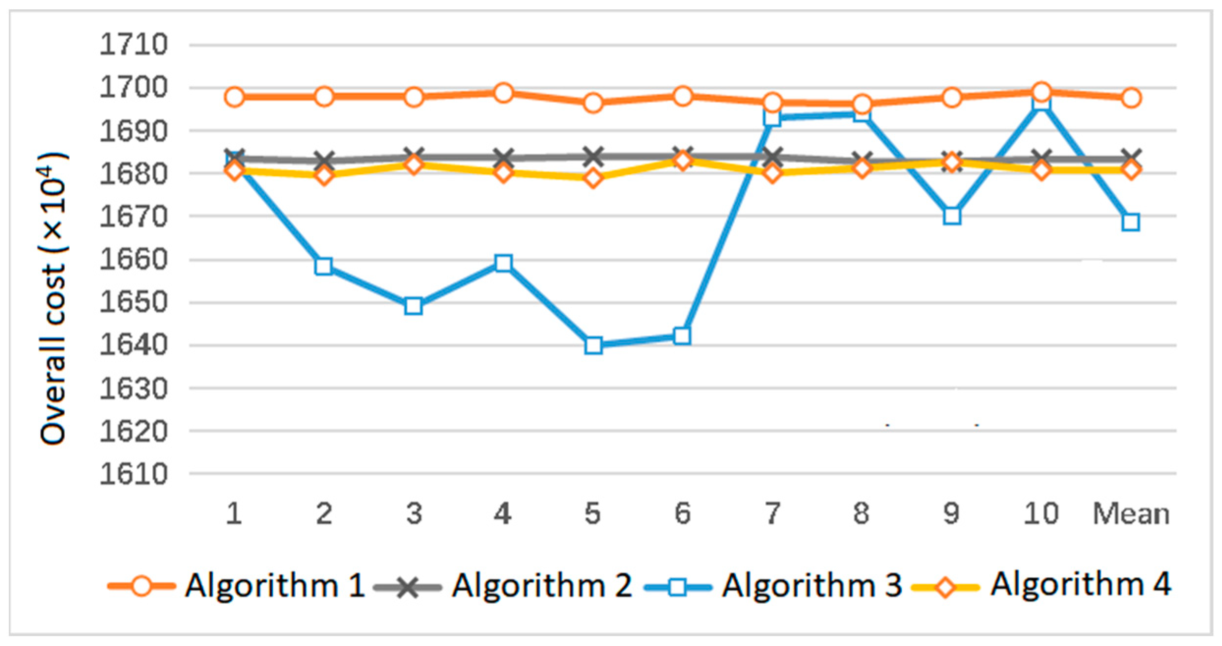
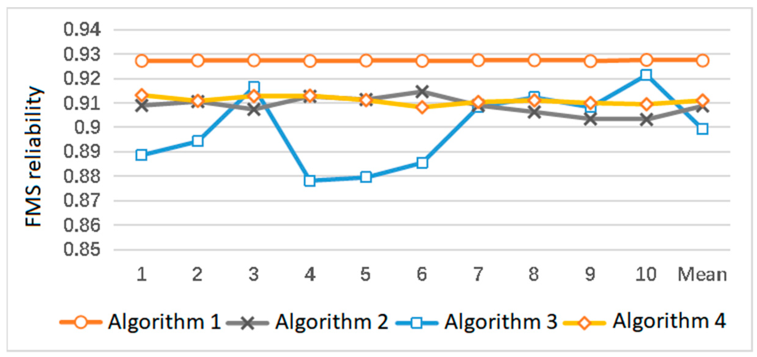
Figure 9 and Figure 10 show the comparison of the overall costs and FMS reliability values based on three algorithms. From these figures, the following main conclusions can be obtained.
(1) The cost and reliability of FMS based on Algorithm 3 are greatly affected by iteration randomness. The cost variance and reliability variance of the results of 10 times optimization are 20.7937 and 0.0151, respectively. Other algorithms are less affected, with cost variances of 0.9149, 0.4361, and 1.2615, and reliability variances of 0.0001, 0.0035, and 0.0015, respectively, among which Algorithm 1 is the least affected.
(2) On average, the FMS cost based on Algorithm 1 is higher than that based on other algorithms, which is 0.84% and 0.99% higher than that of Algorithms 2 and 4, respectively, but the reliability of FMS is also significantly higher than that of other algorithms, which is 2.05% and 1.79% higher than that of Algorithms 2 and 4, respectively.
(3) Compared with Algorithms 1 and 2, it shows that although both strategies of RWTS and BLOS can improve the convergence speed, BLOS can obtain higher reliability at less cost. The difference between cost and reliability averages based on Algorithms 2 and 4 is small and is 0.14% (for cost) and 0.25% (for reliability), respectively.
(4) Combined with the convergence time of Figure 7, the results indicate that the application of the proposed RWTS and BLOS can effectively improve the convergence speed and optimization effect.

6. Conclusions and Future Works

6.1. Conclusions

This work proposed two dimension-reduction strategies (RWTS and BLOS) to improve the optimization efficiency and effect for the reliability-allocation optimization problem of FMS. The overall optimization model and algorithm based on RWTS, as well as the bi-level optimization model and algorithm based on BLOS, are presented in detail. To show the advantages of the proposed strategies, an application case to a box-part finishing FMS is used in the simulation experiment. Finally, the comparisons of results obtained by the algorithm without strategies and algorithms with RWTS or BLOS are shown and discussed. The main conclusions are as follows:
(1) Compared with the general optimization method, the adoption of both strategies, RWTS and BLOS, can largely improve the optimization efficiency, guarantee that the optimal results meet the preset cost and reliability constraints, and effectively balance the cost and reliability requirements of FMS. The use of RWTS has a higher convergence speed than BLOS.
(2) From the comparison results of four algorithms, the use of RWTS has a higher convergence speed than using BLOS, and the use of both two strategies at the same time has a higher convergence speed than using one of them. Moreover, the use of strategies RWTS or BLOS can largely reduce the influence of the optimization iterative randomness on the convergence speed and optimal results, and although there are some differences in the reliability-level factors of elements optimized by four algorithms, they all achieve the effective improvement of FMS optimization objectives and can meet the cost and reliability constraints of FMS.
(3) The proposed method can be effectively used to balance the reliability and cost indexes during the reliability allocation of FMS, which is performed with the reliability and cost levels of elements as input, with quantitative models of the cost and reliability of FMS as the basis. The optimal results can provide an effective data basis for the system design or reconstruction.

6.2. Future Works

The proposed method was only validated by the simulation case. In future works, we will further seek cooperation with enterprises and use this method in the reliability design of the real FMS to show the engineering value of this work and continuously improve the method in practice. Moreover, we will develop software modules based on methods of reliability evaluation and reliability allocation to assist enterprises in better designing and optimizing the reliability of their manufacturing systems with limited capital support.

Author Contributions

Conceptualization, J.X.; Methodology, validation, and writing—original draft preparation, L.T. and Y.P.; Writing—review and editing, all authors; Supervision, Z.L. and Q.C.; Project administration, J.X.; Funding acquisition, J.X. and Z.L. All authors have read and agreed to the published version of the manuscript.

Funding

This work was supported by the National Key R&D Program of China (2022YFB3402800), R&D Program of Beijing Municipal Education Commission (No. KM202210005031), and the National Natural Science Foundation of China (No. U23B20104, No. 52105170).

Data Availability Statement

Data is contained within the article.

Conflicts of Interest

The authors declare no conflict of interest.

References

  1. Zhang, W.; Ran, Y.; Zhang, G.; Shao, Y. Optimal allocation of product reliability using novel multi-population particle swarm optimization algorithm. Proc. Inst. Mech. Eng. Part C J. Mech. Eng. Sci. 2022, 236, 4565–4576. [Google Scholar] [CrossRef]
  2. Zhou, C. Research on Evaluation, Prediction and Distribution of Reliability Index of Industrial Robot. Ph.D. Thesis, Hebei University of Technology, Tianjing, China, 2022. [Google Scholar]
  3. Liang, K.W. Reliability Engineering; National Defense Industry Press: Arlington, VA, USA, 2014. [Google Scholar]
  4. You, M.Y.; Zheng, J.C. A multi-source information based generalized proportional combination approach to reliability allocation of electronic systems. Electron. Prod. Reliab. Environ. Test. 2011, 29, 15–21. [Google Scholar]
  5. Shi, C.; Chen, Y. Basic reliability distribution of a new ship steering control system based on scoring method. Ship Electron. Eng. 2021, 41, 115–118. [Google Scholar]
  6. Wu, J.; Yang, Y.; Wang, Z. Research on the reliability allocation method of micro-robot based on combined weight. Manuf. Autom. 2022, 44, 93–97. [Google Scholar]
  7. Du, Y.; Wu, G.; Tang, Y.; Cao, H.; Liu, S. Reliability Allocation Method for Remanufactured Machine Tools Based on Fuzzy Evaluation Importance and Failure Influence. Int. J. Precis. Eng. Manuf.-Green Technol. 2021, 8, 1617–1628. [Google Scholar] [CrossRef]
  8. Abbas, S.; Hassan, Z. Use of ARINC Approach method to evaluate the reliability assignment for mixed system. J. Phys. Conf. Ser. 2021, 1999, 012102. [Google Scholar] [CrossRef]
  9. Qian, Y.; Jiang, C.; Su, L. Research of Reliability Allocation Based on Gray Theory. IOP Conf. Ser. Mater. Sci. Eng. 2021, 1043, 022006. [Google Scholar] [CrossRef]
  10. Neha; Verma, V.; Tandon, A.; Aggarwal, A.G. Software reliability allocation incorporating Pythagorean fuzzy theory and AHP. Int. J. Ind. Syst. Eng. 2021, 38, 19–34. [Google Scholar] [CrossRef]
  11. Feng, Y.K.; Chen, X.W.; Li, H.B.; Hu, N.; Ge, Z.J. Object-oriented programming design of dynamic planning method of reliability allocation. Electron. Prod. Reliab. Environ. Test. 2019, 37 (Suppl. S1), 106–112. [Google Scholar]
  12. You, M.N.; Luo, R.X. Study on reliability of supply chain collaborative product development based on dynamic planning. Logist. Technol. 2017, 36, 158–161. [Google Scholar]
  13. Zeng, L.; Zhu, Z.D.; Zhang, F.; Dai, M.; Yang, J. Redundancy reliability optimization of electro-hydraulic control system of ball screw actuators based on dynamic programming method. J. Xuzhou Inst. Technol. (Nat. Sci. Ed.) 2018, 33, 6–13. [Google Scholar]
  14. Wu, X.Y. Importance Based Reliability Allocation Modelling and Algorithm for Phased Mission System. Master’s Thesis, National University of Defense Technology, Changsha, China, 2018. [Google Scholar]
  15. Arezki, M.M.; Abdellah, S. System reliability-redundancy allocation by the multiobjective plant propagation algorithm. Int. J. Qual. Reliab. Manag. 2022, 39, 902–909. [Google Scholar]
  16. Kang, R.; Liu, H.R.; Zhang, Q.Y.; Yu, L.; Zhai, G.F. Function oriented belief reliability design and optimization of new torsion spring electrical connectors. J. Beijing Univ. Aeronaut. Astronaut. 2022, 48, 1745–1756. [Google Scholar]
  17. Pei, Y.; Liu, Z.; Xu, J.; Qi, B.; Cheng, Q. Grouping Preventive Maintenance Strategy of Flexible Manufacturing Systems and Its Optimization Based on Reliability and Cost. Machines 2023, 11, 74. [Google Scholar] [CrossRef]
  18. Sun, J.S. Research on Evaluation Index System for Patents Stratification in Universities. Master’s Thesis, Dalian University of Technology, Dalian, China, 2017. [Google Scholar]
  19. Xu, J.J.; Liu, Z.F.; Zhao, Y.S.; Pei, Y.; Cheng, Q. A path optimization technique with obstacle avoidance for an 8-dof robot in bolt looseness detection task. Int. J. Precis. Eng. Manuf. 2019, 20, 717–735. [Google Scholar] [CrossRef]
  20. Kim, H.J.; Kang, H.J.; Kim, M.K. Data-Driven Bidding Strategy for DER Aggregator Based on Gated Recurrent Unit-Enhanced Learning Particle Swarm Optimization. IEEE Access 2021, 9, 66420–66435. [Google Scholar] [CrossRef]
Figure 1. Framework of the proposed method, wherein the detailed description of the three-layer reliability evaluation index system can be found in reference [17].
Machines 12 00024 g001
Figure 2. Iteration process of the optimization based on RWTS.
Machines 12 00024 g002
Figure 3. Framework of the bi-level reliability-allocation optimization.
Machines 12 00024 g003
Figure 4. FMS layout of the application case.
Machines 12 00024 g004
Figure 5. Iteration curves without RWTS.
Machines 12 00024 g005
Figure 6. Iteration curves with RWTS.
Machines 12 00024 g006
Figure 7. Iteration curves of the first-level and second-level optimizations. (a) For the first-level optimization; (b) For the second-level logistics subsystem optimization; (c) For the second-level machining-line subsystem optimization.
Machines 12 00024 g007
Figure 8. Curves of the convergence time of four algorithms, wherein Algorithm 1 is the overall optimization algorithm based on RWTS, Algorithm 2 is the optimization algorithm based on BLOS, Algorithm 3 is the general overall algorithm, and Algorithm 4 is the optimization algorithm based on RWTS and BLOS.
Machines 12 00024 g008
Figure 9. Curves of the overall cost based on four algorithms, wherein Algorithm 1 is the overall optimization algorithm based on RWTS, Algorithm 2 is the optimization algorithm based on BLOS, Algorithm 3 is the general overall algorithm, and Algorithm 4 is the optimization algorithm based on RWTS and BLOS.
Machines 12 00024 g009
Figure 10. Curves of the FMS cost based on four algorithms, wherein Algorithm 1 is the overall optimization algorithm based on RWTS, Algorithm 2 is the optimization algorithm based on BLOS, Algorithm 3 is the general overall algorithm, and Algorithm 4 is the optimization algorithm based on RWTS and BLOS.
Machines 12 00024 g010
Table 1. Three-level reliability evaluation index system.
WLSSLEL
R e F M S R e H U M A N
R e U C
R e L C S
R e L S R e L S , R O B ,   R e L S , R O B C ,   R e L S , C A R ,   R e L S , C A R C , R e L S , B U F
R e M C S , m ,   1 m M
R e M S , m ,   1 m M R e M S , M A C , m n ,   R e M S , M A C C , m n ,   1 n N
Table 2. Failure rates of reliability evaluation factors of the box-part finishing FMS (UCS: upper control system; SLCS-LS: station-level control system for logistics subsystem; SLCS-MS: station-level control system for machining-line subsystem; LR(ULR): loading robot (unloading robot); LC: logistics car; MM: marking machine; PC: pallet changer; MT: machine tool; ME: measuring machine; XX_MS and XX_CS: mechanical system and control system of one equipment XX).
Elements λ L ~ λ U ( h 1 )Elements λ L ~ λ U ( h 1 )
HUMAN 1 ~ 5   ( × 10 6 ) MMMM_MS 1 ~ 5   ( × 10 4 )
UCS 5 ~ 10   ( × 10 5 ) MM_CS 1 ~ 5   ( × 10 5 )
SLCS-LS 1 ~ 5   ( × 10 5 ) PCPC_MS 5 ~ 20   ( × 10 5 )
SLCS-MS 1 ~ 5   ( × 10 5 ) PC_CS 1 ~ 5   ( × 10 5 )
LR (ULR)LR(ULR)_MS 2 ~ 10   ( × 10 5 ) MTMT_MS 2 ~ 8   ( × 10 4 )
LR(ULR)_CS 1 ~ 5   ( × 10 5 ) MT_CS 1 ~ 5   ( × 10 5 )
LCLC_MS 5 ~ 20   ( × 10 5 ) MEME_MS 1 ~ 5   ( × 10 4 )
LC_CS 1 ~ 5   ( × 10 5 ) ME_CS 1 ~ 5   ( × 10 5 )
Buffer zone 5 ~ 10   ( × 10 6 ) --
Table 3. Setting of purchase fee, maintenance fee, and maintenance time of the bottom elements.
Elements C P U , L (RMB) C P U , U (RMB) C M A , L (RMB) C M A , U (min) T M A , L (min) T M A , U (min)
HUMAN24,00030,0000000
UCS80,000100,0008001000150180
SLCS-LS50,000100,0005001000100120
SLCS-MS300,000500,00030005000500600
XX_CS30,00050,0003005006080
LR(ULR)_MS200,000300,00020003000400500
LC_MS50,000100,0005001000150200
MM_MS300,000500,00030005000250300
PC_MS150,000200,00015002000200240
MT_MS1,500,0002,000,00015,00020,0008001000
ME-MS350,000500,00035005000300400
Table 4. Optimal results based on two algorithms, wherein ς i means the reliability-level factor of the i t h bottom element.
ParametersResults with RWTSResults without RWTS
Comparison   Value     or  
Initial ValueOptimal ValueInitial ValueOptimal Value
ς 1 0.92690.88950.27330.18570.7038
ς 2 0.27200.98030.83661−0.0197
ς 3 0.394410.43080.98180.0182
ς 4 0.24410.01750.91030.5574−0.5399
ς 5 0.73980.66320.21920.55520.108
ς 6 0.91290.99670.86470.94440.0523
ς 7 0.03760.93130.02090.72060.2107
ς 8 0.27850.36400.45210.22330.1407
ς 9 0.85020.90380.20531−0.0962
ς 10 0.03600.28980.28160.3044−0.0146
ς 11 0.659600.99230.3833−0.3833
ς 12 0.508000.10070.4412−0.4412
ς 13 0.630200.68850.1045−0.1045
ς 14 0.57320.83390.04900.56150.2724
ς 15 0.077200.10570.7115−0.7115
ς 16 0.549000.81550.4152−0.4152
ς 17 0.801400.72690.7352−0.7352
ς 18 0.50600.88490.14890.70040.1845
ς 19 0.202900.04900.9433−0.9433
ς 20 0.576500.59390.0288−0.0288
ς 21 0.695300.07010.6211−0.6211
C F M S ( × 10 4 ) 1694.81699.11617.21696.70.14%
R e F M S 0.89160.92770.85670.92150.67%
f 0.13890.12110.15250.1223−0.98%
Convergence time(s) 31.5057
(After 26 iterations)
68.7121
(After 65 iterations)
54.15%
Table 5. Optimal results based on the BLOS-based algorithm, wherein ς L S and ς M S are the reliability-level factors of the logistics subsystem and the machining-line subsystem, respectively; ς L S , i means the reliability-level factor of the i t h bottom element of the logistics subsystem; ς M S , i means the reliability-level factor of the i t h bottom element of the machining-line subsystem.
First-Level OptimizationSecond-Level Optimizations
ParametersInitial ValueOptimal ValueParametersInitial ValueOptimal Value
ς H U M A N 0.67080.3632 ς L S , 1 0.75570.5222
ς U C S 0.87941 ς L S , 2 0.66161
ς S L C S L S 0.41111 ς L S , 3 0.99711
ς S L C S M S 0.47071 ς L S , 4 0.19870.0190
ς L S 0.97950.8114 ς L S , 5 0.53390
ς M S 0.12380.2692 C L S ( × 10 4 ) 105.387.9
C F M S ( × 10 4 ) 1627.21696.5 R e L S 0.93250.9345
R e F M S 0.85770.8921 f L S 0.56000.4722
f F M S 0.15250.1387Convergence time(s) 3.2501 (After 20 iterations)
C L S , o p t 107.6 ς M S , 1 0.19070.2627
R e L S , o p t 0.9324 ς M S , 2 0.15260.1327
C M S , o p t 358.7 ς M S , 3 0.36040.3086
R e M S , o p t 0.6411 ς M S , 4 0.02210.2575
Convergence time(s)9.4294 (After 69 iterations) ς M S , 5 0.27580.2640
---- ς M S , 6 0.36810.0688
---- ς M S , 7 0.15290.4675
---- ς M S , 8 0.09230.2179
---- ς M S , 9 0.30380.6188
---- ς M S , 10 0.46790.0705
---- ς M S , 11 0.13300
---- ς M S , 12 0.06050
---- C M S ( × 10 4 ) 353.9357.6
---- R e M S 0.64820.6700
---- f M S 0.35280.3438
----Convergence time(s) 10.8344 (After 46 iterations)
Disclaimer/Publisher’s Note: The statements, opinions and data contained in all publications are solely those of the individual author(s) and contributor(s) and not of MDPI and/or the editor(s). MDPI and/or the editor(s) disclaim responsibility for any injury to people or property resulting from any ideas, methods, instructions or products referred to in the content.