Abstract
The multi-random-effects gamma process has a better characterization effect for degraded data with individual differences. In this paper, a reliability evaluation method for gamma stochastic processes with multiple random effects is studied. The mathematical model of multiple random effects gamma process was established. The model parameters estimation method was established based on the Bayesian approach. The prior distribution acquisition method was discussed, and the parameters of the multiple randomeffects gamma process were estimated by the MCMC-Gibbs method. The correctness of the model and method was verified by numerical simulation, the influence of algorithm parameters on the algorithm solving process was studied. In the fourth part, the reliability of aviation hydraulic rotary joints was studied by using multiple random effects gamma processes.
1. Introduction
Nowadays, the reliability of products is a focus issue in the product manufacturing industry. Under the impact of external and internal stress, the physical or chemical changes in the materials of the product will lead to the gradual degradation of product performance. When the performance degrades to the specified threshold, the products will be considered to be in a failed state. This type of failure is called soft failure, which is a primary failure mode of products. The performance degradation data of the products contain past and current health status information, and the future health status of the products can be evaluated based on this information. The remaining service life and operation reliability of the products can be predicted according to the performance degradation information, which can provide scientific guidance for product maintenance, repair and replacement [1,2,3,4,5].
It is important to select a suitable degradation model to describe the process of product performance degradation. The traditional mathematical model was first used in reliability evaluation and residual life prediction. Before the 1990s, the simple regression model was used as a degradation process model to describe the product performance degradation process. However, the simple stochastic model could not take the uncertainty in the model of product performance degradation, so the remaining life value obtained by the model is a definite value, which is not consistent with the actual situation. Later, Lu and Meeker [6] proposed a stochastic coefficient regression model for the product performance degradation process. The regression coefficient is considered as a random parameter, and the measurement noise item is added to the model. Then the model has been developed to some extent. Wang et al. [7] summarized the stochastic coefficient regression model and calculated the failure threshold by optimization method. The random time series model is also applied to product life prediction.
The stochastic process model is an important degradation model, which is widely used to describe the degradation process of product performance because of its good mathematical characteristics. The Wiener process is the earliest stochastic process introduced into the reliability field [8,9,10,11,12]. Afterward, the inverse Gaussian process [13,14,15] and the gamma process are also used as mathematical models for different degradation processes.
The gamma process can be used to describe wear, aging and fatigue phenomena. In recent years, the theoretical research of gamma processes has been developed rapidly and has been widely used in the field of engineering reliability. Duan et al. [16] studied the design problem of the step-stress accelerated degradation test (SSADT) based on the non-stationary gamma process with random effects. Mercier et al. [17] analyzed two imperfect repair models for a degrading system; the deterioration level of the system was modeled by a nonhomogeneous gamma process. This study provides a reference for the maintenance of the system. Ling et al. [18] studied the degradation analysis for products with two-phase degradation under gamma processes. The research proposed a Bayesian approach and a likelihood approach via a stochastic expectation-maximization algorithm for the statistical inference of the remaining useful life. Cholette et al. [19] used gamma processes to study the performance degradation process of boiler heat exchanger. Jiang et al. [20] proposed a Gamma constant-stress accelerated degradation model based on the principle of the degradation mechanism invariance. Paroissin [21] built a recursive estimator using an online estimation problem for gamma processes. Song et al. [22] proposed a time-discrete and zero-adjusted gamma process model. The results show that the proposed model has satisfactory fit performance and predictive performance. Fan et al. [23] used the gamma processes model to predict the real lumen decay and color shift lifetimes. Wang et al. [24] used Gamma processes to predict the lifetime based on accelerated degradation data. Lin et al. [25] presented a two-phase gamma process model, and the model was applied to estimate the state of charge and the remaining useful discharge time of batteries. Wang et al. [26] proposed a dynamic RUL prediction and optimal maintenance time (OMT) determination approach using a Gamma process model. Salem et al. [27] studied parameter estimation and lifetime prediction of differential gamma processes.
The Gamma degradation model with random effects has a good fitting effect for the degenerate data, which was researched in the literature [28,29,30,31]. Zhou et al. [32] proposed a reparameterized gamma process with random effects; the variational Bayesian algorithm was used to infer the model parameters. The results show that the proposed method is superior to MCMC algorithm and EM algorithm in computational efficiency and estimation accuracy.
The multi-random-effects gamma process has a better characterization effect for degeneration data with individual differences. In previous studies, the scale parameter of the gamma process was often taken as random parameters, and the randomness of the initial values was not considered. In order to further expand the reliability evaluation method based on gamma processes, this paper proposes a reliability evaluation method for gamma stochastic processes with multiple random effects. The model takes into account the randomness of the initial value and degradation rate, and adopts the distribution of random parameters different from previous studies. In the first part, the mathematical model of the multi-random-effects gamma process was established. In the second part, the model parameters estimation method was established based on the Bayesian approach. The prior distribution acquisition method was discussed, and the parameters of the multi-random-effects gamma process were estimated by the MCMC-Gibbs method. In the third part, the correctness of the model and method was verified by numerical simulation. In the fourth part, the reliability of aviation hydraulic rotary joints was studied by using multi-random-effects gamma processes. This method has certain theoretical significance and engineering application value.
2. Mathematical Model of Multiple Random Effects Gamma Processes
2.1. Gamma Random Process
The gamma process is a classic random process with independent and non-negative increments, which is suitable for representing degradation phenomenon characteristics such as crack growth and metal wear. The degradation value of the sample at time is represented by . The gamma process satisfies the following characteristics:
(1) For any moment , the degradation increment is independent.
(2) The degenerate increment beys the Gamma distribution , where is the scale parameter and is the monotonically increasing shape parameter.
If , the probability density function of the gamma distribution is:
where is the shape parameter and is the scale parameter, is a gamma function.
2.2. Multiple Random Effects Gamma Processes
The initial value of equipment performance degradation value is inconsistent due to environmental change, manufacturing error and installation technology in the manufacturing process. Moreover, in the work process, the random stress and the difference in equipment material properties lead to a dynamic and random fluctuation of equipment performance degradation rate. In order to improve the accuracy of reliability assessment, the model should be further improved.
When considering the influence of random effects on the gamma process, the initial value and the degradation rate are random, and the difference between the initial value and the degradation rate will affect the remaining life prediction accuracy. Therefore, in order to describe the degradation process more accurately, the randomness of the degradation process should be considered.
Considering that the degradation process of product performance changes with time, assuming that the degradation process conforms to the change law of gamma process, the degradation amount of equipment at any time can be described by the following model:
where is the initial value of degradation parameter value, is the gamma process with shape parameter and scale parameter .
It is reasonable to assume that the distribution of initial parameters is uniform when certain dimensional tolerances need to be satisfied during manufacturing. Assuming a uniform distribution .
Parameters and can be used as influencing parameters of degradation rate. In this paper, the shape parameter is regarded as a random parameter to describe the difference of degradation rate. When the shape parameter is selected as a linear function , it is assumed that the distribution followed by the parameter is uniform distribution, .
3. Parameter Estimation of Degradation Model Based on Bayesian Method
3.1. Bayesian Parameter Estimation
Based on Bayesian statistical theory, the Bayesian approach is an important method of parameter estimation, which has been widely used in reliability engineering [33]. Bayesian approach considers the function of prior information of the unknown parameters in the process of parameter estimation and combines the available data with prior information. Bayesian approach treats the unknown parameters as random variables and obtains the posterior distribution of the unknown parameters according to the following formula:
where is the prior density function of the parameter . is the conditional density function under known parameter , which is called the likelihood function.
It is assumed that there are a total of samples for the test, and each sample has been measured () times during the test. Note that the degradation amount measured at the second measurement time of the second sample is , the two adjacent measurement intervals are , and the degradation increment between the two adjacent measurement intervals is . According to the characteristics of gamma distribution, the degradation increment is satisfied.
Assuming that the samples are independent of each other, , the likelihood function for the random effect gamma process is expressed as:
where is a random variable subject to uniform distribution, and the probability density function is:
After obtaining the probability density function of the parameter based on Formula (3), the Bayesian estimation of the parameter under the square loss function is:
The computation of posterior distribution for based on Formula (3) is an intractable problem bottleneck in Bayesian analysis. When faced with complex high-dimensional problems, it is difficult to obtain a posterior distribution through analytical methods. MCMC (Markov Chain Monte Carlo) and EM algorithm are two commonly used algorithms in Bayesian formula parameter estimation. MCMC is based on the Markov theory and Monte Carlo method, which directly simulates independent random samples of the posterior distribution, and then obtains the relevant statistical characteristic information values by analyzing the simulated samples. In this paper, MCMC method is used to estimate the unknown parameters of the model.
This paper proposes a reliability estimation method, as shown in Figure 1. Firstly, the unknown parameters of the gamma process are estimated by using the moment method based on the degradation data. The prior distribution of unknown parameters of multi-random effect gamma processes is constructed according to the estimated results of unknown parameters. Then, based on the degradation data and the prior distribution of unknown parameters, the MCMC method is used to estimate the unknown parameters of the multi-random effects gamma process, and the multi-random effects gamma process model is obtained. Finally, the life distribution was obtained by Monte Carlo method.
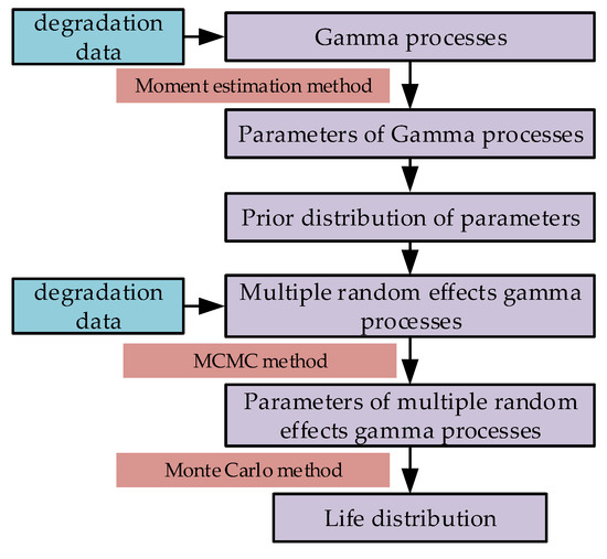
Figure 1.
Method flow.
3.2. Determination of the Prior Distribution
The prior information can be utilized in the Bayesian method, so the probability distribution form and parameters in the Bayesian model should be obtained according to experience and historical data. Uniform distribution and gamma distribution are the common distribution types used as prior distributions. When prior information is insufficient, gamma distribution is the most commonly used distribution. In this paper, uniform distribution and gamma distribution are used as prior distributions, and the method of obtaining parameters of uniform distribution is studied.
There are a total of degenerate samples. For each degenerate sample, , ,. The sample mean and sample variance of each degenerate sample can be calculated as:
The estimated values of parameters and can be obtained as:
The estimated values of parameters and can be obtained. According to the estimated values of parameters and of each degradation curve, the corresponding distribution types and parameters can be constructed.
The distribution test method can be used to select and analyze the random distribution types of model parameters. Therefore, the distribution types of model parameters can be determined whether they conform to the set distribution types. Due to the randomness of the degenerate process, the parameters and in the gamma process are stochastic. When the gamma process parameters are taken as a random parameter, one of the parameters is generally regarded as a random parameter. Therefore, when distribution test for random parameters are conducted, another parameter is treated as a fixed parameter. It can improve the accuracy of parameter distribution test. For example, if the parameter is regarded as a random parameter, the estimated value parameter for the distribution test can be calculated as follows:
where is the mean value of calculated by Formula (13).
When the prior distribution cannot be obtained, conjugate distribution is often used as the distribution type of the prior distribution. For the random parameters of a gamma process, the gamma distribution can be used as a prior distribution. However, it is difficult to obtain the value of the prior distribution parameters, and the prior distribution parameters have an important effect on the parameter estimation result.
The parameter estimation values of each curve are calculated according to Equations (12) and (13). For parameter , when parametric randomness is described by uniform distribution, the parameter and need to be obtained. Either a uniform distribution or a gamma distribution can be used as a prior distribution. However, the parameters of the gamma distribution are difficult to obtain. When the uniform distribution is used as the prior distribution, the parameter values of the prior distribution are most likely to be located near the minimum and maximum of the moment estimation value of parameter . The parameters of the prior distribution can be constructed using the minimum and maximum of the moment estimation value, which are discussed in Section 4.2.1. For parameter , When a uniform distribution is used as a prior distribution, the values of the prior distribution can be taken using the maximum and minimum values of the parameter moment estimation value.
3.3. Life Distribution Prediction Process
When the performance degradation value reaches the failure threshold, it means that the product performance is seriously deteriorated: even if it is working normally, it is regarded as failure. The service life of the product is the time from the product come into use to the first time it reaches the failure threshold.
Therefore, the service life of the product is defined as:
where is the failure threshold.
When the parameters of degradation model are fixed effect parameters, the probability density function and distribution function of failure time are:
where .
When considering the uncertainty of initial values and degenerate parameters, , let replace , the probability density function and distribution function of the available failure time are:
The probability density function and distribution function of multi-random effect gamma process require complex calculus calculation. It is difficult to obtain analytical formula of life distribution for multiple random effects gamma processes. In this paper, we use the Monte Carlo and Euler discretization methods to simulate the random process :
Bootstrap method is a sample expansion method. It can generate a large number of bootstrap samples independently from the original samples, so as to achieve statistical inference of the entirety. Given the failure threshold, the random degradation curve can be generated through the Formula (16) and the failure time can be calculated. The specific steps are as follows:
Step 1: Set the number of bootstrap samples , discrete time step , and failure threshold ;
Step 2: Randomly generate initial bootstrap sample value () according to the uniform distribution ; Randomly generate degradation coefficients () according to the uniform distribution .
Step 3: For the degenerate trajectory , use the Formula (15) to calculate according to . Judge whether it exceeds the failure threshold . If , the failure time of the sample is approximately considered ; on the contrary, if , continue to increase the number of time steps until .
Step 4: Repeat steps 2 to 4 to obtan the first failure time set of samples .
Step 5: The characteristic parameters of the life value can be obtained by statistical method.
4. Numerical Study
4.1. Data Introduction
In order to verify the feasibility and correctness of the method proposed in this paper, the numerical simulated method is used in this part. According to the method proposed in this paper, the parameters of the simulation data are estimated and the life distribution is calculated. First of all, twelve data sets satisfying multiple random effect gamma process are constructed by numerical simulation method. The degradation path of each data set is shown in Figure 2.
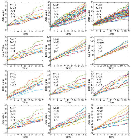
Figure 2.
Multi random effect gamma process degradation path.
These twelve sets of data sets have different model parameters, so as to compare the applicability of the method to different forms of data. In these twelve groups of data, 1 time unit is taken as a sample point, each data set contains degradation paths, and each degradation path contains data points. Data sets 1~3 have the same degenerate model parameters and the number of data points, but they contain different paths . Data sets 4~6 have the same degenerate model parameters and the number of paths, but they contain different data points . Data sets 7~9 have the same number of data points and paths, but their model parameters are different. Data sets 10 to 12 have the same number of data points and paths, but their model parameters are different.
It can be seen from Figure 2 that for different degradation model with different parameters, the degradation trajectory has different change trends. Among them, the parameter and represent the size and dispersion of the initial parameter value; the parameters and sum together determine the dispersion degree of the degradation path. When the parameter is fixed, the parameter and represent the dispersion degree of the degradation track; When the parameter and are fixed, the parameter represents the degradation rate of the parameter. Therefore, it can be seen that the multi-random effect gamma process has good applicability for different degradation paths.
4.2. Parameter Estimation Result
4.2.1. Estimation Results of Prior Parameters
Since initial parameters and can be estimated only by data initial values, this part focuses on the research of the estimation methods of gamma process parameters and . For different degraded data sets, the method established in Section 3.2 was used to pre-estimate the hyperparameters , and . The results are shown in Figure 3 and Figure 4.
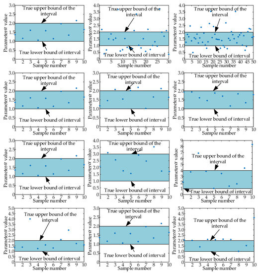
Figure 3.
Hyperparameter estimation results.
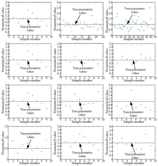
Figure 4.
Hyperparameter estimation results.
As can be seen from Figure 3, the hyperparameter is an interval value (), so for different data sets, most of the estimated value of hyperparameters fall into the real interval, but some of the estimates exceed the real parameter interval. When we choose a uniform distribution as the type of prior distribution of and , the distribution parameter can be assumed to be and , where and are the two smallest values of the hyperparameter , and are the two largest values of the hyperparameter . The estimated value of the hyperparameter distributed around the true value evenly. Therefore, uniform distribution is a reasonable prior distribution to model the hyperparameter . The distribution parameter can be assumed to be , where is the minimum estimated value of the hyperparameter and is the estimated maximum value of the hyperparameter .
To research the influence of prior distribution on parameter estimation results, different prior distribution types and parameters were used for unknown parameters. Where prior distribution 1 adopted gamma distribution for all unknown parameters , and ; Prior distribution 2 adopted uniform distribution for all unknown parameters; Prior distribution 3 adopted gamma distribution for parameter and , and uniform distribution for parameter . The results of parameter estimation are shown in Table 1 (it is noted that data sets 1, 4, 8 and 10 are the same, so the results of data sets 4, 8 and 10 are omitted in Table 1).

Table 1.
Parameter estimation result.
As shown in Table 1, when prior distribution 1 is adopted for unknown parameters, the estimated values have better estimated accuracy. It indicates that the gamma distribution can be used as prior distribution of unknown parameters and can obtain better estimated accuracy. When prior distribution 2 is adopted for the unknown parameters, the estimated accuracy of the parameters and is poor. Combined with Figure 3, when the moment method is used to estimate the hyperparameters, the randomness of the samples will cause some sample points to deviate from the boundary of the true interval, and the prior distribution of the parameters and is greatly affected by the boundary value of the hyperparameters estimated value. Combined with Figure 4, when the moment method is used to estimate the hyperparameter , the parameter estimated values of all samples are evenly distributed on both sides of the real value. When the uniform distribution is used as the prior distribution of the parameter , the accurate value of the prior distribution will lead to a more accurate posterior distribution after the likelihood function modification. On the whole, when prior distribution 3 is adopted for unknown parameters, it has good estimation accuracy for the unknown parameters. This is because prior distribution 3 combines the advantages of the above two prior distributions to achieve good estimation results for parameter , and .
4.2.2. Robustness Analysis of Parameter Estimation
The robustness of different prior distributions for degradation processes with different parameters was discussed in this part. Each degradation process in Figure 2 was simulated for 10 times, respectively, and the mean relative error (MRE) was used to calculate the statistical characteristics of parameter evaluation results under different prior distributions. The mean relative error of parameter estimation under different sample numbers is shown in Figure 5. It can be seen from Figure 5, with the increase in the sample number, the estimation errors of the prior distribution 1 and prior distribution 3 for the parameter and gradually decrease. This shows that the prior distribution without information can increase the accuracy of parameter estimation when the sample number is large. The estimation error of the prior distribution 2 for the parameter and increases with the increase in the sample number. The reason for this phenomenon is that extreme parameter estimation values is easy to produce by using the moment estimation method when the sample number is large. The uniform prior distribution constructed on this basis has a large error. With the increase in the sample number, the estimation accuracy of parameter with different prior distributions is improved.

Figure 5.
The MRE of different prior distributions under different sample numbers.
The mean relative error of parameter estimation under different sample point numbers is shown in Figure 6. On the whole, the accuracy of parameter estimation using different prior distributions will increase with the increase in the sample point number. Therefore, increasing the number of detection points in the degradation test can improve the accuracy of reliability assessment. There is a smaller parameter estimation error using the prior distribution 3.

Figure 6.
The MRE of different prior distributions under different sample point numbers.
The mean relative error of parameter estimation under different value is shown in Figure 7. The estimation error for using the prior distribution 2 is minimal, but the prior distribution 2 is unstable for the estimation of . On the whole, the prior distribution 3 has good stability for estimation of different parameters.

Figure 7.
The MRE of different prior distributions under different β value.
The mean relative error of parameter estimation under different value is shown in Figure 8. When the value is low, the dispersion of the degenerate trajectory is small, and the estimation error of the parameter is minimal. On the contrary, when the value is large, the dispersion of the degenerate trajectory is large, and the estimation error of the parameter is minimal.
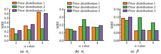
Figure 8.
The MRE of different prior distributions under different α value.
4.3. Lifetime Distribution Acquisition
The lifetime of samples can be obtained by the method established in Section 3.3, and the distribution characteristics of lifetime can be obtained by statistical methods. In this section, the lifetime distribution of data set 1 was calculated.
According to the characteristic of the stochastic process, the discrete time interval does not affect the value of lifetime distribution. However, when the time interval is too large, it will cause a certain error in the result. At the same time, the amount of computation will rapidly increase with small time interval. The changes of lifetime average and calculation time with discrete time are shown in Figure 9. It can be seen from the Figure 9, with the decrease in discrete time interval, the average life gradually converges to a certain value. However, the computation time increases rapidly with the decrease in discrete time interval. Therefore, when using the method in Section 3.3 to calculate the lifetime distribution, appropriate discrete time intervals should be selected to obtain more accurate calculation results with less calculation time.
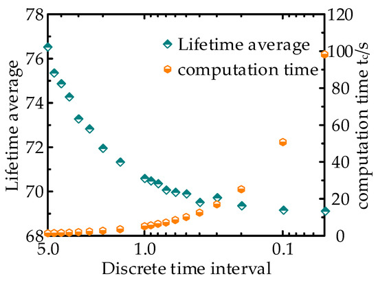
Figure 9.
Variation in lifetime mean and computation time with discrete time.
The changes in average lifetime and calculation time with the number of samples are shown in Figure 10. It can be seen from the Figure 10, when the number of samples is small, the average life has a large volatility. When the number of samples is greater than 1000, the volatility of the average life gradually decreases and gradually converges to a certain value. The calculation time will increase with the increase in the number of samples. Since the horizontal coordinate in the figure is a logarithmic coordinate system, the calculation time and the number of samples show an exponential change relationship. In fact, under the linear coordinate system, the calculation time will show a trend of linear increase with the increase in the number of samples.
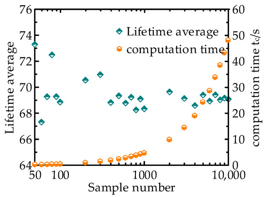
Figure 10.
Variation in lifetime mean and computation time with sample number.
The frequency histogram of lifetime values is shown in Figure 11. It can be seen from Figure 11, the lifetime value presents a positive skew distribution, that is, the curve is shorter on the left side and longer on the right side at the highest point. The statistical characteristics of the lifetime value are shown in Table 2. It can be seen from the Table 2 that the average value of the sample lifetime is greater than the median value, and the skewness of the sample lifetime is greater than 0, indicating a positive skewness distribution. The experience cumulative failure distribution obtained from the lifetime value of each sample is shown in Figure 12. According to the cumulative failure distribution, the lifetime value under any reliability can be obtained.
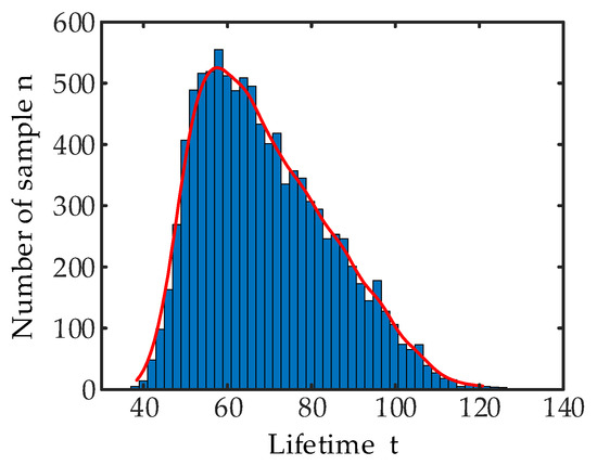
Figure 11.
Lifetime value frequency graph of data set 1.

Table 2.
Statistical characteristics of life value.
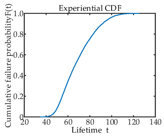
Figure 12.
Cumulative failure distribution of experience of data set 1.
5. Engineering Application
The wear degradation process of the aviation hydraulic rotary joint was analyzed in this Section. The fit clearance between the elbow joint and the nozzle sleeve is one of the main reasons that lead to the reliability reduction in the hydraulic rotary joint. When the fit clearance of the rotary joint increases to the specified failure threshold, the rotary joint is considered to have failed. The wear of the rotary joint is shown in Figure 13.
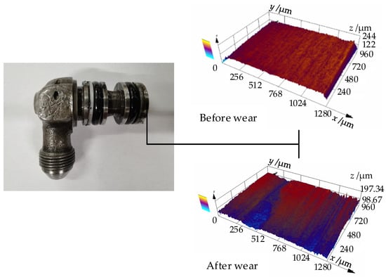
Figure 13.
Rotary joint wear diagram.
The variation in the fit clearance value with the number of reciprocating rotations is shown in Figure 14. It can be seen from Figure 14, the fit clearance of the hydraulic rotary joint shows a gradual increasing trend with the increase in the number of rotation. However, due to the randomness of wear and the measurement error, the variation in fit clearance of the same hydraulic rotary joint shows a certain random fluctuation, and the degradation trajectory of different hydraulic rotary joints is different, which is mainly manifested in the initial value and degradation rate are different. In this paper, the multi-random effect gamma random process is used to model the wear and degradation process of aviation hydraulic rotary joint, and based on this, the life of aviation hydraulic rotary joint was analyzed.
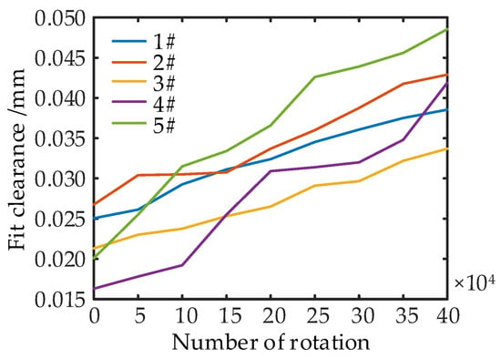
Figure 14.
Variation in fitting clearance with the number of reciprocating rotations.
The distribution test of wear increment was carried out using K-S test method, and the test result is shown in Table 3. The p-value of the test is 0.9163, which indicates that the wear degradation increment conforms to the gamma distribution. So, it is reasonable to use gamma process to analyze the wear degradation process of hydraulic rotary joint.

Table 3.
Wear increment distribution test.
Firstly, the data in Figure 14 were used to estimate the model parameters of the multi-random effect gamma process. It is assumed that the prior distribution of the parameter was gamma distribution , the prior distribution of the parameter was gamma distribution , the prior distribution of the parameter was gamma distribution , the prior distribution of the parameter was gamma distribution and the prior distribution obtained by the moment estimation method was uniform distribution . The parameter estimation results of the multi-random effect gamma process model extracted from Markov chain by MCMC-Gibbs sampling are shown in Table 4.

Table 4.
Parameter estimation results for multiple random effects gamma processes.
The threshold was set to 0.07 mm, the sample size was set to 1000, and the discrete time step was to 0.001. Figure 15 shows the frequency histogram of the life value of the aviation hydraulic rotary joint, and Table 5 shows the statistical characteristics of the life value. It can be seen from the Figure 11, the life value distribution has a strong skewness distribution, with a skewness of 1.3492. The life value has a large quantity distribution in the range of 500,000 times to 900,000 times.
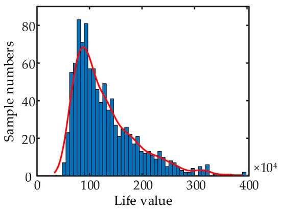
Figure 15.
Lifetime value frequency graph of hydraulic rotary joint.

Table 5.
Statistical characteristics of life value of hydraulic rotary joint.
The experience CDF obtained from the lifetime of each sample is shown in Figure 16. It can be seen that when the lifetime value is less than 1 million times, the cumulative failure probability of the aviation hydraulic rotary joint increases faster. According to the cumulative failure probability, the life value under any reliability can be obtained, which can provide reference for the replacement and maintenance of aviation hydraulic rotary joint.
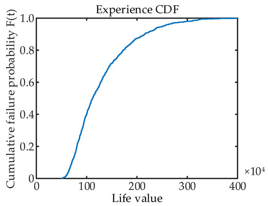
Figure 16.
Cumulative distribution of experience.
6. Conclusions
This study has proposed a reliability evaluation framework for gamma random degradation process with multiple random effects. The gamma process with multiple random effects established in this paper can well describe the product performance degradation process with monotonic and dispersive characteristics. Because prior distribution has an important influence on parameter estimation in Bayesian approach, this paper has discussed the construction method of prior distribution of unknown parameters.
The moment method has used to obtain the initial values of the degradation model parameters of different samples, and then the parameter values of the prior distribution have obtained. When gamma distribution was selected as the prior distribution of parameter and , uniform distribution was selected as the prior distribution of parameter , the accuracy of parameter estimates is the highest. The numerical experiments show that the proposed method can obtain good parameter estimation results.
The Monte Carlo method has used to obtain the sample life value, and the product reliability has obtained on this basis. It is found that the discrete time and the number of samples in the Monte Carlo method have a great impact on the calculation time. In order to maintain a balance between the calculation time and the calculation accuracy, it is necessary to select the appropriate discrete time and the number of samples. Statistics of the sample life value show that the average life value is greater than the median value, and the skewness of the sample life value is greater than 0, which conforms to the normal skewness distribution characteristics.
Author Contributions
Conceptualization, Z.Z. and D.G.; theoretical methodology, Z.Z. and T.G.; programming algorithms, Y.L. and J.Z.; calculation result analysis, Z.Z.; writing—original draft preparation, Z.Z., D.G., J.T. and Y.L.; writing—review and editing, D.G. and L.W.; supervision, D.G.; project administration, D.G. and L.W.; funding acquisition, D.G. and Y.L. All authors have read and agreed to the published version of the manuscript.
Funding
This work was supported by the Joint Foundation of National Natural Science Foundation of China [grant number U2233212]; the National Natural Science Foundation of China [grant number 52005428]; and the Natural Science Foundation of Hebei Province [grant number E2021203099].
Data Availability Statement
All e generated or analyzed during this study are included in this article.
Conflicts of Interest
The authors declare no conflict of interest.
References
- Yan, T.; Lei, Y.; Li, N.; Wang, B.; Wang, W. Degradation Modeling and Remaining Useful Life Prediction for Dependent Competing Failure Processes. Reliab. Eng. Syst. Saf. 2021, 212, 107638. [Google Scholar] [CrossRef]
- Liu, K.; Shang, Y.; Ouyang, Q. A Data-Driven Approach with Uncertainty Quantification for Predicting Future Capacities and Remaining Useful Life of Lithium-Ion Battery. IEEE Trans. Ind. Electron. 2021, 68, 3170–3180. [Google Scholar] [CrossRef]
- Zhang, J.; Hu, C.; He, X.; Si, X. A Novel Lifetime Estimation Method for Two-Phase Degrading Systems. IEEE Trans. Reliab. 2019, 68, 689–709. [Google Scholar] [CrossRef]
- Yang, N.; Wang, Z.; Cai, W.; Li, Y. Data Regeneration Based on Multiple Degradation Processes for Remaining Useful Life Estimation. Reliab. Eng. Syst. Saf. 2023, 229, 108867. [Google Scholar] [CrossRef]
- Zheng, H.; Yang, J.; Xu, H.; Zhao, Y. Reliability Acceptance Sampling Plan for Degraded Products Subject to Wiener Process with Unit Heterogeneity. Reliab. Eng. Syst. Saf. 2023, 229, 108877. [Google Scholar] [CrossRef]
- Taylor, P.; Lu, C.J.; Meeker, W.O. Using Degradation Measures to Estimate a Time-to- Failure Distribution Using Degradation Measures to Estimate a Time-to-Failure Distribution. Technometrics 2012, 35, 37–41. [Google Scholar]
- Wang, Z.; Hu, C.; Wang, W.; Si, X. An Additive Wiener Process-Based Prognostic Model for Hybrid Deteriorating Systems. IEEE Trans. Reliab. 2014, 63, 208–222. [Google Scholar] [CrossRef]
- Yan, B.; Ma, X.; Huang, G.; Zhao, Y. Two-Stage Physics-Based Wiener Process Models for Online RUL Prediction in Field Vibration Data. Mech. Syst. Signal Process. 2021, 152, 107378. [Google Scholar] [CrossRef]
- Li, Y.; Huang, X.; Ding, P.; Zhao, C. Wiener-Based Remaining Useful Life Prediction of Rolling Bearings Using Improved Kalman Filtering and Adaptive Modification. Meas. J. Int. Meas. Confed. 2021, 182, 109706. [Google Scholar] [CrossRef]
- Liu, D.; Wang, S.; Zhang, C. Reliability Estimation from Two Types of Accelerated Testing Data Based on an Artificial Neural Network Supported Wiener Process. Appl. Math. Comput. 2022, 417, 126757. [Google Scholar] [CrossRef]
- Wu, D.; Jia, M.; Cao, Y.; Ding, P.; Zhao, X. Remaining Useful Life Estimation Based on a Nonlinear Wiener Process Model with CSN Random Effects. Measurement 2022, 205, 112232. [Google Scholar] [CrossRef]
- Liu, D.; Duan, X.; Wang, S.; Cui, X.; Wu, X.; Niu, Y. A Reliability Estimation Method Based on Signal Feature Extraction and Artificial Neural Network Supported Wiener Process with Random Effects. Appl. Soft Comput. 2023, 136, 110044. [Google Scholar] [CrossRef]
- Liu, X.; Wu, Z.; Cui, D.; Guo, B.; Zhang, L. A Modeling Method of Stochastic Parameters’ Inverse Gauss Process Considering Measurement Error under Accelerated Degradation Test. Math. Probl. Eng. 2019, 2019, 9752920. [Google Scholar] [CrossRef]
- Ma, Z.; Liao, H.; Ji, H.; Wang, S.; Yin, F.; Nie, S. Optimal Design of Hybrid Accelerated Test Based on the Inverse Gaussian Process Model. Reliab. Eng. Syst. Saf. 2021, 210, 107509. [Google Scholar] [CrossRef]
- Fang, G.; Pan, R.; Wang, Y. Inverse Gaussian Processes with Correlated Random Effects for Multivariate Degradation Modeling. Eur. J. Oper. Res. 2022, 300, 1177–1193. [Google Scholar] [CrossRef]
- Duan, F.; Wang, G. Computers & Industrial Engineering Planning of Step-Stress Accelerated Degradation Test Based on Non-Stationary Gamma Process with Random effects. Comput. Ind. Eng. 2018, 125, 467–479. [Google Scholar] [CrossRef]
- Mercier, S.; Castro, I.T. Stochastic comparisons of imperfect maintenance models for a gamma deteriorating system. Eur. J. Oper. Res. 2018, 273, 237–248. [Google Scholar] [CrossRef]
- Ling, M.H.; Ng, H.K.T.; Tsui, K.L. Bayesian and Likelihood Inferences on Remaining Useful Life in Two-Phase Degradation Models under Gamma Process. Reliab. Eng. Syst. Saf. 2019, 184, 77–85. [Google Scholar] [CrossRef]
- Cholette, M.E.; Yu, H.; Borghesani, P.; Ma, L.; Kent, G. Degradation Modeling and Condition-Based Maintenance of Boiler Heat Exchangers Using Gamma Processes. Reliab. Eng. Syst. Saf. 2019, 183, 184–196. [Google Scholar] [CrossRef]
- Hua, P.; Xing, B.; Tao, F. Inference for Constant-Stress Accelerated Degradation Test Based on Gamma Process. Appl. Math. Model. 2019, 67, 123–134. [Google Scholar] [CrossRef]
- Paroissin, C. Online Estimation Methods for the Gamma Degradation Process. IEEE Trans. Reliab. 2017, 66, 1361–1367. [Google Scholar] [CrossRef]
- Song, K.; Shi, J.; Yi, X. A Time-Discrete and Zero-Adjusted Gamma Process Model with Application to Degradation Analysis. Physica A 2020, 560, 125180. [Google Scholar] [CrossRef]
- Fan, J.; Chen, Y.; Jing, Z.; Seid, M.; Cai, M. A Gamma Process-Based Degradation Testing of Silicone Encapsulant Used in LED Packaging. Polym. Test. 2021, 96, 107090. [Google Scholar] [CrossRef]
- Haowei, W.; Tingxue, X. Lifetime Prediction Based on Gamma Processes from Accelerated Degradation Data. Chin. J. Aeronaut. 2015, 28, 172–179. [Google Scholar] [CrossRef]
- Lin, C.P.; Ling, M.H.; Cabrera, J.; Yang, F.; Yu, D.Y.W.; Tsui, K.L. Prognostics for Lithium-Ion Batteries Using a Two-Phase Gamma Degradation Process Model. Reliab. Eng. Syst. Saf. 2021, 214, 107797. [Google Scholar] [CrossRef]
- Wang, H.; Liao, H.; Ma, X.; Bao, R. Remaining Useful Life Prediction and Optimal Maintenance Time Determination for a Single Unit Using Isotonic Regression and Gamma Process Model. Reliab. Eng. Syst. Saf. 2021, 210, 107504. [Google Scholar] [CrossRef]
- Belhaj, M.; Fouladirad, M.; Deloux, E. Variance Gamma Process as Degradation Model for Prognosis and Imperfect Maintenance of Centrifugal Pumps. Reliab. Eng. Syst. Saf. 2022, 223, 108417. [Google Scholar] [CrossRef]
- Wang, X.; Xing, B.; Hong, Y.; Hua, P. Degradation Data Analysis Based on Gamma Process with Random Effects. Eur. J. Oper. Res. 2021, 292, 1200–1208. [Google Scholar] [CrossRef]
- Rodríguez-picón, L.A.; Rodríguez-picón, A.P.; Carlos, L.; Rodríguez-borbón, M.I.; Alvarado-iniesta, A. Degradation Modeling Based on Gamma Process Models with Random Effects. Commun. Stat.-Simul. Comput. 2018, 47, 1796–1810. [Google Scholar] [CrossRef]
- Song, K.; Cui, L. A Common Random Effect Induced Bivariate Gamma Degradation Process with Application to Remaining Useful Life Prediction. Reliab. Eng. Syst. Saf. 2022, 219, 108200. [Google Scholar] [CrossRef]
- Tsai, C.; Tseng, S.; Balakrishnan, N. Optimal Design for Degradation Tests Based on Gamma Processes with Random Effects. IEEE Trans. Reliab. 2012, 61, 604–613. [Google Scholar] [CrossRef]
- Zhou, S.; Xu, A.; Tang, Y.; Shen, L. Fast Bayesian Inference of Reparameterized Gamma. IEEE Trans. Reliab. 2023. [Google Scholar] [CrossRef]
- Zhuang, L.; Xu, A.; Wang, X. A Prognostic Driven Predictive Maintenance Framework Based on Bayesian Deep Learning. Reliab. Eng. Syst. Saf. 2023, 234, 109181. [Google Scholar] [CrossRef]
Disclaimer/Publisher’s Note: The statements, opinions and data contained in all publications are solely those of the individual author(s) and contributor(s) and not of MDPI and/or the editor(s). MDPI and/or the editor(s) disclaim responsibility for any injury to people or property resulting from any ideas, methods, instructions or products referred to in the content. |
© 2023 by the authors. Licensee MDPI, Basel, Switzerland. This article is an open access article distributed under the terms and conditions of the Creative Commons Attribution (CC BY) license (https://creativecommons.org/licenses/by/4.0/).