A Customized IMOEA/D for Bi-Objective Single-Machine Scheduling with Adaptive Preventive Maintenance

Abstract

The prolonged operation of machines in the production process can lead to continuous deterioration or even failure, and the necessary maintenance measures can alleviate the above negative effects. For this reason, this study investigates a joint optimization problem of single-machine production and preventive maintenance (PM) considering linear deterioration effects. The objective is to obtain an integrated sequence of degrading jobs and PM activities in order to simultaneously minimize the makespan and the total cost. Based on the problem characteristics, an adaptive PM strategy is first designed. To efficiently solve the problem, an improved multi-objective evolutionary algorithm based on decomposition (IMOEA/D) is tailored, where the biased-distribution weight vector is proposed to enhance the search capability at both ends of the Pareto front. Five instances are used to evaluate the performance of the customized IMOEA/D and two classical multi-objective evolutionary algorithms. Numerical studies show that the IMOEA/D can substantially improve the hypervolume metric, the maximum spread metric, and the distributivity of the Pareto front at a slight sacrifice of the spacing metric.

1. Introduction

Single-machine scheduling usually refers to the scheduling of a set of production tasks on a single machine to optimize production metrics such as maximum completion time and total operation cost in a discrete manufacturing environment. Depending on the specific constraints and objectives, single-machine scheduling can be subdivided into different combinational optimization problems such as single-machine scheduling with the learning effect and deterioration effect [1], and single-machine scheduling considering time-and-resource-dependent processing times [2]. Some studies such as Martinelli et al. [3] have conducted a systematic survey of single-machine scheduling. From the above review, it can be seen that common approaches to solving single-machine scheduling include efficient polynomial-time algorithms [4,5,6], heuristics and metaheuristics [7,8,9].

A classic variant of single-machine scheduling is to consider machine unavailability during production scheduling [10,11,12]. Both machine breakdowns and preventive maintenance (PM) activities lead to temporary machine unavailability, the former resulting in forced downtime for repairs, while the latter is known in advance. This means that unexpected failures may interrupt jobs being processed, and there is no time overlap between PM planning and production scheduling. Another advantage of PM is that it improves the running condition of the machine, thus reducing the probability of unexpected failures [13,14,15]. The relevant literature has also demonstrated that PM plays an indispensable role in smart manufacturing for Industry 4.0 [16,17,18]. However, there is a major challenge to develop an appropriate maintenance strategy to balance the coupling conflicts between production and maintenance under a specific manufacturing scenario. For this reason, many researchers have been working on the integrated optimization of production scheduling and PM under different constraints and optimization requirements of single-machine manufacturing scenarios in the last two decades.

For example, Liao and Chen [19] assumed that each PM is required after a fixed interval on a single machine and employed the branch-and-bound algorithm and the heuristic, respectively, to solve small-sized and large-sized problems to minimize the maximum tardiness. Jin et al. [20] extended a multi-objective version of the integrated optimization of PM planning and single-machine scheduling proposed by Cassady and Kutanoglu [21] and presented a multi-objective genetic algorithm to simultaneously optimize five objectives. Low et al. [22] proved the studied single-machine scheduling problems with periodic and flexible PM are NP-hard and provided an efficient heuristic to obtain the minimal makespan. Luo et al. [5] considered a variable maintenance duration that increases with the starting time of PM and developed polynomial-time algorithms to deal, respectively, with four problem scenarios with different optimization objectives. Shen and Zhu [23] investigated an integrated scheduling problem of single-machine production and periodic maintenance targeted at minimizing the makespan, where uncertain processing time and maintenance duration were considered. Wang et al. [24] proposed a novel flexible PM mechanism that combines a time-based PM with a condition-based PM, and designed a Q-learning-based solution framework to tackle a single-machine scheduling problem considering the proposed flexible PM.

A review of relevant studies shows that joint optimization problems of single-machine scheduling and PM are more oriented towards single-objective optimization. Practical decision makers usually focus on multiple conflicting optimization objectives, which can be confirmed in other variants of single-machine scheduling. Choobineh et al. [25] considered sequence-dependent setup times and proposed a multi-objective tabu search algorithm to minimize the makespan, number of tardy jobs and total tardiness. Tavakkoli-Moghaddam et al. [26] built a fuzzy multi-objective linear programming model with the objective of minimizing the makespan and total weighted tardiness. Che et al. [27] introduced the power-down mechanism in single-machine scheduling and developed an advanced $\epsilon$-constraint method with local search to minimize the total energy consumption and maximum tardiness simultaneously. Similarly, Wu et al. [28] used $\epsilon$-constraint-based heuristic algorithms to solve a single-machine scheduling problem considering time-of-use electricity tariffs in order to optimize the makespan and total electricity cost. Compared to the above multi-objective single-machine scheduling problems, the studied integrated optimization problem requires joint decision making between the production and maintenance departments, thus it is more necessary to carry out a multi-objective optimization study for the optimization needs of the two departments.

This study addresses an integrated optimization problem of single-machine scheduling and PM with the objectives of minimizing the maximum completion time and the total cost of production and maintenance processes. Both the deterioration effects and stochastic failures are considered in the proposed integrated optimization problem. To improve these two negative effects as well as to adapt the characteristics of the studied bi-objective optimization, a novel adaptive PM strategy is designed for the trade-off between the maintenance time and maintenance cost. In addition, this study also introduces the minimal repair (MR) strategy to cope with unexpected failures. For efficiently solving the above problem, an improved multi-objective evolutionary algorithm based on decomposition (IMOEA/D) is tailored. The main contributions of the developed algorithm are reflected in the design of the decoding process and the improvement of the weight vector distribution.

The remainder of the study is organized as follows. In Section 2, the studied problem is systematically described and a novel PM strategy is proposed. Section 3 introduces the IMOEA/D that is used to solve the problem, followed by a series of numerical studies in Section 4 to evaluate the performance of the tailored IMOEA/D. Finally, some conclusions and future research directions are summarized in Section 5.

2. Single-Machine Scheduling with Adaptive PM

2.1. Problem Statement and Assumptions

There are $n$ jobs waiting to be processed on a single machine, and the machine’s age increases as the production process proceeds. The increase in the machine’s age will result in longer processing times for jobs and increases the probability of machine failures. As a consequence, machine maintenance activities are essential. In case of an unexpected machine breakdown, an MR will be carried out to restore the running condition of the machine without changing the machine’s age. To improve the machine’s age and reduce the probability of failures, PM is usually integrated into the single-machine scheduling.

The timing of PM intervention is one of the main focuses of the research on the integrated optimization problem. Excessive frequency of PM may result in over-maintenance, costing maintenance as well as loss of production profit due to taking up potential production time, while too long a period of time without PM can exacerbate the deteriorating condition of the machine as well as the probability of malfunctioning, which will result in a greater loss of unplanned downtime.

Different processing sequences have different impacts on machine deterioration, which also can influence the makespan. In addition, each job has a due date, and early delivery may lead to increased storage pressure in the shop floor, while late delivery may affect customer satisfaction. For this reason, in addition to the maintenance cost, the penalty cost of early and late delivery is considered in the total cost. The aim of the studied integrated optimization problem is to simultaneously minimize the makespan and the total cost. In addition, some problem assumptions are listed below.

(1)

All jobs can be processed by the machine at time 0 [29].

(2)

The processing of any job is not interrupted by proactive PM.

(3)

There are no additional constraints on the sequence of operations of the jobs.

(4)

The machine can only process one job at a time.

(5)

The processing time of a job increases linearly with the machine’s age, i.e., the deteriorating processing time as defined in Wang et al. [24].

(6)

The initial machine’s age is 0.

(7)

PM is performed to restore the machine’s age to 0.

(8)

MR will be carried out immediately after failures, to restore the running condition of the machine with the machine’s age unchanged.

2.2. Adaptive PM Strategy

Considering the objective optimization in both time and cost dimensions, this paper proposes an adaptive PM strategy for balancing maintenance time and maintenance cost. In terms of maintenance time, the probability of machine failure increases as the machine runs, the number of MRs increases, and the time taken for MRs may be greater than the time taken for PM, which means that PM carried out at the proper moment can save more maintenance time and greatly improve the machine’s age. The PM strategy based on maintenance time is concretely derived as follows.

First, we assume that the probability of machine failures and the age of the machine follow a two-parameter Weibull distribution with $\theta$ as the scale parameter and $\beta$ as the shape parameter. $\theta$ reflects the average time of occurrence of random failures, while $\beta$ determines the trend of the failure probability. When $\beta >1$, the failure rate gradually increases with the machine’s age; when β = 1, the failure rate is constant; when β < 1, the machine has a high probability of failures at the initial stage, but the failure rate decreases gradually with the increase in the machine’s age. To fit the reality, β > 1 is taken in the proposed problem. The probability density function $f\left(a\right)$ and the corresponding cumulative distribution function $F\left(a\right)$ of the Weibull distribution are shown in Equations (1) and (2), respectively, where $a$ denotes the machine’s age.

$$f\left(a\right)=\frac{\beta }{\theta }{\left(\frac{a}{\theta }\right)}^{\beta -1}{e}^{-{\left(\frac{a}{\theta }\right)}^{\beta }}$$

(1)

$$F\left(a\right)={\int }_0^{a}f\left(a\right)da=1-e^{-{\left(\frac{a}{\theta }\right)}^{\beta }}$$

(2)

Hence, the mapping relationship between the machine’s age and the probability of failures is obtained, as shown in Figure 1. Once the machine’s age $a_j$ after the completion of the job at the $j\mathrm{th}$ position has been determined, the corresponding failure rate $F\left(a_j\right)$ can be derived.

Thus, the expectation $E\left(N_f\right)$ of the number of machine failures as the machine’s age varies from $a_1$ to $a_j$ can be expressed by the following Equation (3). Assuming that the times spent on PM and an MR are $T_P$ and $T_M$, respectively, the maintenance threshold $A_T$ based on the maintenance time decision can be calculated from Equation (4). Similarly, in terms of maintenance cost, supposing that the costs spent on PM and an MR are $C_P$ and $C_M$, respectively, the maintenance threshold $A_C$ based on the maintenance cost decision can be obtained based on Equation (5).

$$E\left(N_f\right)={\sum }_{m=1}^{j}F\left(a_m\right)$$

(3)

$$A_T=\mathit{min}\left\{a_j\left|T_M{\sum }_{m=1}^{j}F\left(a_m\right)>T_P\right.\right\}$$

(4)

$$A_C=\mathit{min}\left\{a_j\left|C_M{\sum }_{m=1}^{j}F\left(a_m\right)>C_P\right.\right\}$$

(5)

To balance the time-based and cost-based decisions, we calculate the mean value of $A_T$ and $A_C$ as the used maintenance threshold $A$ in the subsequent experiments. When a job is processed and the machine’s age exceeds $A$, PM will be performed to restore the machine’s age to 0. In addition, different processing sequences correspond to different values of $A$, i.e., different PM strategies, which is regarded as an adaptive PM strategy in this paper.

3. The Developed IMOEA/D

Compared to the traditional non-dominated sorting genetic algorithm (NSGA-II), the MOEA/D algorithm reduces the complexity of the problem by converting the multi-objective problem into a series of single-objective subproblems. The weight vectors are used to represent the importance of the subproblems, and the neighborhood search strategy is employed to perform an effective local search, so as to find the approximate Pareto optimal solutions in the solution space that satisfy the requirements of different weights. Considering the characteristics of the proposed discrete combinatorial optimization problem, this paper designs an efficient decoding strategy and proposes a biased-distribution weight vector, which are the main innovations in the developed IMOEA/D. Specific details will be given in the following subsections.

3.1. Encoding and Decoding

Simple integer coding can represent the scheduling sequence on a single machine, where each integer code represents a job. In the studied integrated optimization problem of single-machine scheduling and PM, in addition to the scheduling of production sequences, the evaluation of machine failures and the judgment of the start time of the MR and PM are required, which are determined in the following decoding process.

Each job is processed sequentially according to the order of the integer encoding. After each job is processed, the probability of machine failures can be calculated based on the machine’s age, and thus the expectation of machine failure time can be calculated from the duration of the processing time and the failure rate, and then the expectation number of equivalent MR can be obtained. In addition, based on the adaptive PM strategy in Section 2.2, the PM intervention time can be determined for the current integer encoding. The detailed decoding process is presented in Algorithm 1.

Algorithm 1 Decoding procedure of the studied problem
Input: Individual encoding $I$
Output: Integrated optimization sequence, makespan, and the total cost
1	Let cumulative time $T_{online}$ since startup be 0
2	Let the number $n_{PM}$ of PMs be 0
3	Let the expectation number $n_{MR}$ of equivalent MR be 0
4	Calculate the PM intervention threshold $A$ for $I$ based on Section 2.2
5	for job in $I$ do
6	Obtain the deteriorating processing time $\tilde{P}$ and update the machine’s age $a$
7	$T_{online}\leftarrow T_{online}+\tilde{P}$
8	if $a>A$ then
9	$n_{PM}\leftarrow n_{PM}+1$
10	$T_{online}\leftarrow T_{online}+T_P$
11	$a\leftarrow 0$
12	end if
13	Calculate the failure rate $P$ based on $a$
14	$n_{MR}\leftarrow n_{MR}+P$
15	$T_{online}\leftarrow T_{online}+T_M·P$
16	end for
17	Calculate the makespan and the total cost

3.2. Biased-Distribution Weight Vector

In the standard MOEA/D algorithm, the weight vectors are generated using a uniform distribution in order to realize that the solution space is uniformly searched. This approach is suitable for problems with uniformly distributed solutions and can effectively explore the solution space to obtain more uniformly distributed solutions. By using the standard NSGA-II algorithm to solve the proposed problem, it can be found that the distribution of solutions is higher in the middle section of the Pareto front and lower at the two ends. This also means that the uniformly distributed weight vectors in the standard MOEA/D algorithm cannot focus the search on the regions with less solution distribution. In order to increase the search effort on both ends of the Pareto frontiers, a biased-distribution weight vector is designed as follows.

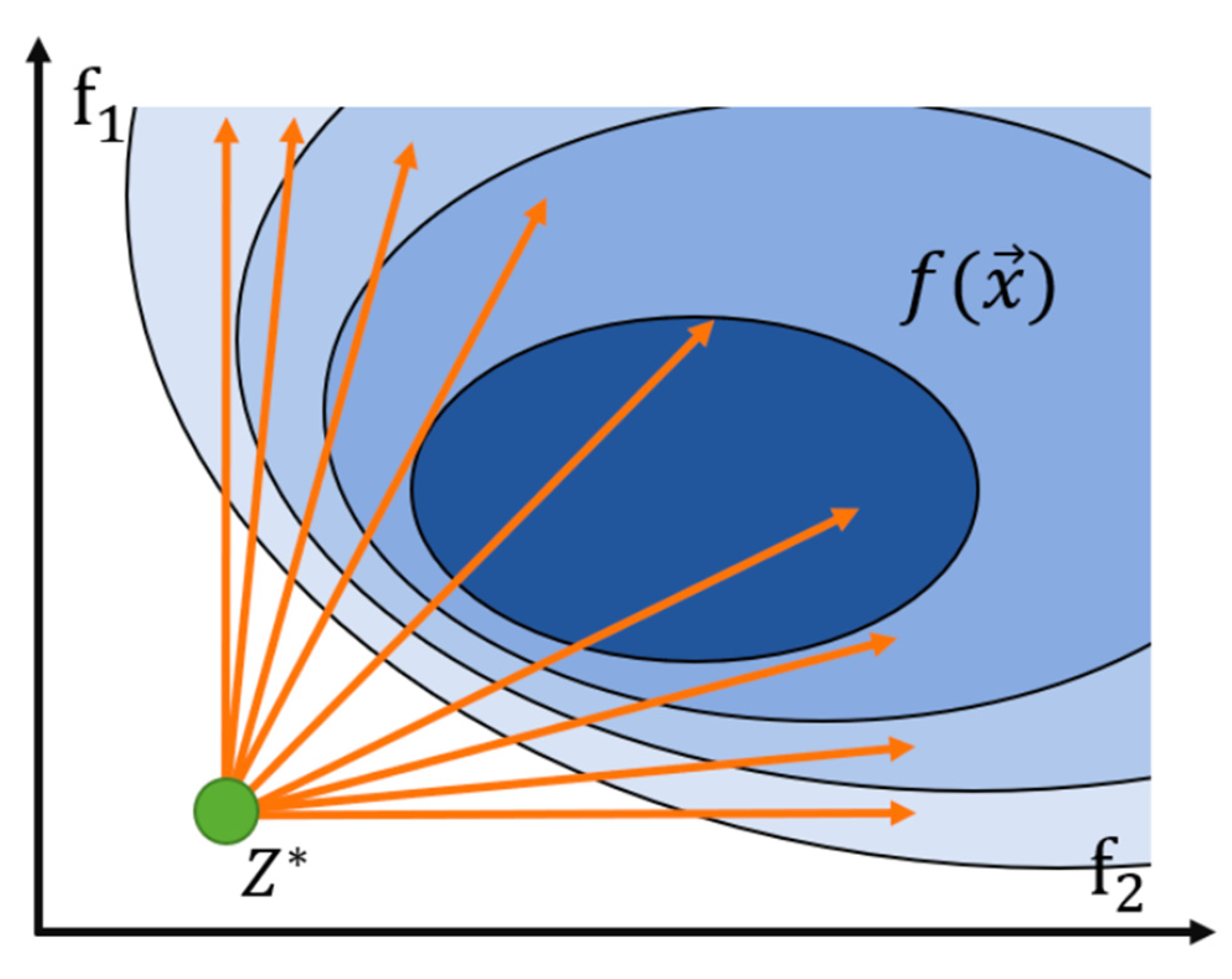
As shown in Figure 2, more dense weight vectors are configured at both ends of the Pareto frontiers with fewer distributions, while the configuration of weight vectors is appropriately reduced in the middle section of the Pareto frontiers with dense distributions, which improves the maximum spread metric and spacing metric of the Pareto frontiers, but may affect the number of solutions in the middle section of the Pareto frontiers to some extent. Z* is the reference point, where each objective is the minimum value of the corresponding objective set.

Let the set of uniformly distributed weight vectors $W$ be as Equation (6), where $x_i~U\left(\mathrm{0,1}\right)$ denotes that $x_i$ obeys a uniform distribution from 0 to 1, and $N$ denotes a total of $N$ weight vectors. Hence, the set of the biased-distribution weight vector $W^{\prime }$ can be defined by Equation (7), where $\phi \left(x_i\right)$ is a mapping function of $x_i$ in the uniformly distributed weight vector $\left(x_i,y_i\right)$ to $x_i^{\prime }$ in the biased-distribution weight vector $\left(x_i^{\prime },y_i^{\prime }\right)$. Regarding the settings of $\phi \left(x_i\right)$, we were inspired by the function curve in Figure 1 to define Equation (8), because this type of function can make the solutions of Equation (7) satisfy the characteristics of the biased-distribution weight vector (see Figure 3). We conducted extensive experiments and finally determined a better definition of $\phi \left(x_i\right)$ with scale parameter ${\theta }^{\prime }$ and shape parameter ${\beta }^{\prime }$ as 0.5 and 5.

$$W=\left\{\left(x_i,y_i\right)|x_i+y_i=1, x_i~U\left(\mathrm{0,1}\right), i=\mathrm{1,2},\cdots N\right\}$$

(6)

$$W^{\prime }=\left\{\left(x_i^{\prime },y_i^{\prime }\right)|x_i^{\prime }+y_i^{\prime }=1, x_i^{\prime }=\phi \left(x_i\right),x_i~U\left(\mathrm{0,1}\right), i=\mathrm{1,2},\cdots N\right\}$$

(7)

$$\phi \left(x_i\right)=1-e^{-{\left(\frac{x_i}{{\theta }^{\prime }}\right)}^{{\beta }^{\prime }}}$$

(8)

3.3. Overall Framework of the IMOEA/D

The detailed steps of the developed IMOEA/D are given below and the corresponding pseudo code is presented in Algorithm 2.

(1)

Initialize the population and then, respectively, calculate two optimization objectives of each individual, and then an initial reference point is determined based on the minimal makespan and minimal total cost among all the individuals.

(2)

Initialize the list of the biased-distribution weight vector based on Section 3.2. In addition, the number $\pi$ of neighbors is given.

(3)

Find the $\pi$ nearest neighbors for each individual in the population. Two of these neighbors are randomly selected for two-point crossover to generate new individuals, which is immediately followed by a mutation process that arbitrarily exchanges the two coding positions for the new individuals with a certain probability.

(4)

The individual with higher dominance is selected. If two new individuals do not dominate each other, one individual is randomly retained. Then, the reference point is updated.

(5)

Update the neighbors of each individual by comparing the Chebyshev distance between each neighbor and the reference point with the Chebyshev distance between the corresponding new individual and the reference point.

(6)

Update the non-dominated solution set based on the new individual.

(7)

If the number of iterations does not reach the set maximum number of iterations, go to step (3).

Algorithm 2 Pseudo code of the proposed IMOEA/D
Input: Maximum number $\mathsf{\Omega }$ of iterations
Output: Non-dominated solution set $\Gamma$, i.e., Pareto front
1	Initialize the population with $\mu$ individuals and the reference point $\varpi$
2	Initialize the biased-distribution weight vector and the number $\pi$ of neighbors
3	Let the non-dominated solution set $\Gamma =\left[\right]$
4	for iteration = 1: $\mathsf{\Omega }$ do
5	for individual = 1: $\mu$ do
6	Find the $\pi$ nearest neighbors for individual
7	Generate two new individuals based on crossover and mutation operators
8	Retain one new individual $I^{*}$ with higher dominance
9	Update the reference point $\varpi$
10	for neighbor = 1: $\pi$ do
11	Calculate the Chebyshev distance $d_1$ between neighbor and $\varpi$
12	Calculate the Chebyshev distance $d_2$ between $I^{*}$ and $\varpi$
13	if $d_2<d_1$ then
14	neighbor $\leftarrow I^{*}$
15	end if
16	end for
17	end for
18	if $\Gamma =\left[\right]$ then
19	Append $I^{*}$ in $\Gamma$
20	else
21	Compare $I^{*}$ with the solutions in $\Gamma$ and update $\Gamma$
22	end if
23	end for

4. Numerical Study

First, the workshop production data was initialized in this section, and immediately after that, three metrics including the HV metric, the spacing metric and the maximum spread metric were introduced for performance evaluation of the customized IMOEA/D. Finally, the superiority of the IMOEA/D was verified by comparing it with advanced multi-objective optimization algorithms under given instances. All algorithms were implemented in Python 3.8 and run on an Intel(R) Core(TM) i7-8700 CPU (3.20 GHz/16.00 GB RAM) PC.

4.1. Instance Settings

To evaluate the performance of the customized IMOEA/D, a total of five instances with different job numbers were set up. The job number was selected from {20, 30, 40, 50, 60}. Normal Processing time for each job followed a uniform distribution from 5 to 20. Deteriorating rate of each job was selected from {0.01, 0.02, 0.03, 0.04, 0.05}. Due date of each job was randomly generated from 50 to 600. For further visualization and comparative analysis, instance 2 with 30 deteriorating jobs is given in

Table 1. Basic parameter settings of jobs for instance 2.

Serial Number of Jobs	Normal Processing Time	Deteriorating Rate	Due Date
1	15	0.03	391
2	8	0.04	543
3	15	0.02	353
4	12	0.03	297
5	18	0.03	50
6	14	0.04	372
7	20	0.03	259
8	8	0.04	467
9	20	0.02	278
10	14	0.04	410
11	11	0.01	524
12	20	0.03	145
13	18	0.04	126
14	16	0.04	334
15	19	0.01	600
16	6	0.03	505
17	5	0.05	107
18	14	0.02	183
19	12	0.05	88
20	11	0.04	240
21	12	0.02	562
22	8	0.03	69
23	16	0.03	202
24	18	0.04	486
25	20	0.03	316
26	14	0.04	448
27	15	0.02	581
28	9	0.04	429
29	15	0.01	164
30	18	0.03	221

. In addition, penalty factors for early and late delivery of jobs were both 1. The two parameters $\theta$ and $\beta$ in the Weibull distribution used to characterize machine failures were set to 220 and 3, respectively. The time and cost consumed by an MR were set to 15, 200, and the time and cost consumed by PM were defined as 30, 600. Regarding the key parameters of IMOEA/D, the maximum iteration number and population number were set to 2000 and 200, and the number $\pi$ of neighbors was set to 5.

4.2. Performance Metric

4.2.1. HV Metric

In the two-dimensional target space formed by the two objective functions, the HV metric [30] represents the area of the target space dominated by the Pareto front. Before calculating the HV metric, a reference point needs to be selected. The location of this reference point needs to satisfy that the value of each objective function is greater than all the non-dominated solutions on the Pareto front. For convenience, solutions on the Pareto front are usually normalized and then the reference point can be set to (1.01, 1.01). A higher HV metric means that the algorithm performs better.

4.2.2. Spacing Metric

The spacing metric [31] is a measure of the homogeneity and continuity of the Pareto front. It is usually calculated as follows: Euclidean distances between every two neighboring solutions are calculated and the average of these distances is taken. The smaller the average distance is, the closer the Pareto front converges to a uniform and continuous distribution, i.e., the algorithm performs better when the spacing metric is smaller.

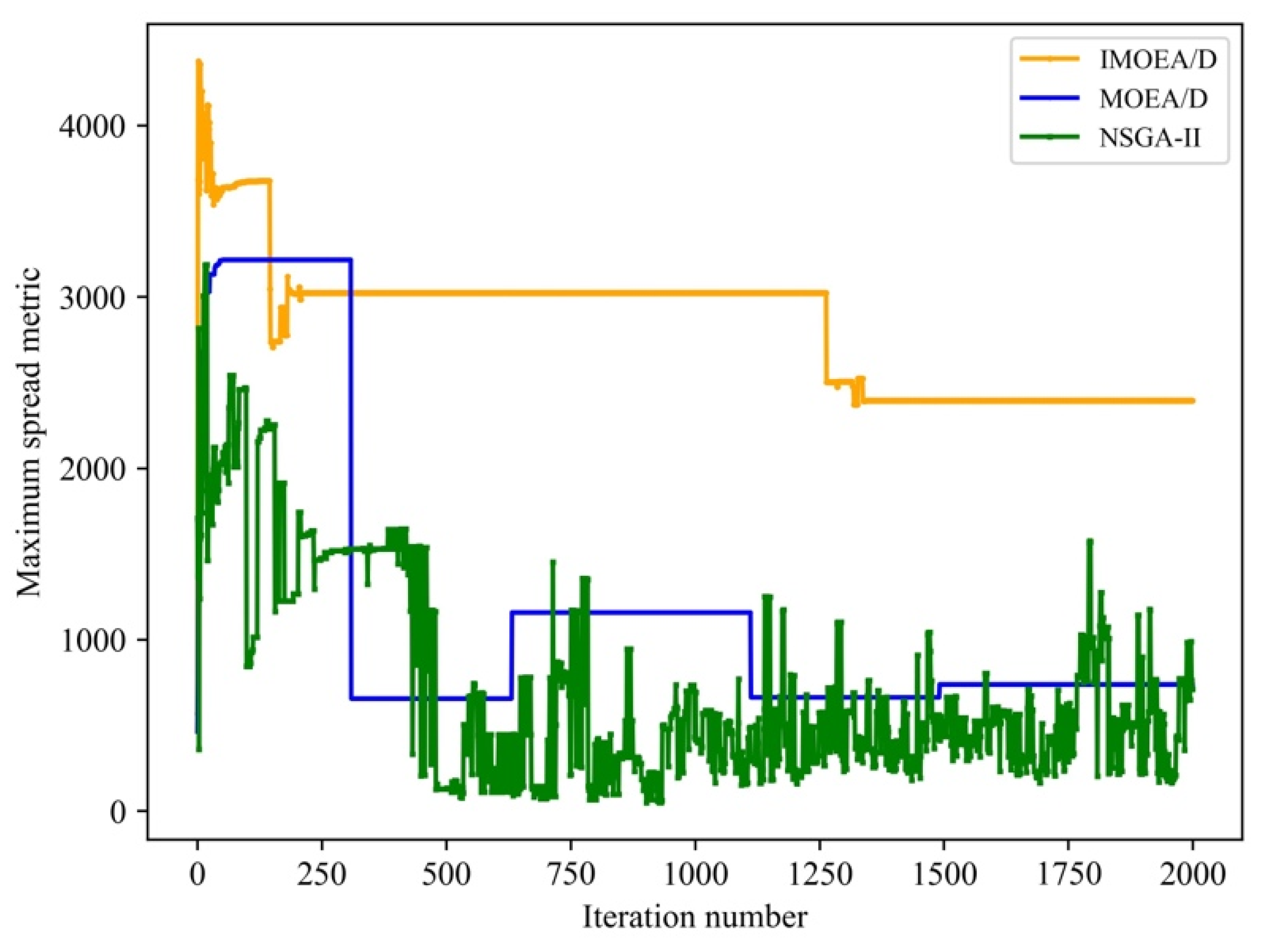
4.2.3. Maximum Spread Metric

The maximum spread metric [32] is the maximum value of the difference between the distances of all solutions to the leftmost and rightmost solutions on the Pareto front, which can reflect the distribution of the set of solutions in the domain of objective function values. The larger the maximum spread metric, the better the spread of solutions, i.e., the better the performance of the algorithm.

4.3. Performance Evaluation of IMOEA/D

To evaluate the solving performance of the developed IMOEA/D, two classical multi-objective optimization algorithms, including the standard MOEA/D and NSGA-II, were selected as algorithm rivals. It is noted that MOEA/D keeps the same configuration as IMOEA/D except for the biased-distribution weight vector. In addition, all the competing algorithms have the same population size and the same maximum iteration number that allows algorithms to converge. Each algorithm was run independently 10 times under each instance to achieve consistent and reliable results. As shown in

Table 2. Statistical results of HV metric of three algorithms in all instances.

Instance	Job Number	NSGA-II		MOEA/D		IMOEA/D
		Mean	Std	Mean	Std	Mean	Std
1	20	0.55	0.15	0.74	0.01	0.80	0.05
2	30	0.54	0.10	0.69	0.06	0.79	0.02
3	40	0.67	0.11	0.77	0.14	0.87	0.06
4	50	0.74	0.13	0.81	0.08	0.84	0.02
5	60	0.56	0.11	0.76	0.05	0.79	0.05

,

Table 3. Statistical results of spacing metric of three algorithms in all instances.

Instance	Job Number	NSGA-II		MOEA/D		IMOEA/D
		Mean	Std	Mean	Std	Mean	Std
1	20	12.52	14.49	3.61	1.24	2.44	0.42
2	30	24.22	29.23	25.27	18.71	10.23	2.61
3	40	77.28	75.80	5.35	3.89	23.25	23.35
4	50	85.40	58.17	6.86	3.41	10.17	3.46
5	60	90.86	112.28	13.72	10.36	12.31	3.77

and

Table 4. Statistical results of maximum spread metric of three algorithms in all instances.

Instance	Job Number	NSGA-II		MOEA/D		IMOEA/D
		Mean	Std	Mean	Std	Mean	Std
1	20	245.54	82.25	540.30	55.18	1030.96	357.99
2	30	467.72	293.31	916.04	235.24	3452.39	449.57
3	40	748.89	477.79	651.86	399.36	3181.33	329.57
4	50	333.06	254.67	613.52	167.89	2210.63	523.37
5	60	410.28	422.19	422.26	301.74	1257.38	359.27

, a detailed comparison of the mean and variance of the algorithm results is presented in terms of the HV metric, the spacing metric, and the maximum spread metric, respectively. It is observed that the developed IMOEA/D outperforms other algorithms in terms of the HV metric and the maximum spread metric, while it performs slightly worse than MOEA/D in terms of the spacing metric under instances 3 and 4. The reason for this is because an increase in the maximum spread metric may make the spacing of the points on the Pareto frontier subsequently increase, resulting in a slight sacrifice of the spacing metric. However, in terms of the HV metric, IMOEAD yields a better Pareto front.

To enhance the visualization of comparative results, we conducted further analysis for instance 2 from four perspectives: the Pareto front, the HV metric, the spacing metric, and the maximum spread metric. Some findings and conclusions are summarized as follows.

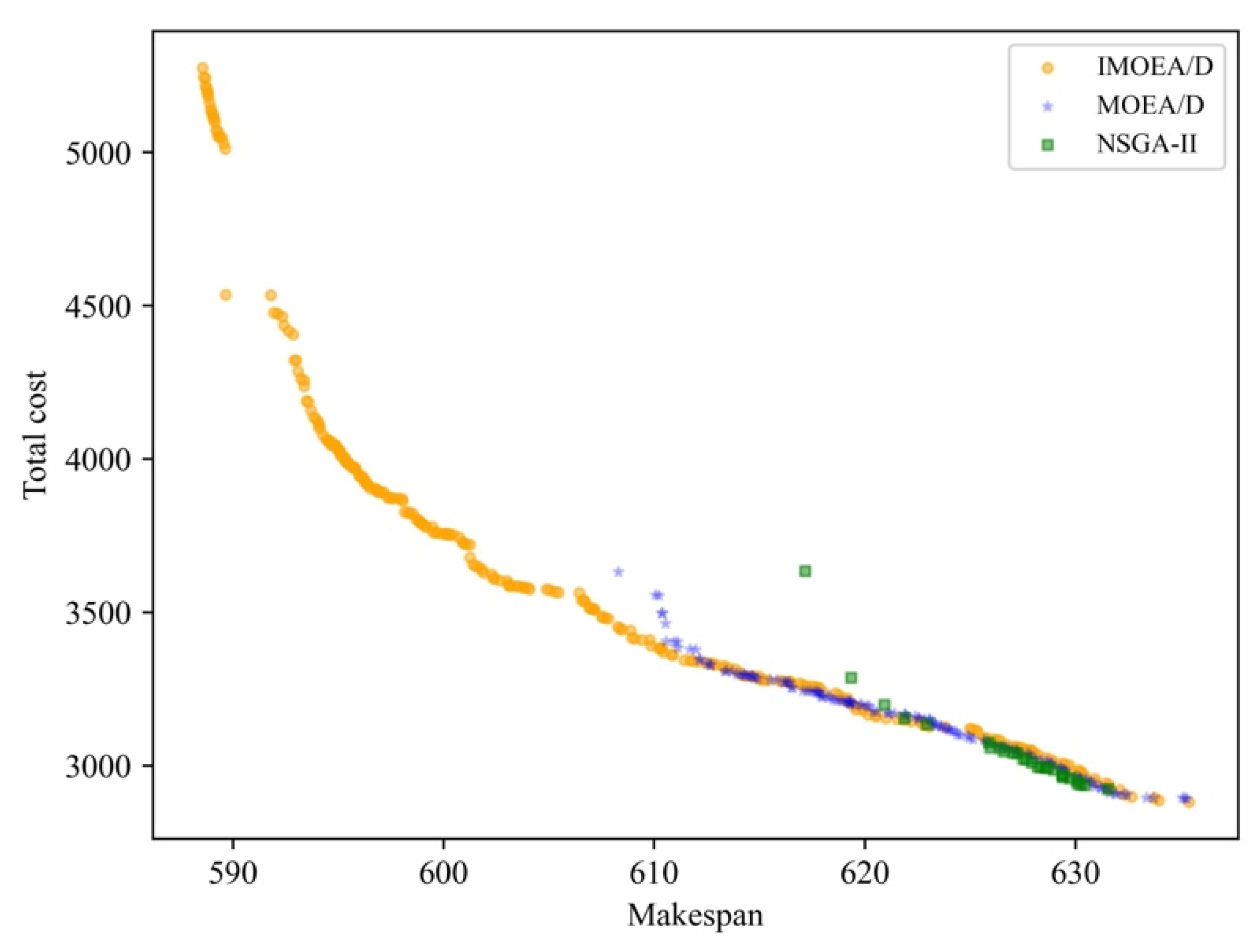
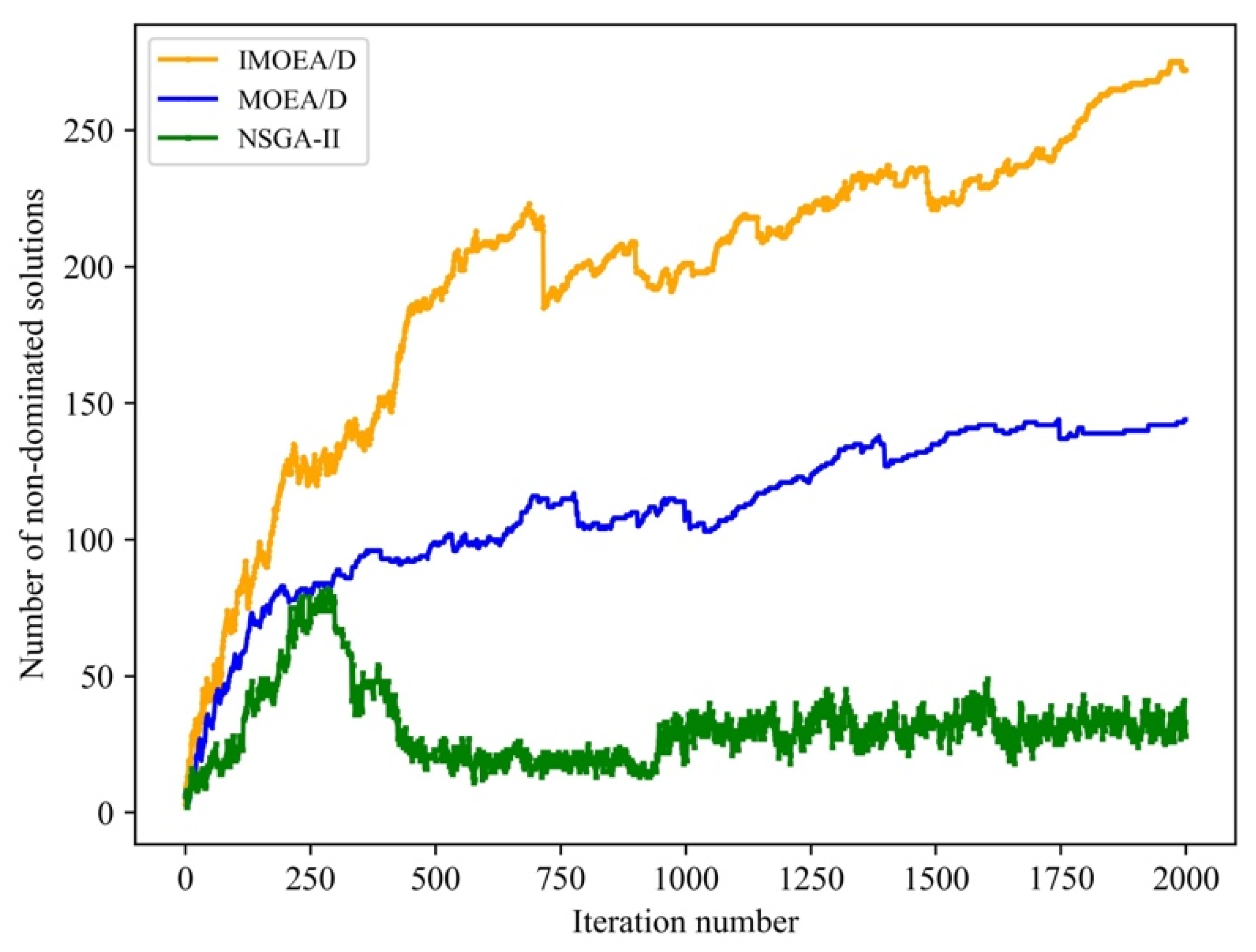
Firstly, the comparative result in terms of the Pareto front is shown in Figure 4. It can be intuitively seen that the distribution of the solutions of NSGA-Ⅱ is more concentrated compared to the two MOEA/D algorithms. This indicates that NSGA-Ⅱ has some limitations when dealing with the studied multi-objective optimization problem. Specifically, this is due to the relative inadequacy of NSGA-II in maintaining population diversity, resulting in its inability to efficiently search for non-dominated solutions in the entire solution space. In contrast, MOEA/D algorithms have better search performance in the target space by bootstrapping based on subproblems with the weight vector. IMOEA/D outperforms MOEA/D because MOEA/D uses the uniformly distributed weight vector, which may cause the algorithm to search insufficiently on both sides of the Pareto front to find more non-dominated solutions. This means that IMOEA/D can increase the search on both sides of the Pareto front to improve MOEA/D. The trend of the number of non-dominated solutions on Pareto front with increasing iteration number is shown in Figure 5. This also reflects the excellent performance of IMOEA/D in the search process.

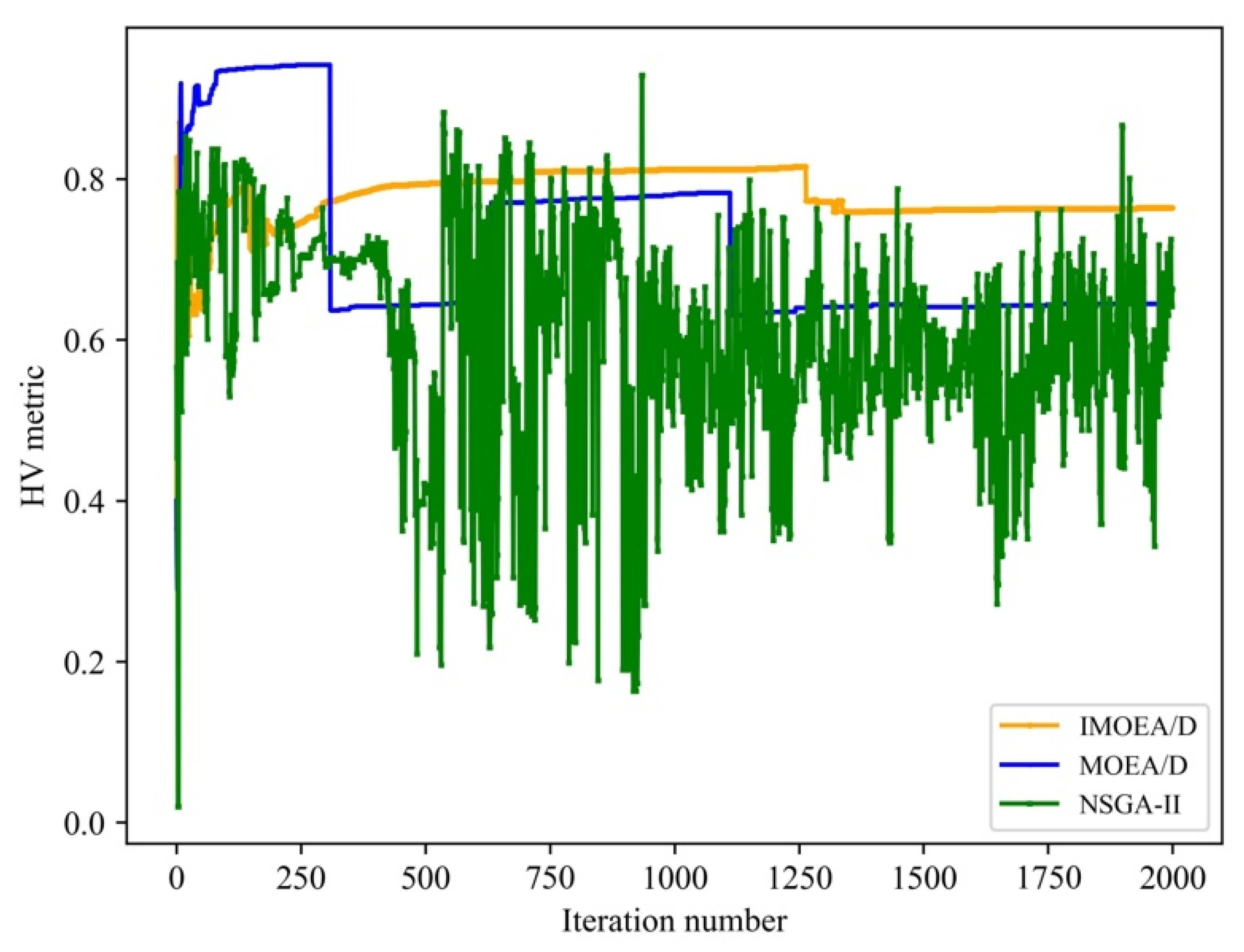
Secondly, the comparative result in terms of the HV metric is illustrated in Figure 6. The HV metric of IMOEA/D is the best, mainly due to the setting of the biased-distribution weight vector and the gain from IMOEA/D searching for more solutions on both sides of the Pareto front. This gain is mainly brought about by the preservation of population diversity during the iteration process. The HV metric of NSGA-II is comparable to that of MOEA/D, but some fluctuations are still present in the later iterations.

Next, the comparative result in terms of the spacing metric is given in Figure 7. The arrow points to the local magnification of the change of the spacing metric. It is clear that the spacing metric of the three algorithms converges quickly. The spacing metric of IMOEA/D is the best, followed by MOEA/D. The minimal spacing metric of NSGA-II is comparable to that of MOEA/D, while the convergence process of NSGA-II is not stable.

Finally, the comparative result in terms of the maximum spread metric is given in Figure 8. IMOEA/D has the best spread metric, followed by MOEA/D and NSGA-II. This is mainly due to the fact that IMOEA/D searches for more solutions at both ends of the Pareto front. Therefore, the distribution of solutions obtained by NSGA-II and MOEA/D-I is more centralized and less scalable, as can also be visualized in Figure 4.

5. Conclusions

This study proposed a customized IMOEA/D for solving a joint optimization of single-machine production scheduling and PM with the objectives of minimizing the makespan and total cost. The main contributions can be summarized as the following two aspects. On the one hand, an adaptive PM strategy was designed for the trade-off between the maintenance time and maintenance cost in order to improve the makespan and total cost to some extent. On the other hand, from the perspective of the algorithm design, an effective decoding strategy as well as the biased-distribution weight vector were introduced to improve the MOEA/D and adapt to the problem characteristics. Numerical studies shows that the developed IMOEA/D outperforms two other multi-objective optimization algorithms in terms of the Pareto front, HV metric and maximum spread metric, while the spacing metric of IMOEA/D is slightly worse than that of MOEA/D under some scenarios.

In future research, we will focus on the application of multi-objective integrated optimization of production scheduling and maintenance activities in more complex manufacturing scenarios. Firstly, more realistic constraints should be considered, such as human resources, spatial limitations and time-of-use tariffs. Secondly, more efficient multi-objective evolutionary algorithms need to be developed. The integration of the reinforcement learning algorithm and multi-objective evolutionary algorithms is a potential research trend. Thirdly, how to make decisions with respect to the non-dominated solutions obtained from the Pareto front is also an issue of great interest to decision makers.