Abstract
In recent years, industries have increasingly emphasized the need for high-speed, energy-efficient, and cost-effective solutions. As a result, there has been growing interest in developing flexible link manipulator robots to meet these requirements. However, reducing the weight of the manipulator leads to increased flexibility which, in turn, causes vibrations. This research paper introduces a novel approach for controlling the vibration and motion of a two-link flexible manipulator using reinforcement learning. The proposed system utilizes trust region policy optimization to train the manipulator’s end effector to reach a desired target position, while minimizing vibration and strain at the root of the link. To achieve the research objectives, a 3D model of the flexible-link manipulator is designed, and an optimal reward function is identified to guide the learning process. The results demonstrate that the proposed approach successfully suppresses vibration and strain when moving the end effector to the target position. Furthermore, the trained model is applied to a physical flexible manipulator for real-world control verification. However, it is observed that the performance of the trained model does not meet expectations, due to simulation-to-real challenges. These challenges may include unanticipated differences in dynamics, calibration issues, actuator limitations, or other factors that affect the performance and behavior of the system in the real world. Therefore, further investigations and improvements are recommended to bridge this gap and enhance the applicability of the proposed approach.
1. Introduction
Current industrial robots generally have their work-plan programmed or hardcoded, so that it is necessary to program the robot from scratch each time the production process changes. This process is time consuming and costly, requiring elaborate technical expertise [1,2]. In addition, conventional industrial robots have high rigidity so that sufficient positioning accuracy can be obtained but, in recent years, high speed and energy efficiency, as well as a reduction in cost for work, is required in the industries. This has led to increasing interest in the production of flexible link manipulator robots. There are several advantages stemming from the use of light-weight flexible-link manipulators, such as faster operation, lower energy consumption, and higher load-carrying capacity for the amount of energy expended [3,4]. Weight reduction is desirable; however, when the manipulator is made lighter, it becomes inevitably flexible, increasing vibration [5,6]. Therefore, it is necessary to consider the flexure and vibration due to the elasticity of the robot-arm.
Vibration and position control has been performed using varying strategies and methodologies, according to the literature. The authors of [7] developed a model-based controller for a flexible manipulator. PID and other hybrid strategies have been applied in [7,8,9]. Other strategies, like fuzzy logic, shape memory alloy (SMA), have also been utilized [7,10,11]. Conventional strategies for position and vibration control, such as PID control, model-based control, and frequency-based control, rely on mathematical models and predefined control algorithms. They require knowledge of system dynamics and parameter tuning. On the other hand, machine learning approaches learn control policies directly from data without explicitly modeling the system. Machine learning methods offer adaptability, the ability to handle complex systems, and do not require precise system models. However, the algorithms have higher implementation complexity, and may require extensive training. The choice between conventional strategies and machine learning models depends on the specific control problem, available system knowledge, and desired performance. In this paper, the focus is on the use of machine learning, specifically, reinforcement learning.
In recent years, reinforcement learning has been attracting attention in robotics and manufacturing industries [12,13,14]. Reinforcement learning (RL) is a type of machine learning capable of complex control schemes without the need for correct labels and large amounts of data. Consequently, RL has proven to be valuable in various applications in robotics. Researchers have explored the use of RL algorithms to enhance control, trajectory planning, grasping, and vibration control, amongst other in the robotics. Some studies in this field include the work by Xiaoming et al. [15], who investigated the optimal control problem of heavy material handling manipulators for agricultural robots with unknown robot parameters.
Xie et al. developed a sliding mode controller using a decoupling method to simultaneously control the angular movements of a three-rigid-link robotic manipulator and the attitude and position of an 8U CubeSat [16]. Zhi-cheng et al. devised a hybrid control strategy combining motion trajectory optimization and piezoelectric active control for a flexible hinged plate [17]. They utilized finite element modeling and experimental system identification to obtain accurate models of the piezoelectric driving and motor acceleration driving of the joint, and trained modal active controllers using an auto-soft-actor-critic RL algorithm.
Authors in [11] tackled the continuous-time optimal tracking control problem of an SMA actuated manipulator with prescribed tracking error constraints and unknown system dynamics. They employed data-driven RL to approximate the solution iteratively, avoiding the need for an SMA manipulator model. Another study is reported in [17] where the authors applied an RL-based active vibration control algorithm to suppress the coupling vibration of a multi-flexible beam coupling system. They developed an accurate model of the system using a combination of finite element modeling and experimental identification. The model was utilized as an RL environment, and a deep deterministic policy gradient RL algorithm based on priority experience replay to train modal controllers.
In a previous study, we proposed a search algorithm that employed convolutional neural networks to map real-world observations (images) to policy-equivalent images trained by RL in a simulated environment [18]. The system was trained in two steps, involving RL policy and a mapping model, which mitigated the challenges associated with sim–real transfer using solely simulated data.
Yuncheng et al. performed vibration control of a flexible manipulator by reinforcement learning. In this case, the control target was a one-link flexible manipulator, which has reduced complexity in the controller [19]. A study reported in [20] used two reinforcement-learning-based compensation methods that enhance control performance by adding a learned correction signal to the nominal input, which is evaluated on aUR5 manipulator with 6-DoF. The authors reported better results when comparing the performance with nominal strategies like model-based prediction algorithms. It is worth noting that the industrial robot in the study is structurally different, carrying loads of up to 5 Kg. Similarly, the authors of [21] utilized a structurally rigid rotary flexible beams to implement reinforcement learning algorithm in a manipulator.
Besides RL, artificial neural networks has been employed in the control of flexible manipulators. Njeri et al. presented a self-tuning control system for a two-link flexible manipulator using neural networks [22]. The neural networks learned the gains of PI controllers to suppress vibrations and track desired joint angles. Their numerical and simulation results demonstrated the effectiveness of the self-tuning control system for high-speed control of a 3D, two-link flexible manipulator. Fuzzy logic, autoregressive models, and other variants of neural networks have also been used as reported in multiple studies [23,24,25]. Other research approaches and considerations towards utilization of RL in robotics can be found in surveys reported in [26,27].
From the literature review, most of these RL adaptations to robots are based on a rigid or semi-rigid robot-arm models. In the cases where RL is utilized in flexible manipulators, the focus has been on single links, as discussed. Thus, little research has been conducted on RL with a low-rigidity two-link robot arm. Therefore, in this paper, the objective is to perform vibration and position control of a flexible manipulator using RL. First, a simulation model is developed that mimics the response and behavior of an actual two-link flexible manipulator. To this end, a 3D model is created considering the characteristics of the physical manipulator in the lab. Next, in order to perform position control, the modeled simulation is used to train the controller with virtual scenarios by reinforcement learning, with the reward set to the distance between the target point and the end effector. Finally, in order to suppress vibrations, simulations with strains added to the learning reward settings are performed to examine the effectiveness of the model in vibration control for a low-rigidity robot arm.
The rest of this paper is divided as follows. Section 2 gives the methods utilized touching on RL formulations. Section 3 gives the simulation of virtual flexible manipulator model with RL, while Section 4 gives the comparison of simulated vibration control with experimental data. Section 5 draws the conclusion of the study.
2. Materials and Methods
The paper proposes usage of reinforcement learning (RL), a type of machine learning, where the agent observes the current state in a certain environment and acquires the optimal action by trial and error [12,28]. In RL, if a certain action is stochastically taken from the current state, a rewarded is issued by the environment, and hence the learning process. RL takes the action that maximizes the overall reward, not the reward alone. Considering time t and discount rate γ, the total reward is the summation of the future discounted rewards as shown in (1). In this case, rt is the reward at time t.
Success in RL is therefore dependent on the algorithm used to find the policy that maximizes expected returns.
2.1. Policy Gradient Method
The policy gradient method is a technique in RL that relies on optimization of the parameterized policy to maximize cumulative (expected) reward, using a gradient method [29,30]. Given a set of Actions a, states s, and policy , the policy is assumed to be parameterized by the model parameter . The probability of transition to state s according to the policy is The probability of taking action a in state s (action probability) is , and the action value is . Let (s, a) be the slope of the expected value of the policy. It can be expressed as:
The model parameter of the policy is updated using the learning rate and the gradient , as shown in (3).
In this research, the policy gradient method is used because the action space is continuous. The policy uses a Gaussian policy, defined as a multidimensional normal distribution. The Gaussian policy is expressed in (4), with d as the number of dimensions.
The state is input, the mean and the variance are output, and the action is sampled from the 12-dimensional normal distribution created by the mean and variance. Other input parametric settings of the policy are shown in Table 1.

Table 1.
Policy parameter settings.
One of the drawbacks associated with the Gaussian policy gradient method is over-learning [30]. For this reason, trust region policy optimization is applied to remedy for overlearning challenge in the model.
2.2. Trust Region Policy Optimization
Trust region policy optimization (TRPO) is a reinforcement learning algorithm that addresses the issue of over-learning in the Gaussian policy gradient method. Over-learning occurs when the policy is updated too aggressively, leading to instability and convergence problems. TRPO solves this challenge by imposing a trust region with a surrogate objective function that approximates the expected return. To find the policy update that maximizes the surrogate objective while staying within the trust region, TRPO solves a constrained optimization problem using techniques like conjugate gradients. It also employs a backtracking line search to gradually reduce the step size of the update until it satisfies the trust region constraint.
TRPO addresses overfitting in the policy function by constraining the Kullback–Leibler (KL) divergence between the old and updated policy distributions [31]. The equation for the KL updated is shown in (5), where E is the expectation in time t.
The relative value of action can be expressed as (6) using the state value . At represents the advantage of taking action at in state st compared to the baseline value Vπ (s).
Under the KL constraint, TRPO aims to maximize the expectation of the ratio between the current policy πθ (at│st) and the old policy π_θold (at│st) multiplied by the advantage At, as depicted in Equation (7). This maximization encourages an increase in the action value At while respecting the policy divergence constraint.
Parameter settings with the optimization algorithm are shown in Table 2. Figure 1 shows the flowchart of reinforcement learning with a Gaussian policy model optimized by TRPO algorithm. In this case, a reward was given that was inversely proportional to the distance between the manipulator tip and the target object. The episode ended if the tip touched the target or the episode duration expired.
Table 2.
TRPO parameter settings.

Figure 1.
Reinforcement learning flowchart.
2.3. Activation Functions
Different activation functions have been proposed in the field of machine learning [32,33]. The choice of the right activation function is dependent on the targeted use scenario of the learning algorithm. In this research, different activation functions were employed to identify the most appropriate function for use. The evaluated activation functions and corresponding computation expressions are shown in Table 3. The performance of the functions is as shown in Figure 2, Figure 3, Figure 4, Figure 5 and Figure 6. From the figures, ReLU, RBF, and Sigmoid reported the best training performance, as shown in the mean reward of Figure 2, Figure 3 and Figure 4, respectively.
Table 3.
Evaluated activation functions.
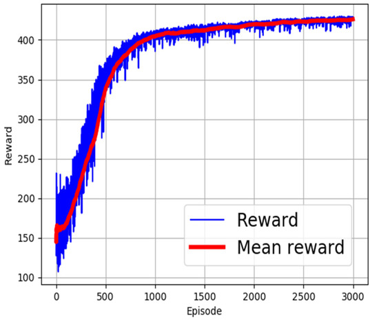
Figure 2.
Training with ReLU activation function.
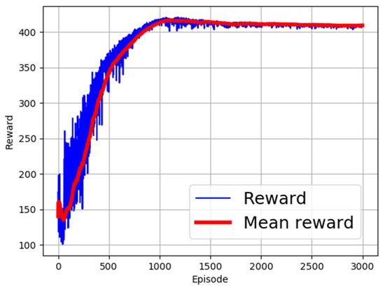
Figure 3.
Training with RBF activation function.
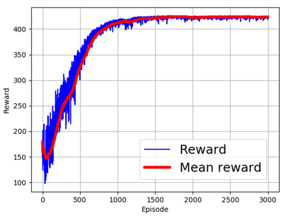
Figure 4.
Training with Sigmoid activation function.
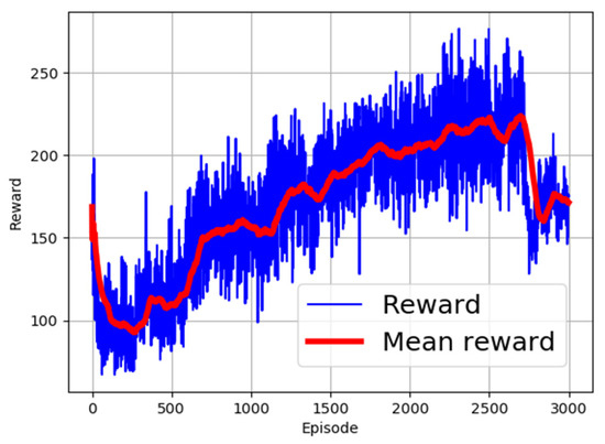
Figure 5.
Training with SoftMax activation function.
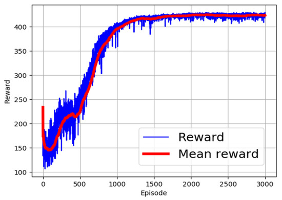
Figure 6.
Training with SoftPlus activation function.
The performance of tip position using RBF and ReLU is shown in Figure 7. From the figure, position in x-axis and z-axis are slightly different but position in y-axis is significantly different and does not improve over time. This implies that the tip did not arrive at the target position. In the figure, 1 point represents 50 episodes. This was plotted to improve visualization quality of the plotted data. During testing, the ReLU trained model was found to have the best performance and, hence, it is maintained as the activation function in the rest of the paper. The simplified activation function is shown in (8). In this case, the Adam optimizer is applied for stochastic gradient descent during training [34].
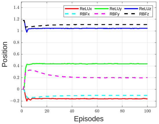
Figure 7.
Comparison of manipulator tip position with ReLU and RBF trained model.
3. Simulation of the Flexible Manipulator Model
To analyze the performance of the learning algorithm, robot simulator software was used to ascertain the position of the end effector with reference to the target. For this purpose, Multi-Joint dynamics with Contact (MuJoCo) physics simulator was used [35]. MuJoCo, produced by Roboti LLC® (Redmond, WA, USA), is free for students, and is a 3D physics engine developed for research and development in robotics targeting model-based optimization through contacts.
3.1. Actual Manipulator Model
To assess the RL outcomes for the flexible manipulator, a reference model was required. Figure 8a displays the physical implementation of the flexible manipulator used in the study, consisting of two links and three degrees of freedom for manipulation. The connection setup, including the boards and signaling components, is depicted in Figure 8b. For analog-to-digital conversion (ADC) and digital-to-analog conversion (DAC) processes, a dSPACE 1103 controller board was utilized. This board facilitated device driving and communication by converting analog signals to digital format and vice versa. The DC motor servo driver, connected to the dSPACE signal processing board, drove the motors responsible for manipulator movement. These motors were equipped with optical encoders, providing feedback on the angles of rotation with a pulse output of 1000 pulses per revolution. The angle information from the encoders was sent back to the servo drive amplifier and then transmitted to the dSPACE board. To reduce joint speed, harmonic drives were employed, effectively lowering the speed of the joints by a factor of 100. Specifically, Joint 1 exhibited twisting motion perpendicular to the ground, while Joints 2 and 3 allowed bending rotation. This configuration allowed the flexible manipulator to perform its intended movements and tasks.
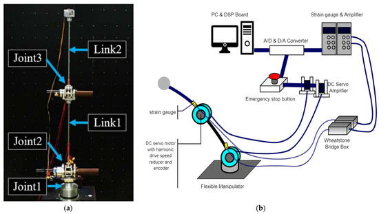
Figure 8.
Setup of the flexible manipulator. (a) Actual flexible manipulator, (b) illustration of the manipulator setup.
3.2. Virtual Manipulator Model
Figure 9 shows the schematic diagram of the proposed flexible manipulator. The design is inspired by a physical robot shown in Figure 8. From the figure, there are three motors (motor 1, 2, and 3) as shown. Motor 1 has z-axis rotation, while motor 2 and 3 have x-axis rotation. A mass with weight, w is attached to the tip, and the side length is h. There are two cylindrical rods which formulate Link 1 and Link 2 from the bottom. The length of each link (), diameter (), mass (), and the longitudinal coefficient () are listed in Table 4. Link 1 is assumed to be stainless steel, and Link 2 is assumed to be aluminum. Also, each link reproduces flexibility by connecting 11 cylinders with ball joints (Figure 10). Specific manipulator parameters are as shown in Table 4. Figure 11 shows the implemented design in MuJoCo, with the target object shown in red.
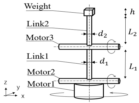
Figure 9.
Model of the flexible manipulator.
Table 4.
Parameters of the flexible manipulator.
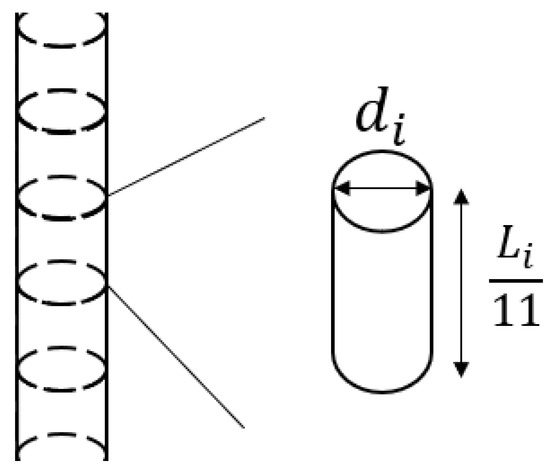
Figure 10.
Construction of the link.

Figure 11.
Proposed 3D Model of the flexible manipulator showing red target object.
The strain at the root of Link 1 is measured. A sensor that measures the force is attached 0.02 m above the root of Link 1. The strain in the y-axis direction, which is the out-of-plane direction, is parameter of consideration in this research. The calculation method of strain from the measured force is as shown in (9).
where M is the moment, given by (10):
The section modulus, can be written as shown in (11). In this case, d1 is the diameter of Link 1.
3.3. Experiment Setup
The flexible manipulator in the virtual and actual model is used to verify the performance. In the RL training phase, the target position shown in red (Figure 11) moves randomly within the reachable space of the manipulator. The distance between the tip of the manipulator and the target is used as a reward, in that the RL agent is rewarded for action-set that decreases the distance.
After training, the model is evaluated in an actual manipulator. For that, a predefined X, Y, Z position is supplied to the model as the target. The model outputs a corresponding input signal that is fed to each of the joints to realize the targets. For verification, the study also conducted an experiment where each joint is moved 20 degrees on the actual machine without the controller. This is the same end-effector position as that of the RL controller model. In the no-controller experiment, the manipulator starts with a vertical posture at t = 0.
Next, a characteristic comparison of the designed model with a physical two-link flexible manipulator used in the laboratory was performed. In a physical robot, when each motor is moved 20 degrees, the resonance frequency is 3 Hz for about 10 s until the vibration dies out for forward reverse motion. The steady strain is .
Figure 12 shows the modelled trajectory of the end effector of the designed model with no vibration control mechanism. Figure 13 is the Link 1 and Link 2 root strain response of the modeled and actual manipulators. The experimental and simulation results are in almost good agreement, and the modeling is considered valid. The performance is confirmed to have similar characteristics to the physical model reported in [36]. The model is designed to have a sampling rate of 0.002 s (1 step = 0.002 s).
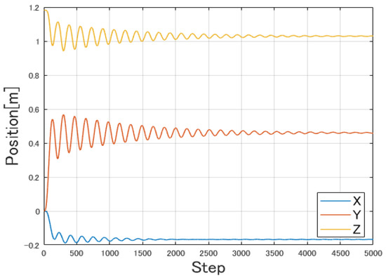
Figure 12.
Trajectory of end effector without vibration control.
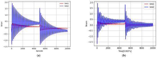
Figure 13.
Link 1 and 2 root strain responses. (a) MuJoCo model, (b) actual manipulator model.
4. Results and Discussion
The overall goal of the trained model is to control operations to bring the end effector closer to the target coordinates. If the target coordinate is at and the end effector coordinate is at , then the reward function R should be the distance between two points as shown in (12). The reward R is highest when the end effector is closer to the target coordinate and vibration is suppressed.
4.1. Position Control Results
Figure 14 shows the trajectory of the end effector after the learning phase. In this case, one episode is 500 steps. Compared with Figure 12, it can be seen that vibration has been suppressed. However, although the end effector is moved to the target position, it is clear from Figure 15 that strain has not been suppressed.
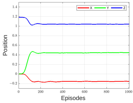
Figure 14.
Trajectory of end effector.

Figure 15.
Strain of Link 1 with learning phase.
4.2. Vibration/Strain Control Results
From Figure 14, the position of the tip of the flexible manipulator has been suppressed effectively with the exception of strain (Figure 15). To remedy for strain distortion, a new training model is performed where strain error is added to reward equations. The modified reward functions are shown in (13) and (14). The distortion amplification gain is set to The results of trained model data is shown in Figure 16 and Figure 17 for end effector position and strain, respectively.
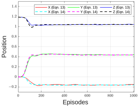
Figure 16.
Trajectory of end effector for Equations (12) and (13) (reward functions).
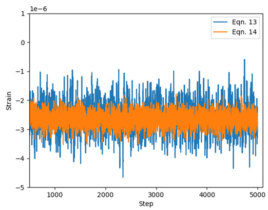
Figure 17.
Strain of Link 1 for Equation (13) and (14).
From the figures, both vibrations and strain were suppressed. As shown in Figure 17, the multiplicative model (Equation (14)) had better strain results compared to the additive model (Equation (13)). This is seen as a reduction in distortion (vibration) of the resultant strain. The magnitude of the target strain after reaching target coordinate was set in (12) to be . For (14), it was set at . Since (13) is an addition, it is argued that the overall reward increases as the distance from the target coordinate decreases. On the other hand, for (14), the distance from the target coordinate is short, and the total sum of rewards does not increase unless the distortion is suppressed. Equation (14) can be expressed as shown in (15).
Building from (15), the premise is that, as gain increases, the effect of the overall reward is propagated more, thereby reducing strain. To this end, was varied from , as shown in (14), to to arrive at an optimal gain for the reward function.
Figure 18, Figure 19 and Figure 20 show the results of the trajectories and strains for various values. From the results, the end effector reached the target coordinates in all reward functions. Notably, for higher values, slightly more time was needed before the position settled. This is as seen in Figure 17 where position of end effector in z-axis settles at around 300th episode for , compared with , which settles at approximately 150th episode.
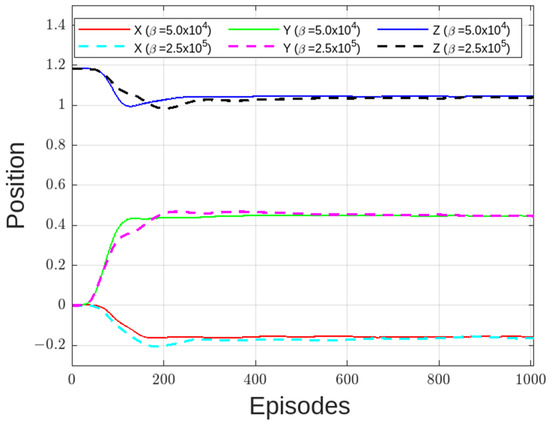
Figure 18.
Trajectory of end effector.
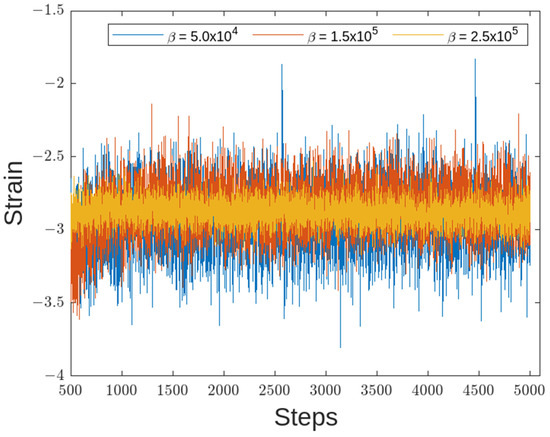
Figure 19.
Strain of Link 1 for β between 5 × 10⁴ and 2.5 × 10⁵.
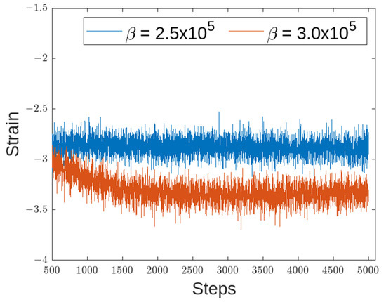
Figure 20.
Strain of Link 1 for β of 2.5 × 10⁵ and 3 × 10⁵.
Regarding the strain, different values of resulted in different strain suppressions, as shown in Figure 18 and Figure 19. When was made larger than the strain distortion diverged, as shown in Figure 20. This is considered to be the effects of distortions caused on the overall reward being too large. From the figure, Equation (15) with set to was considered the optimal reward function.
4.3. Experiment on the Actual Flexible Manipulator
Figure 21 shows the time response of the root strain voltage of Link 1, Link 2, and Link 3, respectively. From Figure 21, the joint angles did not converge to the target values. In addition, from Figure 22, the steady strain in the in-plane direction of Link 1 and Link 2 is the same, and vibration tends to be suppressed to some extent.
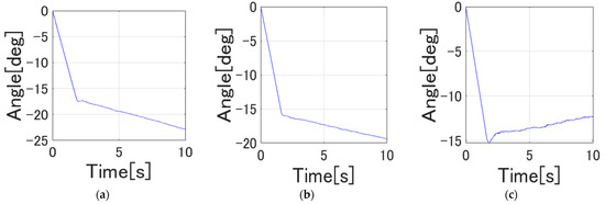
Figure 21.
Time response of the joints. (a) Joint 1 angle, (b) Joint 2 angle, (c) Joint 3 angle.
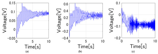
Figure 22.
Root strain response of the links. (a) Link 1 strain, (b) Link 2 strain, (c) Link 3 strain.
The power spectral densities of the strain at the base of each joint is shown in Figure 23. From the figure, we note that there are peaks around 3 Hz and 10 Hz, which are the resonance frequency components in the actual machine experiment similar to what is reported in [22,37]. By vibration mode analysis, among the resonance frequency components, the components near 3 Hz and 10 Hz are vibration modes in the driving direction of Joint 2 and Joint 3, and the components near 20 Hz are in the torsional direction, that is, in the torsional direction of Joint 1. It has been found that the vibration mode is in the rotational direction.

Figure 23.
Power spectrum of the links. (a) Link 1 strain, (b) Link 2 strain, (c) Link 3 strain.
Analyzing the changes in the distortion of Link 1 after applying reinforcement learning, as depicted in Figure 22, we observed favorable results in the numerical simulation. However, when implementing these learned policies on the actual machine, there is a possibility of encountering issues related to the motor’s ability to follow the desired trajectories. Previous research has indicated that subtle differences between the numerical simulation environment and the real-world experimental environment can significantly impact the learning outcomes in a negative manner, what is referred to as sim–real challenges [18,38,39].
The sim–real problem, characterized by the disparities between the simulated and experimental environments, likely played a significant role in the notable discrepancy observed between the modeled reinforcement learning outcomes and the experimental data. Some of the key causes of sim–real problems include:
- Model inaccuracies: The simulation model may not accurately capture all aspects of the real-world system, such as dynamics, friction, or other physical properties. Assumptions and simplifications made during modeling may have led to discrepancies when compared to the actual system;
- Sensor and actuator variability: Sensors and actuators used in the real-world setup may exhibit variations and uncertainties that are not adequately represented in the simulation. Differences in sensor accuracy, noise levels, actuator response, and other characteristics can contribute to deviations between the simulation and reality, leading to sim–real problems;
- Unmodeled dynamics and nonlinearities: Complex interactions and nonlinear dynamics within the system may not be fully captured in the simulation model. Structural deformations, coupling between joints, dynamic effects, and other unmodeled phenomena can result in discrepancies between the simulated and real-world behavior, leading to sim–real problems.
This emphasizes the need for further investigation through implementation experiments to thoroughly understand and address these challenges. By conducting additional research and experimentation, we hope to can gain insights into the specific issues arising from the sim–real problem and improve the adaptability and performance of RL model when applied to real-world systems.
5. Conclusions
In this paper, we successfully applied reinforcement learning to control the vibration of a two-link flexible manipulator. Through simulations of a 3D model in MuJuCo, we validated the position and vibration control, closely resembling our physical manipulator used in the laboratory.
During training, our objective was to minimize the distance between the end effector and target coordinates, incorporating displacement and strain into the reward function. To achieve this, we incorporated displacement and strain into the reward function using a multiplicative model (Equation (15)) with β set to 2.5 × 10⁵. The results demonstrated the effective suppression of vibration at the tip of the flexible manipulator, as well as mitigated strain distortions.
However, when applying the trained model to the physical manipulator, we encountered a sim–real challenge, resulting in a discrepancy between the simulation and experimental environments. This discrepancy may be attributed to modeling assumptions, sensor and actuator variability, environmental factors, calibration and setup differences, and unaccounted dynamics and nonlinearities.
To address these challenges in future studies, we propose remedies such as improving simulation fidelity, utilizing transfer learning techniques, iterative refinement through physical testing, and incorporating hardware-in-the-loop setups for real-time validation. By addressing the sim–real challenge and bridging the gap between simulation and reality, future research can achieve better alignment and enhance the robustness and reliability of flexible manipulator control using reinforcement learning.
Author Contributions
Conceptualization, M.S., F.K. and K.M.; methodology, J.M., F.K., D.M. and K.M.; software, F.K. and D.M.; validation, W.N., D.M. and K.M.; formal analysis, F.K., W.N. and K.M.; investigation, M.S. and D.M.; resources, M.S.; writing—original draft, J.M. and F.K.; writing—review and editing, J.M. and W.N.; supervision, M.S. and K.M. All authors have read and agreed to the published version of the manuscript.
Funding
This work is partially supported by Grants-in-aid for Promotion of Regional Industry-University-Government Collaboration from Cabinet Office, Japan.
Data Availability Statement
Not applicable.
Conflicts of Interest
The authors declare no conflict of interest.
References
- Khaled, M.; Mohammed, A.; Ibraheem, M.S.; Ali, R. Balancing a Two Wheeled Robot; USQ Project; University of Southern Queensland: Darling Heights, QLD, Australia, 2009. [Google Scholar]
- Sasaki, M.; Kunii, E.; Uda, T.; Matsushita, K.; Muguro, J.K.; bin Suhaimi, M.S.A.; Njeri, W. Construction of an Environmental Map including Road Surface Classification Based on a Coaxial Two-Wheeled Robot. J. Sustain. Res. Eng. 2020, 5, 159–169. [Google Scholar]
- Lochan, K.; Roy, B.K.; Subudhi, B. A review on two-link flexible manipulators. Annu. Rev. Control 2016, 42, 346–367. [Google Scholar] [CrossRef]
- Yavuz, Ş. An improved vibration control method of a flexible non-uniform shaped manipulator. Simul. Model. Pract. Theory 2021, 111, 102348. [Google Scholar] [CrossRef]
- Liu, Z.; Liu, J.; He, W. Dynamic modeling and vibration control for a nonlinear 3-dimensional flexible manipulator. Int. J. Robust Nonlinear Control 2018, 28, 3927–3945. [Google Scholar] [CrossRef]
- Njeri, W.; Sasaki, M.; Matsushita, K. Enhanced vibration control of a multilink flexible manipulator using filtered inverse controller. ROBOMECH J. 2018, 5, 28. [Google Scholar] [CrossRef]
- Uyar, M.; Malgaca, L. Implementation of Active and Passive Vibration Control of Flexible Smart Composite Manipulators with Genetic Algorithm. Arab. J. Sci. Eng. 2023, 48, 3843–3862. [Google Scholar] [CrossRef]
- Mishra, N.; Singh, S.P. Hybrid vibration control of a Two-Link Flexible manipulator. SN Appl. Sci. 2019, 1, 715. [Google Scholar] [CrossRef]
- Nguyen, V.B.; Bui, X.C. Hybrid Vibration Control Algorithm of a Flexible Manipulator System. Robotics 2023, 12, 73. [Google Scholar] [CrossRef]
- de Lima, J.J.; Tusset, A.M.; Janzen, F.C.; Piccirillo, V.; Nascimento, C.B.; Balthazar, J.M.; da Fonseca, R.M.L.R. SDRE applied to position and vibration control of a robot manipulator with a flexible link. J. Theor. Appl. Mech. 2016, 54, 1067–1078. [Google Scholar] [CrossRef]
- Liu, H.; Cheng, Q.; Xiao, J.; Hao, L. Performance-based data-driven optimal tracking control of shape memory alloy actuated manipulator through reinforcement learning. Eng. Appl. Artif. Intell. 2022, 114, 105060. [Google Scholar] [CrossRef]
- Roy, S.; Kieson, E.; Abramson, C.; Crick, C. Mutual Reinforcement Learning with Robot Trainers. In Proceedings of the 2019 14th ACM/IEEE International Conference on Human-Robot Interaction (HRI), Daegu, Republic of Korea, 11–14 March 2019. [Google Scholar]
- Kober, J.; Peters, J. Reinforcement Learning in Robotics: A Survey. In Learning Motor Skills; Springer: Cham, Switzerland, 2014; Volume 97, pp. 9–67. [Google Scholar] [CrossRef]
- Smart, W.; Kaelbling, L. Reinforcement Learning for Robot Control. In Proceedings of the SPIE; SPIE: Philadelphia, PA, USA, 2002; Volume 4573. [Google Scholar] [CrossRef]
- Wu, X.; Chi, J.; Jin, X.-Z.; Deng, C. Reinforcement learning approach to the control of heavy material handling manipulators for agricultural robots. Comput. Electr. Eng. 2022, 104, 108433. [Google Scholar] [CrossRef]
- Xie, Z.; Sun, T.; Kwan, T.; Wu, X. Motion control of a space manipulator using fuzzy sliding mode control with reinforcement learning. Acta Astronaut. 2020, 176, 156–172. [Google Scholar] [CrossRef]
- Qiu, Z.C.; Chen, G.H.; Zhang, X.M. Trajectory planning and vibration control of translation flexible hinged plate based on optimization and reinforcement learning algorithm. Mech. Syst. Signal Process. 2022, 179, 109362. [Google Scholar] [CrossRef]
- Sasaki, M.; Muguro, J.; Kitano, F.; Njeri, W.; Matsushita, K. Sim–Real Mapping of an Image-Based Robot Arm Controller Using Deep Reinforcement Learning. Appl. Sci. 2022, 12, 10277. [Google Scholar] [CrossRef]
- Ouyang, Y.; He, W.; Li, X.; Liu, J.-K.; Li, G. Vibration Control Based on Reinforcement Learning for a Single-link Flexible Robotic Manipulator. IFAC-PapersOnLine 2017, 50, 3476–3481. [Google Scholar] [CrossRef]
- Pane, Y.P.; Nageshrao, S.P.; Kober, J.; Babuška, R. Reinforcement learning based compensation methods for robot manipulators. Eng. Appl. Artif. Intell. 2019, 78, 236–247. [Google Scholar] [CrossRef]
- He, W.; Gao, H.; Zhou, C.; Yang, C.; Li, Z. Reinforcement Learning Control of a Flexible Two-Link Manipulator: An Experimental Investigation. IEEE Trans. Syst. Man, Cybern. Syst. 2021, 51, 7326–7336. [Google Scholar] [CrossRef]
- Njeri, W.; Sasaki, M.; Matsushita, K. Gain tuning for high-speed vibration control of a multilink flexible manipulator using artificial neural network. J. Vib. Acoust. Trans. ASME 2019, 141, 041011. [Google Scholar] [CrossRef]
- Nguyen, Q.C.; Vu, V.H.; Thomas, M. A Kalman filter based ARX time series modeling for force identification on flexible manipulators. Mech. Syst. Signal Process. 2022, 169, 108743. [Google Scholar] [CrossRef]
- Shang, D.; Li, X.; Yin, M.; Li, F. Dynamic modeling and fuzzy compensation sliding mode control for flexible manipulator servo system. Appl. Math. Model. 2022, 107, 530–556. [Google Scholar] [CrossRef]
- Ben Tarla, L.; Bakhti, M.; Bououlid Idrissi, B. Implementation of second order sliding mode disturbance observer for a one-link flexible manipulator using Dspace Ds1104. SN Appl. Sci. 2020, 2, 485. [Google Scholar] [CrossRef]
- Kober, J.; Bagnell, J.A.; Peters, J. Reinforcement learning in robotics: A survey. Int. J. Robot. Res. 2013, 32, 1238–1274. [Google Scholar] [CrossRef]
- Singh, B.; Kumar, R.; Singh, V.P. Reinforcement learning in robotic applications: A comprehensive survey. Artif. Intell. Rev. 2022, 55, 945–990. [Google Scholar] [CrossRef]
- Buffet, O.; Pietquin, O.; Weng, P. Reinforcement Learning. In A Guided Tour of Artificial Intelligence Research: Volume I: Knowledge Representation, Reasoning and Learning; Springer: Berlin/Heidelberg, Germany, 2020; pp. 389–414. [Google Scholar]
- Zhao, T.; Hachiya, H.; Niu, G.; Sugiyama, M. Analysis and improvement of policy gradient estimation. Adv. Neural Inf. Process. Syst. 24 2011, 26, 118–129. [Google Scholar] [CrossRef] [PubMed]
- Kubo, T. Reinforcement Learning with Python: From Introduction to Practice; Kodansha Co., Ltd.: Tokyo, Japan, 2019; pp. 140–166. [Google Scholar]
- Schulman, J.; Levine, S.; Moritz, P.; Jordan, M.I.; Abbeel, P. Trust Region Policy Optimization. In Proceedings of the 32nd International Conference on International Conference on Machine Learning, Lille, France, 7–9 July 2015. [Google Scholar]
- Wang, Y.; Li, Y.; Song, Y.; Rong, X. The influence of the activation function in a convolution neural network model of facial expression recognition. Appl. Sci. 2020, 10, 1897. [Google Scholar] [CrossRef]
- Nwankpa, C.; Ijomah, W.; Gachagan, A.; Marshall, S. Activation Functions: Comparison of trends in Practice and Research for Deep Learning. arXiv 2018, arXiv:1811.03378. [Google Scholar]
- Kingma, D.P.; Ba, J. Adam: A Method for Stochastic Optimization. arXiv 2014, arXiv:1412.6980. [Google Scholar]
- Todorov, E. MuJoCo: Modeling, Simulation and Visualization of Multi-Joint Dynamics with Contact; Roboti Publishing: Seattle, WA, USA, 2018. [Google Scholar]
- Sasaki, M.; Muguro, J.; Njeri, W.; Doss, A.S.A. Adaptive Notch Filter in a Two-Link Flexible Manipulator for the Compensation of Vibration and Gravity-Induced Distortion. Vibration 2023, 6, 286–302. [Google Scholar] [CrossRef]
- Mishra, N.; Singh, S.P. Determination of modes of vibration for accurate modelling of the flexibility effects on dynamics of a two link flexible manipulator. Int. J. Non. Linear. Mech. 2022, 141, 103943. [Google Scholar] [CrossRef]
- Ushida, Y.; Razan, H.; Ishizuya, S.; Sakuma, T.; Kato, S. Using sim-to-real transfer learning to close gaps between simulation and real environments through reinforcement learning. Artif. Life Robot. 2022, 27, 130–136. [Google Scholar] [CrossRef]
- Du, Y.; Watkins, O.; Darrell, T.; Abbeel, P.; Pathak, D. Auto-Tuned Sim-to-Real Transfer. In Proceedings of the 2021 IEEE International Conference on Robotics and Automation (ICRA), Xi’an, China, 30 May–5 June 2021; pp. 1290–1296. [Google Scholar]


Disclaimer/Publisher’s Note: The statements, opinions and data contained in all publications are solely those of the individual author(s) and contributor(s) and not of MDPI and/or the editor(s). MDPI and/or the editor(s) disclaim responsibility for any injury to people or property resulting from any ideas, methods, instructions or products referred to in the content. |
© 2023 by the authors. Licensee MDPI, Basel, Switzerland. This article is an open access article distributed under the terms and conditions of the Creative Commons Attribution (CC BY) license (https://creativecommons.org/licenses/by/4.0/).