Abstract
Jointing Condition-Based Maintenance (CBM) with the Proportional Hazards Model (PHM), asset-intensive industries often monitor vital covariates to predict failure rate, the reliability function, and maintenance decisions. This analysis requires defining the transition probabilities of asset conditions evolving among states over time. When only one covariate is assessed, the model’s parameters are commonly obtained from expert opinions to provide state bands directly. However, the challenge lies within multiple covariate problems, where arbitrary judgment can be difficult and debatable, since the composite measurement does not represent any physical magnitude. In addition, selecting covariates lacks procedures to prioritize the most relevant ones. Therefore, the present work aimed to determine multiple covariate bands for the transition probability matrix via supervised classification and unsupervised clustering. We used Machine Learning (ML) to strengthen the PHM model and to complement expert knowledge. This paper allows obtaining the number of covariate bands and the optimal limits of each one when dealing with predictive maintenance decisions. This novel proposal of an ML condition assessment is a robust alternative to the expert criterion to provide accurate results, increasing the expectation of the remaining useful life for critical assets. Finally, this research has built an enriched bridge between the decision areas of predictive maintenance and Data Science.
Keywords:
Physical Asset Management; CBM; PHM; condition assessment; machine learning; clustering; k-means 1. Introduction
Data-driven decisions for complex equipment and its critical components are essential for optimal system performance, thereby meeting the premise of success for asset-intensive industries. This premise can be met through Physical Asset Management (PAM). PAM focuses on a sustainable outcome through equipment productivity—considering, for example, the establishment of an optimal maintenance policy that allows for reaching the goals desired for such equipment, whether these are to maximize availability or minimize costs, or others.
Among the maintenance policies, one of the most interesting is predictive maintenance, which defines the most suitable moment for intervention for a piece of equipment to minimize the probability of failure through diverse techniques. Condition-Based Maintenance (CBM) can be used as a predictive policy to estimate equipment failure rate and reliability based on current and future conditions. This is achieved through constant monitoring of these conditions and the use of tools such as the Proportional Hazards Model (PHM), which assigns a weight to each condition to then calculate the failure risk of the equipment at that moment. Moreover, this information needs to be complemented to decide on the intervention of the asset; the different values of the failure risk that determine when keeping the equipment operating is acceptable and when to conduct maintenance need to be determined; i.e., certain ranges that define the different possible decisions should be established.
Jointing CBM with PHM, it is possible to monitor vital signs or covariates to predict failure rate, reliability functions, and maintenance decisions. This analysis requires defining the transition probabilities of asset conditions that evolve over states, over time. When only one covariate is being assessed, the model’s parameters are commonly derived from expert opinion to provide state bands directly. However, the challenge lies in multi-covariate problems, where arbitrary judgment is inappropriate, since the composite measurement does not represent any physical magnitude. Moreover, selecting covariates requires more procedures to prioritize the most relevant ones.
Currently, there is no default method that accurately and systematically calculates the ranges or status of the equipment for different contexts and conditions. Therefore, in this study, a model is proposed that comprises a method for calculating them using different Machine Learning (ML) algorithms, which use historical information of equipment condition, interventions, and failure. Consequently, the present work aimed to determine multiple covariate bands for the transition probability matrix by supervised classification and unsupervised clustering. We used ML to strengthen the PHM model and complement expert knowledge. Furthermore, this paper allows obtaining the number of covariate bands and the optimal limits of each one when dealing with PHM-CBM predictive maintenance decisions.
In summary, we introduce a new contribution in terms of formulation, analytical properties, and practice for multiple covariate problems, whose bands have a combined measurement unit that often does not represent any physical magnitude. Therefore, to the best of our knowledge, using non-arbitrary criteria for multi-covariate bands has yet to be addressed in depth. Here is when our novel proposal for a CBM-ML condition assessment comes into play, expecting to be of value to asset managers.
This work is divided as follows: In Section 2, the different concepts applied in the model and a literature review are introduced. In Section 3, the proposed model and methodology are presented. Section 4 addresses a case study in which the model is applied. Then, the results of the case study are discussed. In Section 5, the conclusions of this work are presented.
2. Literature Review
2.1. Physical Asset Management
In recent years, Physical Asset Management, or PAM, has become a key element for asset-intensive industries. Mining, aeronautics, defense, and other capital-equipment firms are increasingly looking for more efficient and safer methods to perform operations and aiming for mechanisms to integrate with maintenance decisions [1,2,3]. The development of PAM has been marked by the need for a comprehensive approach, optimizing equipment’s value across its life cycle and explicitly using and implementing an Asset Management System (AMS)—that is, recognizing value for the business, reducing risk, and reducing the whole-life cost of assets [4].
The revolution of Industry 4.0 gives us the opportunity to manage asset costs, risks, and performance comprehensively [5]; more than ever, industries can use advanced tools such as predictive analysis or artificial intelligence to monitor and predict the performances of assets and processes [6]. According to [5], the whole AMS could be developed with these tools. Therefore, the industry requires innovative approaches to cope with these evolving challenges.
2.2. Condition-Based Maintenance
Condition-Based Maintenance, or CBM, allows for making maintenance decisions based on information collected through the monitoring of asset conditions [3,7]. This preventive maintenance technique employs the monitoring multiple parameters, such as vibration, contaminants, and temperature, to predict failure, improving the management of asset health and reducing the cost of their life cycles. The work of [4] proposes that condition monitoring is one of the factors considered in the basic practices of PAM, which is also important for the development of an AMS with a comprehensive approach.
In order to contrast the specific contributions to the present work, some recent and relevant CBM studies are indicated as follows. The work of [8] addresses CBM scheduling for a continuously monitored parallel manufacturing system with units subject to deterioration. They use a framework with a bivariate continuous-time Markov process (birth/birth-death process) to model the production system’s state transition. Nonetheless, the states of units are given, and the deterioration process is equal for all. The work of [9] states the preferences of a risk-averse decision maker for the CBM policy optimization, so the risk tolerance is traded off with the potential outcomes of the maintenance policy in order to optimize the CBM policy. The proposed method takes care of an engaging problem, although the parameters and variables are deterministic. In [10], a CBM policy with dynamic thresholds and multiple maintenance actions for a system subject to periodic inspection is proposed; the thresholds are used to decide when to perform a particular maintenance action. One of the most prominent aspects of this paper is incorporating the proportional hazards model with a continuous-state covariate process to describe the hazard rate. The dynamic limits are determined by using a semi-Markov decision process framework. However, these thresholds are defined based on heuristic covariate bands to discretize the Markov chain’s states, with an equal range among them.
The Proportional Hazards Model, or PHM, works as a statistical procedure for estimating the failure risk of a piece of equipment based on condition-monitoring information [11,12]. The PHM’s baseline hazard function has been widely used as a Weibull distribution due to its flexibility and closed-form risk and reliability function [13,14]. Ref. [15] presents a method for calculating reliability and remaining useful life (RUL) based on current conditions. a single covariate. Then, data are discretized in different states, such that various reliability functions, representative of each state, are calculated. These reliability functions are depicted graphically, showing the differences in their die-off rates. Finally, the authors of [12] developed software aimed at optimizing CBM for the decision-making process of asset intervention. The software comprises multiple covariates, transition probability matrices, PHM and the costs associated with corrective and preventive interventions.
2.3. Machine Learning Approach
One of the relevant aspects this study attempted to develop is the integration of Machine Learning, or ML, into models aimed at establishing intervention policies, thereby being asset management to Industry 4.0. The use of ML and data management is one of its main pillars [16].
Generically speaking, ML can be understood as the use of algorithms that learn from experiences as a human being would do [17]. In the case of these algorithms, experience is directly related to data, i.e., by showing them (or not) what to search for (supervised and unsupervised learning), or by “punishing” and “rewarding” them during learning (reinforcement learning) [18].
Among unsupervised learning algorithms, the clustering algorithm family seeks to group a dataset according to shared similar characteristics, making them as different as possible from other groups or clusters [19]. There are several approaches and ways of performing clustering. In this study, we used partitional clustering (PC) and model-based clustering (MC). PC is characterized by algorithms with a default number of clusters being generated, in which each observation belongs to only one cluster [20,21]. MC algorithms first create a primary model to identify the statistical distribution parameters of each cluster, and from them, classify observations within these clusters [20,21].
One of the most widely used PCs algorithms is k-means [20,22]. This algorithm, proposed by Stuart Lloyd (1982) [23] and Edward W. Forgy (1965) [24], finds k-clusters by minimizing the squared root of the sum of the distances from each point to the corresponding centroid of its cluster [25]. It consists of two phases: first, the centroids of each cluster are identified, and second, each observation is classified according to its distance from each centroid [22]. Due to its iterative optimization process, convergence is fast, which is one of the factors that make it a popular algorithm in ML [26]. K-means has been used to improve urban zoning for cargo logistics [27], image segmentation [22], and urban flood risk mapping [28], among others [29].
The Gaussian mixture model (GMM) is an MC algorithm widely used in diverse areas such as image segmentation, signal processing, and biomedical sciences [21,30]. GMM has the capacity to make mild approximations of general functions of probability density through weighted sums of multiple Gaussian functions [31]. In addition, GMM does not only provide a uniform generalized distribution adjustment, but its components (or clusters) can clearly describe multimodal density if necessary [32]. Therefore, it can be used to predict and classify data by associating them with different components based on probability distributions [33].
An aspect to consider in k-means and GMM is their dependence on a hyper-parameter k that represents the number of clusters the algorithm has to generate; consequently, the challenge in using them is to find the optimal k value [28]. In general, these problems are solved by evaluating different k values and comparing their performances with validation indexes [34], such as silhouette [19,27,28], the elbow method [29], the Akaike information criterion [30,35] or the Bayesian information criterion [21,35]. They can also be solved using visual methods [34], such as dendrograms [36]. However, the nature of the problem to be solved should always be kept in mind.
The previous paragraph highlights a relevant element of this study; after calculating the centroids generated through k-means and the probability distributions extracted from GMM, states (clusters) and their covariate bands (ranges of covariate values describing a certain state [37]) are expected to be determined. They are both necessary for the creation of the transition probability matrix that, in turn, is required for the development of PHM.
2.4. ML Applications in CBM
In order to improve the CBM strategies, some studies have used different ML techniques. For example, ref. [38] proposed a CBM strategy considering dynamic maintenance policies. The optimization model involves a Markov decision process improved by neural networks and Q-learning (reinforcement learning), also known as deep-Q learning (DQL). Nevertheless, the state thresholds are defined arbitrarily. The work reported in [39] developed a semi-supervised, clustering-based framework for maintenance decision-making based on Cox’s PHM model [11]. They used k-means to estimate the state of the system based on its age and the values from the condition monitoring. The state-space with its associated transition probability is defined based on clustering. This contributes to developing an innovative methodology and estimating the system’s state without expert knowledge. However, the parameter k is randomly established, and the k-means algorithm can have problems with robustness against outliers and edge cases.
3. Model Formulation
3.1. Data Pre-Processing
First, treating data prior to their use is critical, i.e., to ensure the absence of null, missed, or duplicate data. Additionally, different tables are integrated in order to have all the available information in a single document.
In turn, it is important to identify types of maintenance and classify them using a binary system for their subsequent use in the model, in which one and zero correspond to preventive and corrective maintenance, respectively.
The difference in days between each intervention is obtained, and NaN data are treated, yielding two cases:
- Completing the NaN values with the following value if data follow a certain trend.
- Completing NaN values with data averages.
This generates a table with only data relevant to the development of the model, i.e., with dates, an identifier for assets and their components if existent, the type of intervention in the binary system, the difference of days between interventions and a column for each covariate.
3.2. Parameters Estimation
The and parameters represent the stages at which the asset and its characteristic life are, respectively. To estimate them, the reliability of all data should be estimated first. In this case, it is obtained through the Lewis method:
where is a binary variable that takes the value 1 when a censure occurs (e.g., preventive interventions) and 0 when a failure happens. Then, reliability is calculated as a function of time, as proposed by Jardine (1987) [13], who indicated that reliability can be model as a two-parameter Weibull distribution through:
By linearizing the aforementioned expression, the following equation is obtained:
where is the shape parameter (slope) and is the scale parameter.
3.3. Data Division and Standardization
The following step corresponds to the division of the database into two groups: a training group and a testing group. This division is mainly necessary for using machine learning algorithms, as they require previous training before delivering final data. In this way, the training data group will be used with this purpose, and the testing group will be employed to obtain valid results from these algorithms.
There is not a single rule for the quantity of data that should be left in one group or another, but the division of the whole database into 3/4 for the training group and the remaining data for the testing group is customary.
In turn, before working on covariates data, it is recommended to standardized the data. This implies re-escalating the data in such a way that they have the same order of magnitude among them, as well as the same minimum and maximum values. This facilitates the analysis of the weights of each covariate, as they can be compared directly, allowing for establishing their relative importance to one another.
3.4. Covariates Weight Calculation
Before conducting the clustering of the , their corresponding weights should be calculated with respect to the failure rate associated with each sample from the database. To calculate them, this work proposes using a random forest algorithm, which receives the values of each covariate and their corresponding failure rates (obtained in the previous step) as input parameters. With this, the algorithm delivers the relative importance of each z with respect to its failure rate, which will be used as their respective weights.
It should be noted that, since this algorithm has diverse options in terms of hyper-parameters to enter prior to its use, it is recommended to test different combinations of the same and define which of them yields the best results for the database. This can be conducted automatically with different code commands associated with machine learning.
It is noteworthy that the calculation of the weights of the different is not the focus of this work, and therefore this procedure is solely used to obtain values related to the database under use and move to the following steps of the proposed model. The validity of the weights obtained through this algorithm has not been proven; thus, in cases of needing to calculate them, other proven alternatives are recommended.
Once the weights are obtained, a new parameter is introduced into the database, which will be used for cluster division. This corresponds to the sum of of each covariate; i.e.:
3.5. Clustering
To use the clustering algorithm, data simplification is recommended, which is—in this case, —subdivided into class intervals. Intervals will be assigned their corresponding class mark, which reduces the quantity of data the algorithm has to work with. To determine the number of intervals into which the database is divided, Sturges’ rule is employed, which is based on the number of samples to define the intervals.
Afterwards, this work proposes two different clustering algorithms, one through k-means and the other one through the Gaussian mixture model (GMM). The main hyper-parameter that both methods require is the number of clusters into which data are hoped to be divided. To determine this number, different numbers can be input and the results compared to select one of them, as conducted with the random forest. Among the aspects to consider for this choice are the different values yielded by the algorithm, such as the silhouette index mean or Akaike values (BIC and AIC), which allow for comparing the results to decide what number of clusters better adapts to the database. In turn, it should be kept in mind that the selection of simpler models is always recommended; i.e., if the difference in the adaptation between two numbers of clusters is low, the cluster that divides data into a number of clusters much smaller is preferred. What these clusters will represent in the analysis to be performed should also be considered, as it may provide some clues about the most realistic number of clusters for a specific case. The number of class intervals into which data were divided at the beginning should not be overlooked, because it is likely that if these are divided into the same number of clusters, the results of such division may be biased and not necessarily be the best option.
Finally, once the number of clusters is selected and the database is divided via the algorithms mentioned above by means of their corresponding parameters, the last step is to classify/mark each datum in the cluster to which it belongs in order to facilitate the observation of the algorithm’s result.
3.6. Covariate Bands- Calculation
The covariate-bands calculation is performed using the following steps:
- Through distance to centroids: Based on the clustering by GMM and k-means, the centroids of each cluster are calculated; then, the average between successive centroids (i.e., average between 1 and 2, 2 and 3, etc.) is calculated to define these values as limit ranges. In this way, a range value indicates in which cluster each will be found.
- Through probabilities: Using the found clusters, the probability that each observation belongs to this cluster is calculated to classify them. Then, the minimum values of each value belonging to each cluster are identified, and these delimit the ranges.
- Cluster border classification methodology: In cases where the value is close to one of the classification borders and elucidating what cluster it belongs to is not easy, a solution using the probabilities given by GMM is proposed. If the value has a difference smaller than 5%, a random choice is applied using the probabilities of belonging to each cluster, i.e., how likely it is that a certain value belongs to one cluster or another.
3.7. Transition Probability Matrix
Once ranges are calculated, the next step is to generate a transition probability matrix. To this end, the state to which each database sample belongs should be identified. Then, ordering the database chronologically, state transitions are identified, specifically how many times one state i transited to a state j, for all possible state combinations. This value will be identified with the parameter . Subsequently, the following parameter to be calculated is , which represents the time for which the equipment remains in state i. With these two parameters, the transition rates are calculated based on the expressions below:
Finally, transition probabilities are calculated as follows:
3.8. Reliability Calculation
At this step, the quantity of iterations to conduct is first established, for which an initial value for time and a value for the span between the initial and final value of time is required, as the lower the value, the more precise the result will be. Then, the number of iterations performed is:
Subsequently, the exponent value of each covariate () should be obtained through:
where is the weight of each covariate and is the approximation interval length. The values obtained through the previous equation are expressed in a diagonal matrix and then multiplied with the transition probability matrix, which should also be expressed in a diagonal matrix, thereby obtaining matrix L.
The following step is to obtain the product between L from the previous iteration and the current iteration. The conditional reliability is obtained through the sum of each row of the last matrix. This is conducted using the product-property method explained in detail in [15], for which the failure rate matrix is first estimated through the equation:
Using the above together with the transition probability matrix, the matrix and L are finally solved.
4. Case Study and Discussion
In this case study, the methodology presented in the previous section was used in a sample of 100 machines, each of them with four components. The critical components of interest can be assimilated as the electric motor stator of a fleet of haul trucks operating in a mine site. The voltage, rotation, pressure, and vibration of each component were measured, these being the covariates examined.
Regarding data pre-processing, the absence of null and duplicate data was first confirmed. Then, data were classified using a binary system into having preventive maintenance (1) or corrective maintenance (0). Afterwards, NaN values were completed using the following value, since, in this case, the use of data average may affect results due to data behavior. Table 1 shows an extract of the 100-machine sample.

Table 1.
Extract of the case study’s data.
In Table 1, it is possible to appreciate that the different columns correspond to various data related to the main groups: time and covariates. The first is the date on which the measurement of the covariates was carried out. Next, the Machine ID identifies which machine the analyzed component corresponds to. Then, the type of component is determined, and subsequently, the type of intervention, if it has been corrective or preventive. The time elapsed between interventions allows for estimating how long the component has been available, and finally, the individual measurements of the covariates. Voltage has been measured in V, rotation in rpm, pressure in Pa, and vibration in Hz. It is important to remember that although each covariate must work within a well-defined interval, the combined effect of all of them works as an indicator to define the status of the component and as a consequence of the corresponding machine. This last effect leads to a significant purpose of this manuscript: the proposal of an ML condition assessment to complement the expert criterion when dealing with multiple covariates and diverse measurement units.
In turn, to facilitate the use of data, a new table was created for each component to address them separately. In this case, only component 2 was used because it had the greatest amount of data, and the development of the other components is analogous to this one. Subsequently, as mentioned in Section 3.2, parameters and were estimated, obtaining the values presented in Table 2.

Table 2.
Parameters and for each component.
To confirm that such values are correct, reliability was calculated by Equation (2), where t is now a test time interval; in this case, time intervals that increase in 10 units were used. The value of should match with the time interval in which reliability is approx. 37%.
The next step after confirming the results was data division and standardization. In this case, as mentioned during formulation, the database was divided into a training group, which was composed of 572 samples, and a testing group with 191 data points. Then, covariates were standardized in a 0.01–0.1 range, selecting these values to avoid zero and negative numbers, as these could alter the results. Subsequently, the weights of the covariates were calculated (rotation, pressure, voltage, and vibration) with respect to the failure rate using the random forest algorithm, obtaining the parameters through Equation (4).
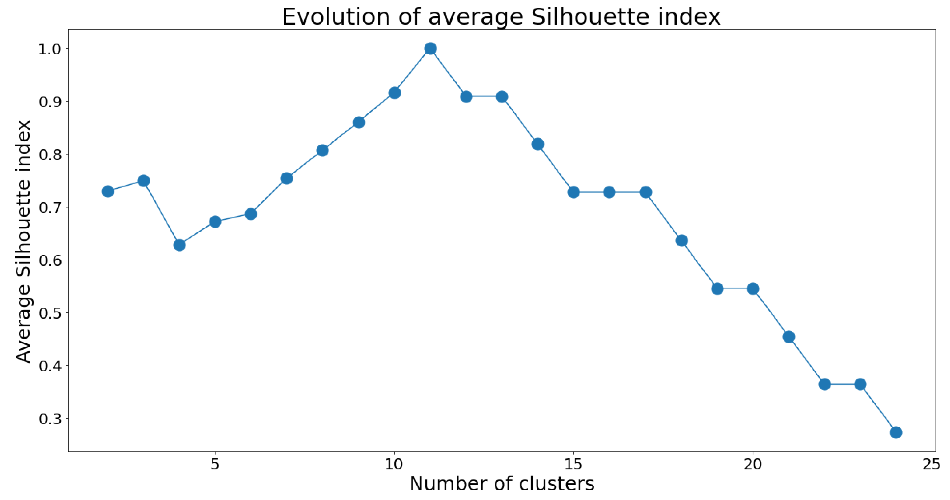
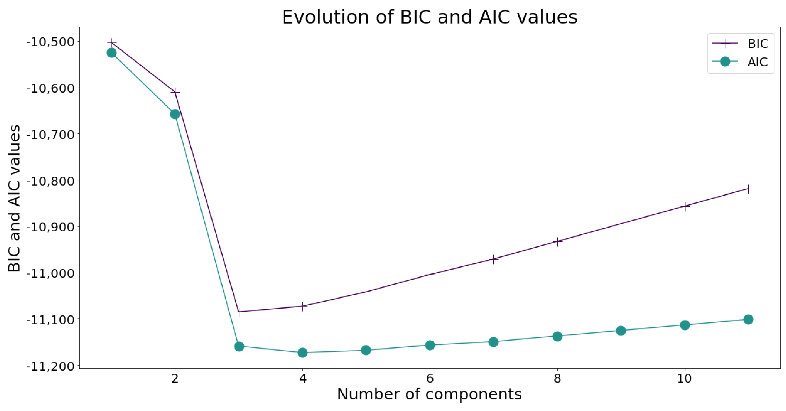
In addition, data was divided into class intervals by means of Sturges’ rule, which yielded 11 intervals. After the above procedure, the two clustering methods of k-means and GMM were employed to define the number of clusters that better adapt to the database. In both cases, the result is 3, which was obtained from the results shown in Figure 1 and Figure 2.
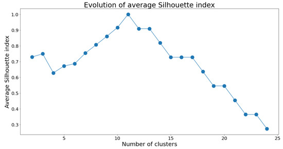
Figure 1.
Evolution of silhouette indexes’ means for different cluster numbers of the k-means method.
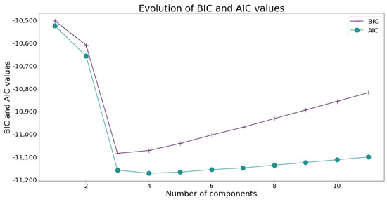
Figure 2.
Akaike values (BIC and AIC) for different cluster numbers of the GMM method.
The figures above show that the results of methods are similar for this database. In this way, the limits of each cluster were generated, which in turn define the states of the component. Different methods are proposed to achieve this.
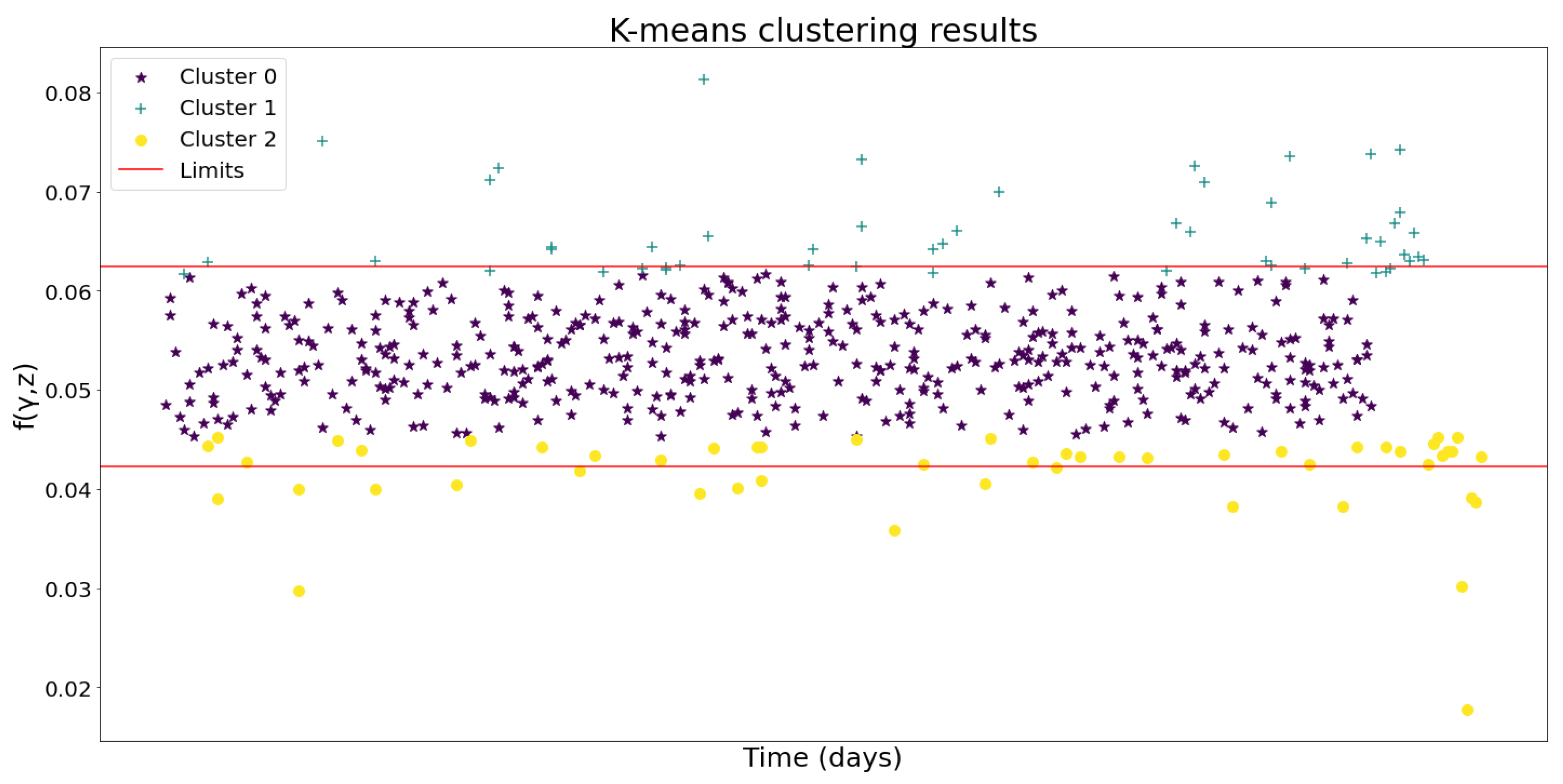
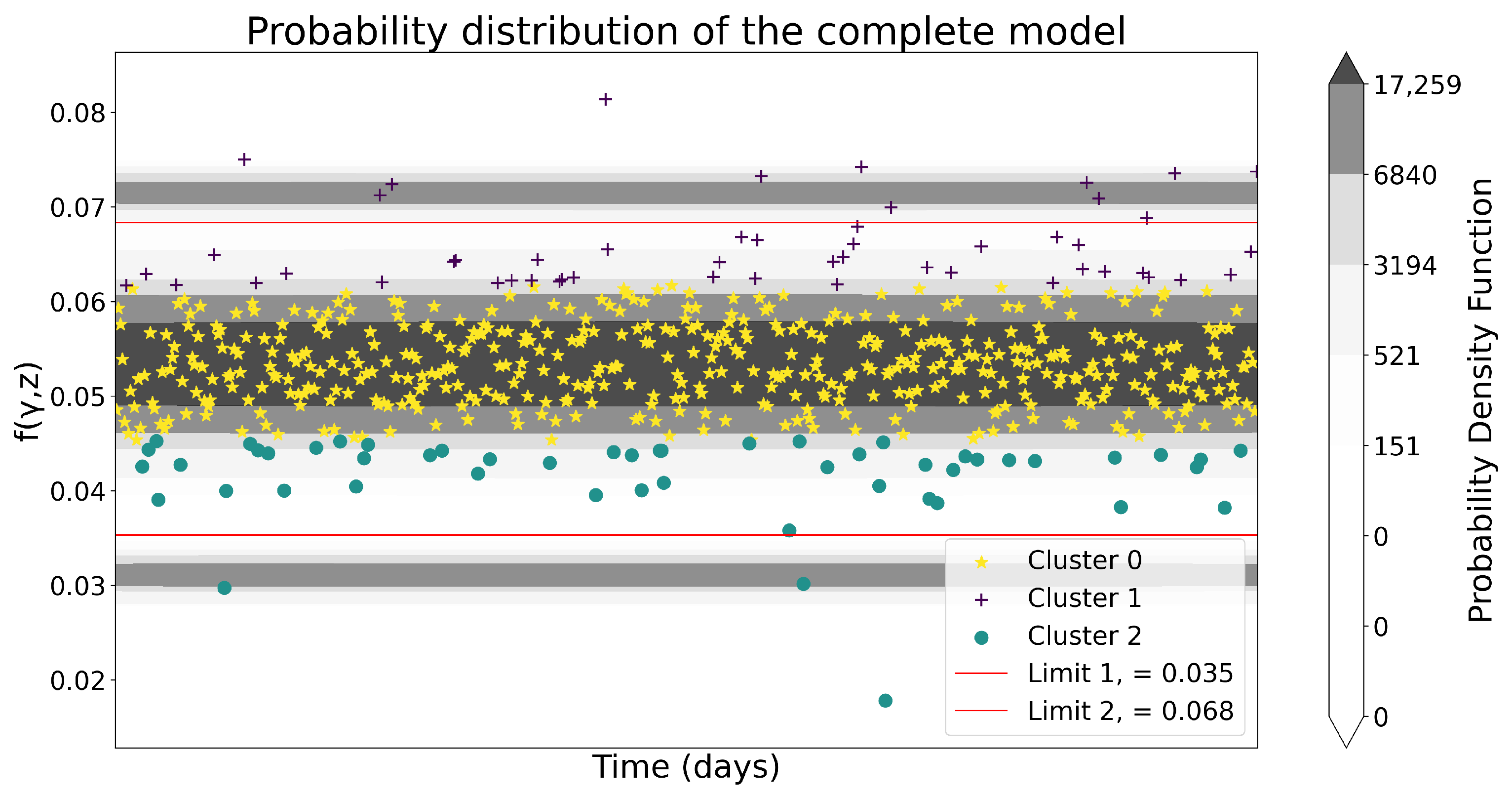
The first one is through the centroids of each cluster. The limits between two clusters are defined as the medium points between both centroids, which are presented in Figure 3 and Figure 4, for each k-means and GMM, respectively.
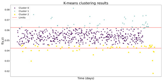
Figure 3.
Number of clusters obtained through k-means.
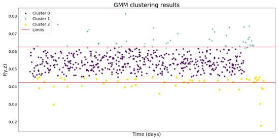
Figure 4.
Number of clusters obtained through GMM.
From this point, only the GMM method was employed. Table 3 specifies the numerical limits for data training, and the results of Table 4 were used for data testing.

Table 3.
States/clusters with training data.

Table 4.
States/clusters with testing data.
The second method for calculating the ranges of each state was based on the probabilities delivered by the GMM method. These can be graphically observed in Figure 5.

Figure 5.
Sum of over time and its probability density distribution of the complete model.
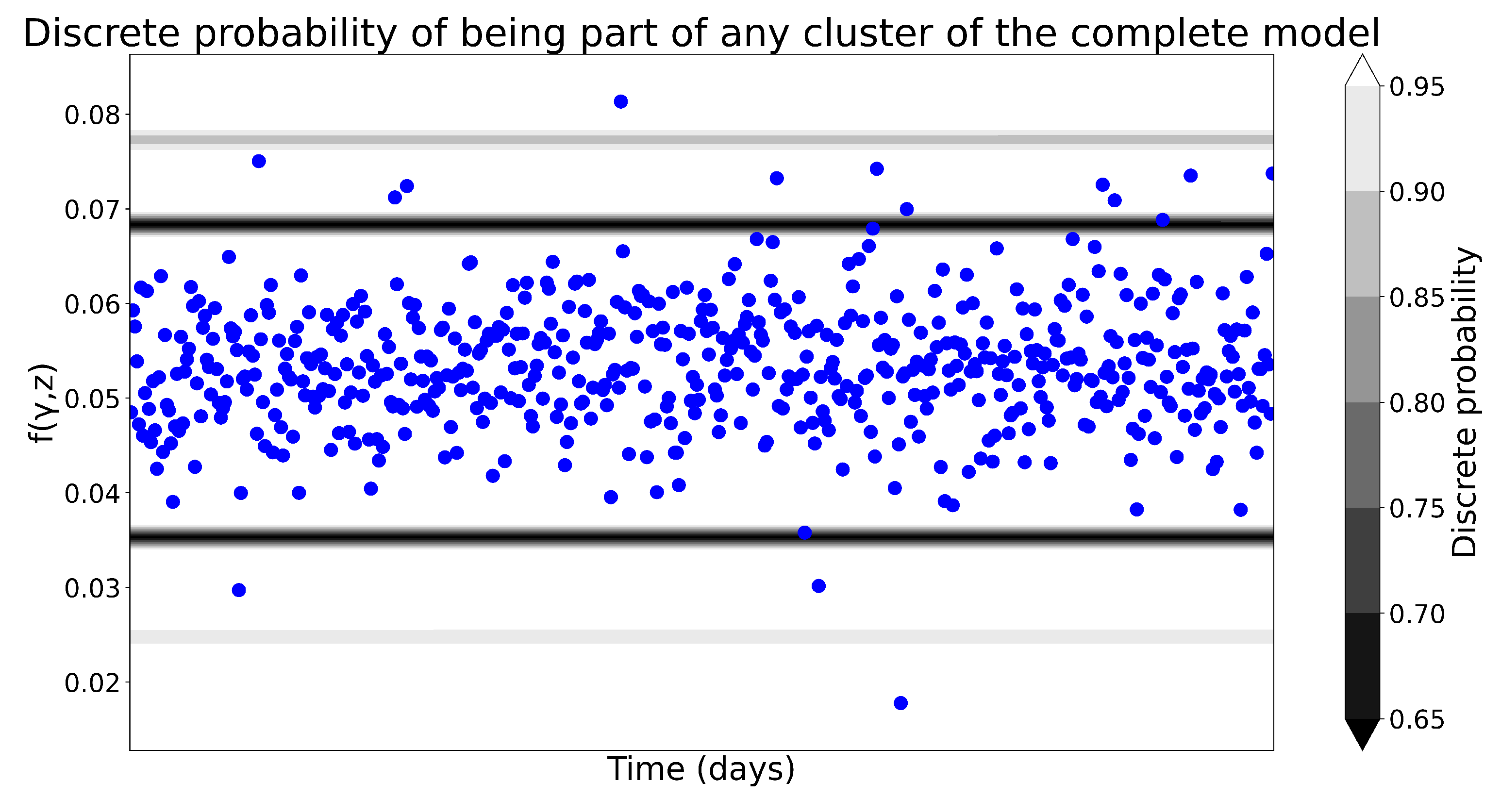
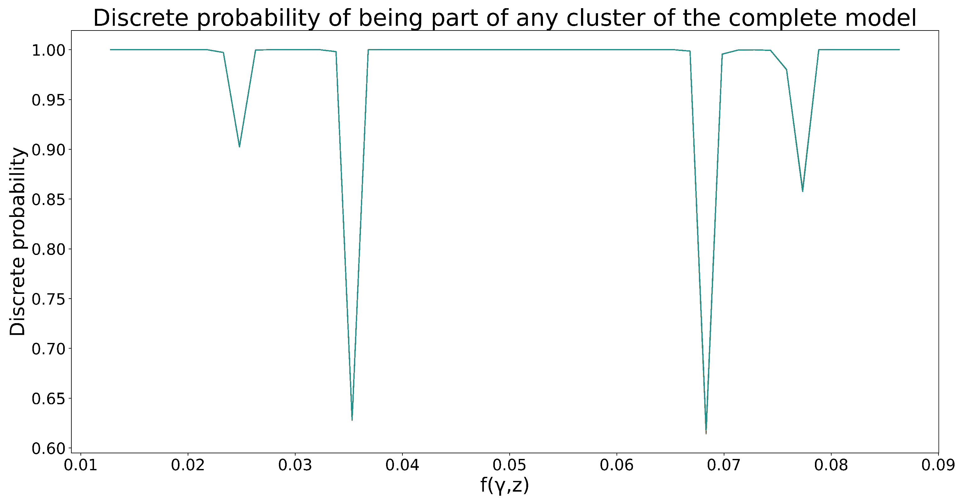
In this case, limits are defined as the lowest point of the probability of belonging to a cluster, which is depicted as darker areas in Figure 6. In Figure 7, the two lowest points that will define these limits are also clearly observed.
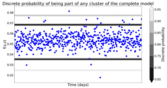
Figure 6.
Distribution of over time and its discrete probability of belonging to a cluster of the complete model.
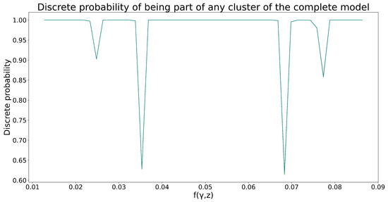
Figure 7.
Sum of over time and its discrete probability distribution of belonging to a cluster of the complete model.
Regarding the results for range calculation, both methods reached similar yet not equal results. This work does not focus on analyzing the advantages or disadvantages of one method over another. From this point, the calculations continued based on the range results obtained by probability.
When classifying each sample into its corresponding state, 557 data points were obtained that belonged to state 2 (central cluster), 12 to state 3 (upper cluster), and 3 to state 1 (lower cluster).
As an alternative result, it is considered that probabilities of belonging to one cluster or another are less clear for points close to the limit between clusters; therefore, a reliability range around this limit is proposed such that if the differences in probabilities of belonging between clusters is smaller than 5%, a point within this range is randomly classified into another cluster with equal probabilities of belonging to this limit. In this way, the quantity of data for this cluster becomes:
- state 1 = 3 data
- state 2 = 550 data
- state 3 = 19 data
Subsequently, the probability transition matrix—in Table 5 and Table 6 for training and testing data, respectively—was calculated using the results obtained with this last method.

Table 5.
Probability transition matrix with training data.

Table 6.
Probability transition matrix with testing data.
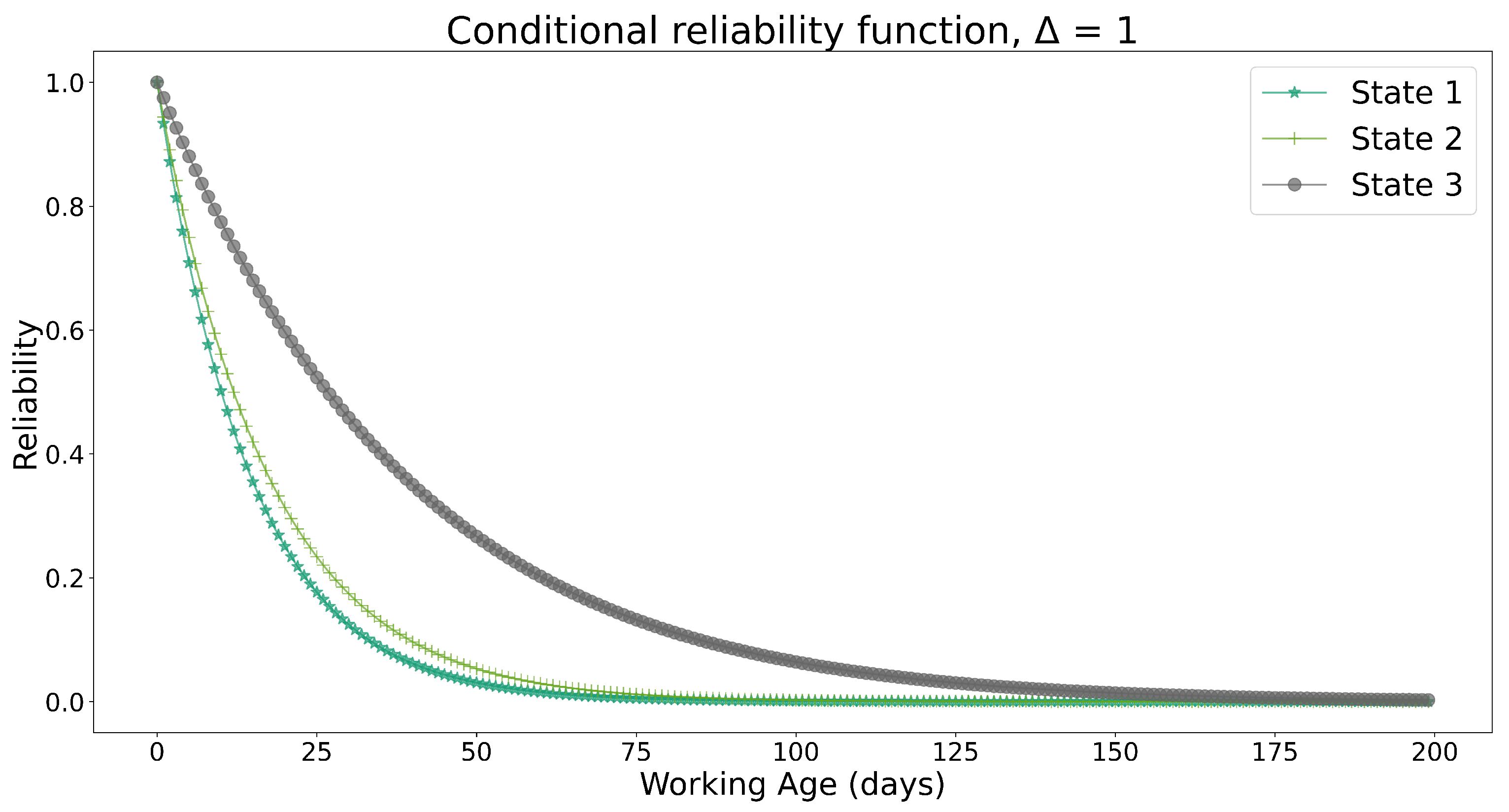
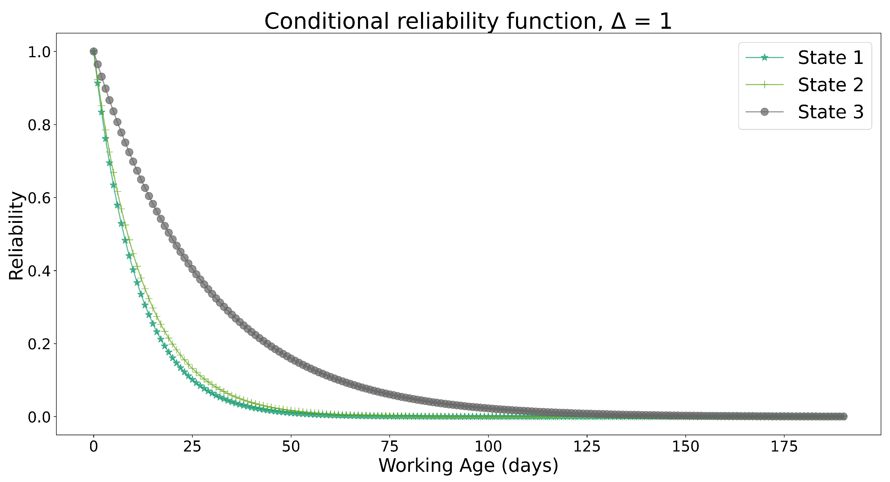
Finally, the conditional reliability function is estimated through the steps described in Section 3.8. In this case, it is established that is 360 and is 1. Then, reliability with respect to time was obtained for both training and testing data. Figure 8 and Figure 9 present the corresponding conditional reliability functions using the probability transition matrices as input to the aforementioned product-property method.
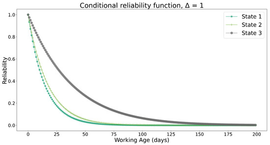
Figure 8.
Conditional reliability function with training data.
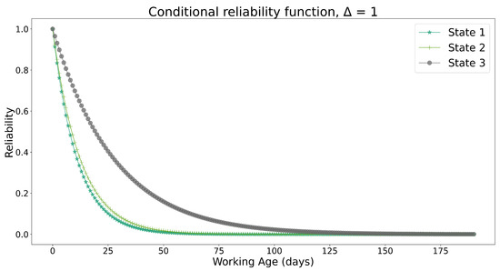
Figure 9.
Conditional reliability function with testing data.
These figures show that, for both cases, the reliability behavior for each state was similar. Specifically, it can be determined, based on the same, that state 3 corresponds to the state in which the component exhibited the highest reliability, followed by state 2 and then state 1, which presented the lowest reliability over time. This agrees with the quantity of data present in each state. This data analysis consisted of 100 machines with four components each and was aimed at defining the limit ranges of multiple covariates. The results obtained after pre-processing data to establish the treatment of NaN, null, or duplicate data were the estimates of parameters and using the Lewis and Jardine methods. Since the quantity of data associated with component 2 was larger, this was the selected component (considering that each piece of equipment has this component), obtaining and (days).
Once these parameters were obtained, data were divided, allocating 3/4 of them—572 data points—to the training of machine learning algorithms and 1/4—191 data points—to validation using those algorithms. In addition, data points were re-escalated so all of them had the same order of magnitude, thereby facilitating further analyses. Subsequently, the weight associated with each covariate—in this case, vibration, rotation, pressure, and voltage—was calculated via the random forest algorithm, yielding the relative importance of these with respect to the failure rate to then calculate the , which corresponds to the sum of each covariate multiplied by its associated weight.
Defining the above, two clustering algorithms (k-means and GMM) were used to calculate the number of clusters that better adjusts to the database, which is three in both cases. To know the limits of these groups, ranges associated with each were defined through two methods. First, ranges were calculated based on the average between the distance from the centroids of two successive clusters. As a result, cluster 1 ranged between 0 and , cluster 2 ranges between and , and cluster 3 between and . In turn, ranges were defined based on the probabilities generated by the GMM method, defined as the lowest point of probability of belonging to a cluster. This method was selected as its ranges do not significantly differ from the first one, allowing for better observation of the clusters obtained. The results indicate that 3 data points belonged to cluster 1, 557 to cluster 2, and 12 to cluster 3. In connection, the classification procedure for values close to the cluster limit was also defined. As a result, 3 data points were classified into cluster 1, 550 into cluster 2, and 19 into cluster 3. With this information, the transition matrix was obtained for both training and testing data. Afterwards, the conditional reliability function was calculated for each cluster, indicating that cluster two had the highest reliability and cluster one the lowest over time. In this way, the objective of this study was accomplished, as the cluster bands for all covariates involved in the data used were defined in a coherent and reliable way.
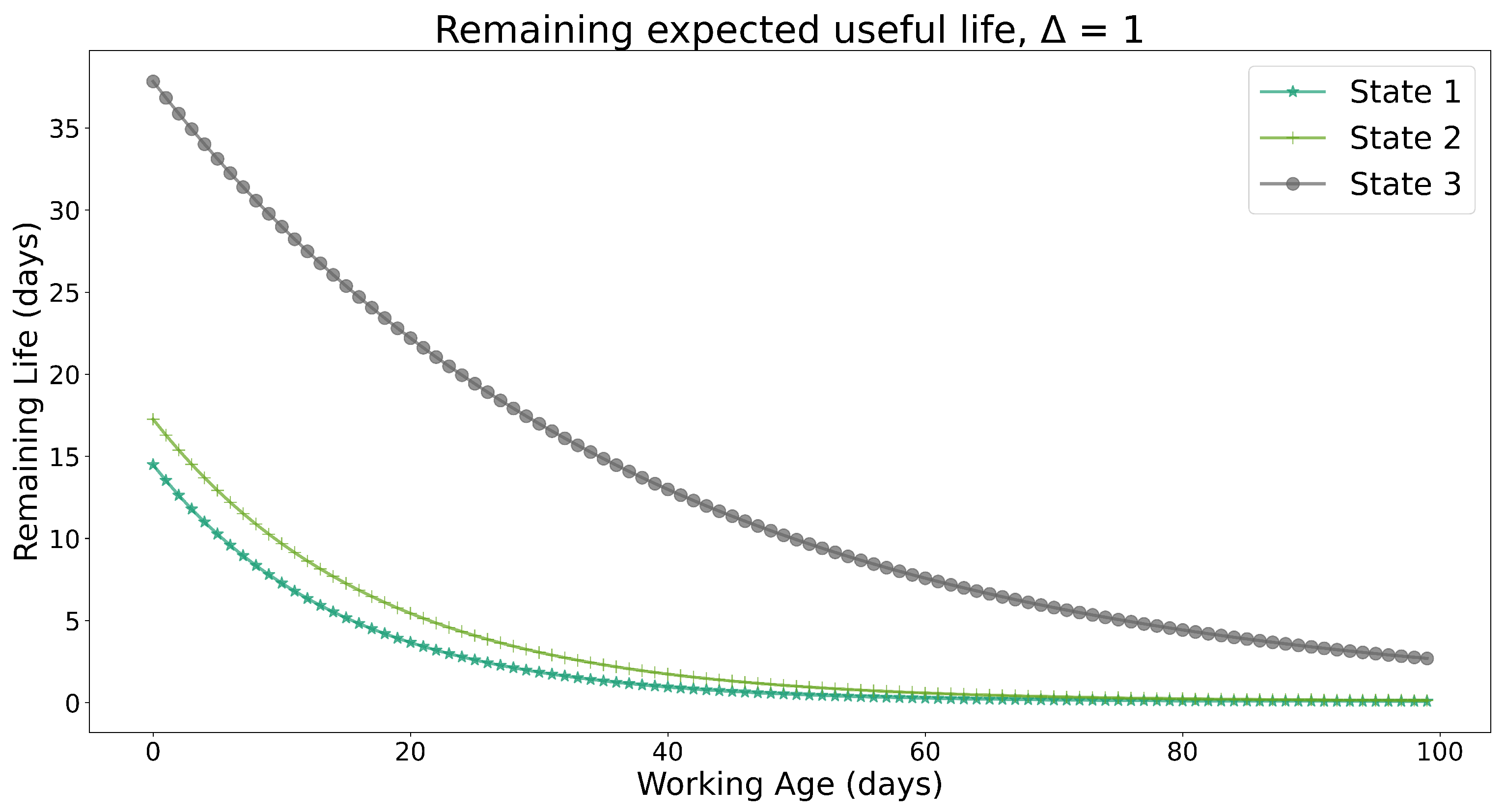
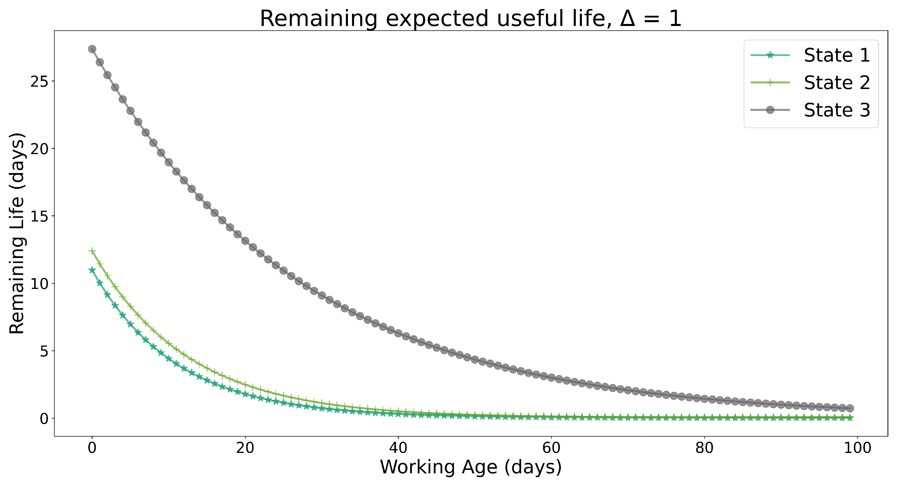
For predictive purposes and using the estimated conditional reliability functions as inputs, Figure 10 and Figure 11 show the remaining useful life (RUL) for the training and testing data, considering the evolution of the clustered covariate data throughout the states. It is observed that Cluster-State 3 can be regarded as the best condition, since its decay from the maximum RUL presents smooth behavior. On the other hand, State-1 is the worst clustered condition, since its decline was the most aggressive over the working age. Although this effect could be expected, the novelty of the present proposal remained as aforementioned. Namely, experienced knowledge input could be straightforward when separating band limits for one covariate, since it has only one measurement unit. Nevertheless, it is difficult for an expert to deliver a band-limit value when dealing with diverse covariates, especially when the combined measure unit does not represent a physical magnitude to evaluate directly. Hence, the proposed ML method complements expert knowledge under a novel condition assessment.

Figure 10.
Remaining useful life with training data.
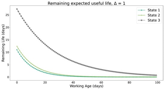
Figure 11.
Remaining useful life with testing data.
Now that the effect of the condition has been explained, the other component of the predictive PHM model (Equation (10)) is the contribution of age to the hazard rate. The values of and are all consequences of their interpretation in the conditional reliability and RUL from Figure 8, Figure 9, Figure 10 and Figure 11. All the values in Table 2 are higher than 1, indicating the wear-out stage in the asset life cycle. It means that the components under study were aging throughout the period. The characteristic life agrees with the values of the working age as well. However, it is interesting to note that in the earlier stage of the life cycle, the impact of the clustered condition was far more significant than the effect of age; that is, the difference in RUL across the states was more notorious. On the other hand, due to the PHM model, the RUL differences became shorter at the later stage of the asset life. This means that at elevated working ages, the effect of time is overcome because the overall condition of the asset is so degraded when reaching an advanced operating span.
Finally, the proposed ML condition assessment adds innovative knowledge about the clustered covariate process. Namely, it handles several vital signs with diverse sources and measurement units, thereby enabling a holistic approach. When implementing a predictive policy, this novel condition assessment allows a better understanding of the asset’s operational health to intervene at the exact moment (in contrast to a fixed-age replacement policy), thereby maximizing the assets’ RULs. It is demonstrated that this novel ML approach to address maintenance policies can provide significant results as an alternative or complement to the expert criterion, offering advantages, especially when dealing with more than one covariate, and ultimately increasing the expectation and precision of the remaining useful life for the critical assets.
5. Conclusions
This paper has introduced a model for defining the optimal covariate bands in condition assessment when dealing with PHM-CBM predictive maintenance decisions. A Machine Learning method has been provided to assess multiple asset conditions and complement expert knowledge, especially when the combined measure unit does not represent a physical magnitude that can be assessed directly. The results of this research do indeed lead to predictive maintenance decisions for different failure scenarios on different parameters, such as voltage and rotation, present in a variety of operational contexts. Using supervised classification and unsupervised clustering, this novel model sets the numbers of bands for the probability matrix and the optimal limits of each one, thereby strengthening the PHM model under realistic scenarios.
The cluster ranges for all covariates involved in the data under study are defined coherently and reliably. A proper transition matrix was obtained for both training and testing data. Afterward, the conditional reliability function was estimated for each cluster, thereby enhancing further CBM-predictive analyses. The procedure to conduct such an assessment has been developed.
We have demonstrated that this novel ML approach to address maintenance policies can provide significant results as an alternative or complement to the expert criterion, offering advantages, especially when dealing with more than one covariate, ultimately increasing the expectation and precision of the remaining useful life for the critical assets. As further work, there is an expectation of directly obtaining the transition probability matrices using GMM, an ML algorithm that allows for obtaining cluster membership probability surfaces. Finally, we built an enriched bridge between the decision areas of predictive maintenance strategy and Data Science.
Author Contributions
Conceptualization, D.R.G.; Methodology, D.R.G.; Validation, D.R.G. and V.Á.; Formal analysis, D.R.G., V.Á. and M.L.-C.; Writing—original draft preparation, D.R.G. and V.Á.; Writing—review and editing, D.R.G. and M.L.-C.; Supervision, D.R.G. All authors have read and agreed to the published version of the manuscript.
Funding
This research was supported by ANID through FONDECYT DE INICIACIÓN (Chile). Grant Numbers: 11190884 and 11180964.
Data Availability Statement
Not applicable.
Acknowledgments
The authors wish to acknowledge the financial support of this study by Agencia Nacional de Investigación y Desarrollo (ANID) through Fondo Nacional de Desarrollo Científico Y Tecnológico (FONDECYT) of the Chilean Government (Project FONDECYT INI 11190884 and Project FONDECYT INI 11180964).
Conflicts of Interest
The authors declare no conflict of interest.
References
- Safaei, N.; Jardine, A.K. Aircraft routing with generalized maintenance constraints. Omega 2018, 80, 111–122. [Google Scholar] [CrossRef]
- Nehring, M.; Knights, P.; Kizil, M.; Hay, E. A comparison of strategic mine planning approaches for in-pit crushing and conveying, and truck/shovel systems. Int. J. Min. Sci. Technol. 2018, 28, 205–214. [Google Scholar] [CrossRef]
- Godoy, D.R.; Pascual, R.; Knights, P. A decision-making framework to integrate maintenance contract conditions with critical spares management. Reliab. Eng. Syst. Saf. 2014, 131, 102–108. [Google Scholar] [CrossRef]
- Maletič, D.; Maletič, M.; Al-Najjar, B.; Gomišček, B. An analysis of physical asset management core practices and their influence on operational performance. Sustainability 2020, 12, 9097. [Google Scholar] [CrossRef]
- Galar, D.; Kans, M. The impact of maintenance 4.0 and big data analytics within strategic asset management. In Proceedings of the Maintenance Performance and Measurement and Management 2016 (MPMM 2016), Luleå, Sweden, 29–30 November 2017; pp. 96–104. [Google Scholar]
- Crespo, A.; Gómez, J.F.; Martínez-Galán, P.; Guillén, A. Maintenance management through intelligent asset management platforms (IAMP). Emerging factors, key impact areas and data models. Energies 2020, 13, 3762. [Google Scholar] [CrossRef]
- Jardine, A.K.; Lin, D.; Banjevic, D. A review on machinery diagnostics and prognostics implementing condition-based maintenance. Mech. Syst. Signal Process. 2006, 20, 1483–1510. [Google Scholar] [CrossRef]
- Azizi, F.; Salari, N. A novel condition-based maintenance framework for parallel manufacturing systems based on bivariate birth/birth–death processes. Reliab. Eng. Syst. Saf. 2023, 229, 108798. [Google Scholar] [CrossRef]
- Pedersen, T.I.; Vatn, J. Optimizing a condition-based maintenance policy by taking the preferences of a risk-averse decision maker into account. Reliab. Eng. Syst. Saf. 2022, 228, 108775. [Google Scholar] [CrossRef]
- Zheng, R.; Chen, B.; Gu, L. Condition-based maintenance with dynamic thresholds for a system using the proportional hazards model. Reliab. Eng. Syst. Saf. 2020, 204, 107123. [Google Scholar] [CrossRef]
- Cox, D.R. Regression models and life-tables. J. R. Stat. Soc. Ser. B (Methodol.) 1972, 34, 187–202. [Google Scholar] [CrossRef]
- Jardine, A.K.; Tsang, A.H. Maintenance, Replacement, and Reliability: Theory and Applications; CRC Press, Taylor & Francis Group: Boca Raton, FL, USA, 2005. [Google Scholar]
- Jardine, A.; Anderson, P.; Mann, D. Application of the Weibull proportional hazards model to aircraft and marine engine failure data. Qual. Reliab. Eng. Int. 1987, 3, 77–82. [Google Scholar] [CrossRef]
- Liu, H.; Makis, V. Cutting-tool reliability assessment in variable machining conditions. IEEE Trans. Reliab. 1996, 45, 573–581. [Google Scholar]
- Banjevic, D.; Jardine, A. Calculation of reliability function and remaining useful life for a Markov failure time process. IMA J. Manag. Math. 2006, 17, 115–130. [Google Scholar] [CrossRef]
- Mofolasayo, A.; Young, S.; Martínez, P.; Ahmad, R. How to adapt lean practices in SMEs to support Industry 4.0 in manufacturing. Procedia Comput. Sci. 2022, 200, 934–943. [Google Scholar] [CrossRef]
- Shinde, P.P.; Shah, S. A review of machine learning and deep learning applications. In Proceedings of the 2018 Fourth International Conference on Computing Communication Control and Automation (ICCUBEA), Pune, India, 16–18 August 2018; pp. 1–6. [Google Scholar]
- Rajendra, P.; Girisha, A.; Gunavardhana Naidu, T. Advancement of machine learning in materials science. Mater. Today Proc. 2022, 62, 5503–5507. [Google Scholar] [CrossRef]
- Sancho, A.; Ribeiro, J.; Reis, M.; Martins, F. Cluster analysis of crude oils with k-means based on their physicochemical properties. Comput. Chem. Eng. 2022, 157, 107633. [Google Scholar] [CrossRef]
- Li, T.; Rezaeipanah, A.; Tag El Din, E.M. An ensemble agglomerative hierarchical clustering algorithm based on clusters clustering technique and the novel similarity measurement. J. King Saud Univ. Comput. Inf. Sci. 2022, 34, 3828–3842. [Google Scholar] [CrossRef]
- Ezugwu, A.E.; Ikotun, A.M.; Oyelade, O.O.; Abualigah, L.; Agushaka, J.O.; Eke, C.I.; Akinyelu, A.A. A comprehensive survey of clustering algorithms: State-of-the-art machine learning applications, taxonomy, challenges, and future research prospects. Eng. Appl. Artif. Intell. 2022, 110, 104743. [Google Scholar] [CrossRef]
- Dhanachandra, N.; Manglem, K.; Chanu, Y.J. Image Segmentation Using K -means Clustering Algorithm and Subtractive Clustering Algorithm. Procedia Comput. Sci. 2015, 54, 764–771. [Google Scholar] [CrossRef]
- Lloyd, S. Least squares quantization in PCM. IEEE Trans. Inf. Theory 1982, 28, 129–137. [Google Scholar] [CrossRef]
- Forgy, E.W. Cluster analysis of multivariate data: Efficiency versus interpretability of classifications. Biometrics 1965, 21, 768–769. [Google Scholar]
- Kanungo, T.; Mount, D.M.; Netanyahu, N.S.; Piatko, C.D.; Silverman, R.; Wu, A.Y. An efficient k-means clustering algorithm: Analysis and implementation. IEEE Trans. Pattern Anal. Mach. Intell. 2002, 24, 881–892. [Google Scholar] [CrossRef]
- Chen, L.; Shan, W.; Liu, P. Identification of concrete aggregates using K-means clustering and level set method. Structures 2021, 34, 2069–2076. [Google Scholar] [CrossRef]
- El Ouadi, J.; Malhene, N.; Benhadou, S.; Medromi, H. Towards a machine-learning based approach for splitting cities in freight logistics context: Benchmarks of clustering and prediction models. Comput. Ind. Eng. 2022, 166, 107975. [Google Scholar] [CrossRef]
- Xu, H.; Ma, C.; Lian, J.; Xu, K.; Chaima, E. Urban flooding risk assessment based on an integrated k-means cluster algorithm and improved entropy weight method in the region of Haikou, China. J. Hydrol. 2018, 563, 975–986. [Google Scholar] [CrossRef]
- Troccoli, E.B.; Cerqueira, A.G.; Lemos, J.B.; Holz, M. K-means clustering using principal component analysis to automate label organization in multi-attribute seismic facies analysis. J. Appl. Geophys. 2022, 198, 104555. [Google Scholar] [CrossRef]
- Xinmin, G.; Zong’an, X.; Jun, Z.; Falong, H.; Jiangtao, L.; ZHANG, H.; Shuolong, W.; Shenyuan, N.; Ji’er, Z. An unsupervised clustering method for nuclear magnetic resonance transverse relaxation spectrums based on the Gaussian mixture model and its application. Pet. Explor. Dev. 2022, 49, 339–348. [Google Scholar]
- Huang, Y.; Englehart, K.B.; Hudgins, B.; Chan, A.D. A Gaussian mixture model based classification scheme for myoelectric control of powered upper limb prostheses. IEEE Trans. Biomed. Eng. 2005, 52, 1801–1811. [Google Scholar] [CrossRef]
- Reynolds, D.A. An overview of automatic speaker recognition technology. In Proceedings of the 2002 IEEE International Conference on Acoustics, Speech, and Signal Processing, Orlando, FL, USA, 13–17 May 2002; Volume 4, p. IV-4072. [Google Scholar]
- Hamdi, M.; Hilali-Jaghdam, I.; Elnaim, B.M.; Elhag, A.A. Forecasting and Classification of New Cases of Covid 19 before Vaccination Using Decision Trees and Gaussian Mixture Model. Alex. Eng. J. 2022, 62, 327–333. [Google Scholar] [CrossRef]
- Fahim, A. K and starting means for k-means algorithm. J. Comput. Sci. 2021, 55, 101445. [Google Scholar] [CrossRef]
- Steinley, D.; Brusco, M.J. Choosing the number of clusters in K-means clustering. Psychol. Methods 2011, 16, 285–297. [Google Scholar] [CrossRef]
- Habib, A.; Akram, M.; Kahraman, C. Minimum spanning tree hierarchical clustering algorithm: A new Pythagorean fuzzy similarity measure for the analysis of functional brain networks. Expert Syst. Appl. 2022, 201, 117016. [Google Scholar] [CrossRef]
- Lam, J.Y.J.; Banjevic, D. A myopic policy for optimal inspection scheduling for condition based maintenance. Reliab. Eng. Syst. Saf. 2015, 144, 1–11. [Google Scholar] [CrossRef]
- Yang, A.; Qiu, Q.; Zhu, M.; Cui, L.; Chen, W.; Chen, J. Condition based maintenance strategy for redundant systems with arbitrary structures using improved reinforcement learning. Reliab. Eng. Syst. Saf. 2022, 108643. [Google Scholar] [CrossRef]
- Azar, K.; Hajiakhondi-Meybodi, Z.; Naderkhani, F. Semi-supervised clustering-based method for fault diagnosis and prognosis: A case study. Reliab. Eng. Syst. Saf. 2022, 222, 108405. [Google Scholar] [CrossRef]
Disclaimer/Publisher’s Note: The statements, opinions and data contained in all publications are solely those of the individual author(s) and contributor(s) and not of MDPI and/or the editor(s). MDPI and/or the editor(s) disclaim responsibility for any injury to people or property resulting from any ideas, methods, instructions or products referred to in the content. |
© 2023 by the authors. Licensee MDPI, Basel, Switzerland. This article is an open access article distributed under the terms and conditions of the Creative Commons Attribution (CC BY) license (https://creativecommons.org/licenses/by/4.0/).

