Abstract
Solid rocket motors (SRMs) are widely used as propulsion devices in the aerospace industry. The SRM nozzle and combustion chamber are connected with a plugged-in structure, which makes it difficult to use the existing technology to investigate the internal conditions of the SRM during docking and assembly. The unknown deformation of the O-ring inside the groove caused by different assembly conditions will prevent the engine assembly quality from being accurately predicted. Algorithms such as machine learning can be used to fit mechanical simulation data to create a model that can be used to make predictions during assembly. In this paper, the prediction method uses the sampled parameters as boundary conditions and applies the finite element method (FEM) to calculate the stresses and strains of the O-ring under different assembly conditions. The simulation data are fitted using the gradient-enhanced Kriging (GEK) model, which is more suitable for high-dimensional data than the ordinary Kriging model. A genetic algorithm (GA) and conditional tabular generative adversarial networks (CTGAN) are used to optimize the prediction model and improve its accuracy as new data are incorporated. The proposed method is not only accurate but also efficient, allowing for a significant reduction in assembly time. The use of the surrogate model and FEM makes it possible to predict the stresses and strains of the O-ring in real-time, making the assembly process smoother and more efficient. In conclusion, the proposed method provides a promising solution to the challenges associated with the assembly process of SRM in the aerospace industry.
1. Introduction
SRM is widely used in missiles and various space products due to its simple design and high reliability, while seal failure is one of the main causes of accidents in SRM [1]. Under normal conditions, the contact pressure between the O-ring and the flange makes it difficult for high-pressure gas to escape [2]. However, if the O-ring breaks due to overstress, or if it is not compressed in place and fails to seal effectively, the resulting seal failure will result in a launch accident [3].
Due to the difficulty in detecting the interior of the SRM during the docking assembly process, it is challenging to test the seal quality of the SRM after assembly. Not only is the O-ring not visible during the assembly process (Figure 1), but more critically, any slight change in assembly position and orientation, irregular deformation of the thin-walled combustion chamber shell after filling, and tightening of the nozzle bolts will have a critical effect on the assembly stress distribution of the O-ring in a realistic assembly environment.
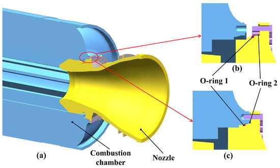
Figure 1.
Structure of the SRM: (a) Section view; (b) Before assembly; (c) After assembly.
In general, the prediction of seal life is usually performed by using failure mechanisms, by designing accelerated aging tests to predict the life of static seal structures, by predicting the reliability and life of O-rings based on room temperature degradation curves, or by using fracture mechanics combined with the finite element analysis to predict fatigue crack propagation failure [4,5,6]. Few studies have considered the assembly process of SRMs.
To evaluate whether an O-ring has failed or not, the FEM is typically used to calculate the stress and strain as the basis for failure determination. However, the FEM takes a long time to solve such non-linear problems, so it is not able to achieve a real-time prediction. Therefore, the current approach to such problems is still based on empirical judgments. The construction of a surrogate model that expresses such an assembly process will make the sealing level prediction easier. A predictive model of the seal condition is obtained by fitting the test data using machine learning [7,8]; most of the machine learning algorithms require a large number of samples, which is time-consuming for FEM. Kriging models are commonly used in digital twin modeling [9], failure probability estimation [10], finite element model updating [11], tooth face wear calculation [12], etc., which has the advantage of generating a more accurate surrogate model with fewer sample points.
In this paper, a Kriging model is proposed to represent the assembly result, in particular the sealing state. The FEM is used to simulate the stresses and strains of the O-ring under various assembly conditions, and a surrogate model is generated with the assembly condition parameters as input and the stresses or strains as output. The proposed model takes a new approach to machine learning, requiring fewer samples for training and optimizing performance using GAN and GA techniques. This results in a significant reduction in training time and resources while maintaining high accuracy. This surrogate model is used to predict the state of the SRM O-rings during assembly and to find the current optimal tightening sequence under these parameters.
2. Elastic–Plastic Model of Rubber O-Ring
The flange between the nozzle and the combustion chamber of the SRM is sealed by several rubber O-rings. As a nonlinear material, the elastic–plastic model of the rubber can be expressed by using the hyperelastic constitutive model. Mooney–Rivlin is one of the typical models that can more accurately approximate small strains within 150%, and the deformation of the SRM O-ring during assembly satisfies the small strain property. The strain energy density function for the 2 parameter Mooney–Rivlin model for rubber is as follows [13]:
where W is the strain energy density, and are the Rivlin coefficients, and are the 1st and 2nd Cauchy–Green deformation tensor invariants of the material, respectively, is the incompressibility of the material, J is the volume ratio ( for incompressible materials), is the principal elongation in 3 directions, and is the strain of the material.
The material parameters of the O-ring used in this study are listed in Table 1 and the stress–strain curve is shown in Figure 2.

Table 1.
Material parameters of the O-ring.
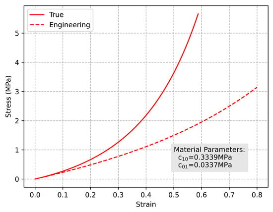
Figure 2.
Stress–strain curve of the O-ring.
Rubber, as an incompressible material, has a Poisson’s ratio and its Young’s modulus and shear modulus are related to the Mooney–Rivlin parameters as follows.
3. Assembly Simulation of the O-Ring
3.1. Assembly Condition Parameters
Assembly condition parameters are the basic boundary conditions for FEA. In the assembly process, different docking insertion angles and positions will affect the final sealing state. The flanges of each nozzle and combustion chamber also show irregular individual variations due to manufacturing errors, and different flange profiles result in different O-ring stresses. After assembly, different bolt tightening sequences on the flange will also result in different final stress distributions under the stress caused by the insertion.
The factors that affect the final stress distribution in the O-ring can be divided into three categories: position and orientation during assembly, manufacturing errors during processing, and bolt tightening sequence. (Figure 3).
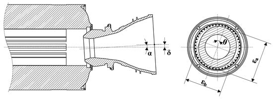
Figure 3.
Assembly condition parameters.
The combustion chamber and the nozzle are installed as follows: the combustion chamber is fixed and the nozzle is controlled by a parallel insertion platform, resulting in almost no nozzle rolling during the assembly process. Therefore, to simplify the model, only the pitch and yaw of the nozzle are considered as assembly orientation parameters, which can be transformed to a deflection angle instead , where indicates the yaw angle of the nozzle axis in the y-plane and indicates the pitch angle of the nozzle axis in the z-plane. In addition to orientation, the position of the nozzle in relation to the combustion chamber is also taken into account during insertion; and indicate the eccentric distance between the nozzle and the central axis of the combustion chamber in the y and z directions, respectively. The x-direction is not included in the parameters because it is the direction of the insertion.
Both will cause irregular flange deformation due to manufacturing errors and thin-walled chamber shells affected by gravity. The profile changes formed by deformation on the flange can be simplified to an elliptical shape, so the amount of deformation can be expressed in terms of relative ellipticity. is the relative ellipticity of the flange after deformation, and its expression is as follows:
where and are the maximum and minimum elliptical profile diameter deviations from the ideal profile diameter. and indicate the ellipticity of the nozzle and combustion chamber, respectively. and indicate the ellipticity of the two seal grooves. indicates the angle of the long axis of the elliptical profile with respect to the positive direction of the z-axis.
The nozzle periphery should also be tightened with a ring of bolts after docking to complete the SRM assembly. Residual bolt preload often changes due to the “elastic interaction” caused by the different sequence of bolt preload [14].
where is the initial bolt preload, is the final bolt preload, and is the elastic interaction matrix. The uneven residual preload of the bolts will cause different flange deformation, and the deformation of the flange will also affect the sealing performance of the SRM.
The deformation of the flange is directly related to the final preload force and is also influenced by the cross-sectional area -A, Young’s modulus E, and thickness h.
In the past, only a constant tightening sequence was used without considering the state of the nozzle after docking, which actually did not provide a better sealing effect. Thus, the prediction model will use the deflection angle, eccentric distance, and ellipticity to represent the condition parameters in the docking process, and the assembly process will be expressed as a tightening sequence after the docking. As shown in Figure 4, the upper right bolt is defined as bolt number 1, and the serial numbers are arranged clockwise. The tightening sequence is defined as an arrangement of tightened serial numbers. The SRM bolt assembly process is performed by one or two robots, either one bolt at a time or two bolts at a time. Under normal circumstances, two bolts tightened simultaneously is generally superior to a single bolt tightened at a time in terms of both efficiency and quality. However, to verify the advantages and disadvantages of the two tightening methods, two different cases are simulated separately in the following FEA.
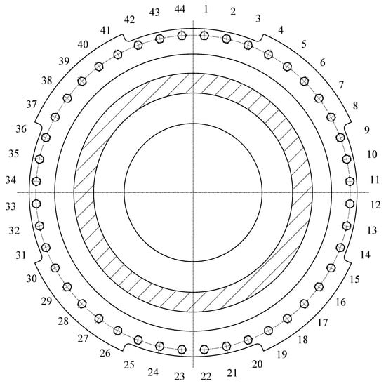
Figure 4.
Bolt serial number.
3.2. Selection of the Parameter Space
Theoretically, there are an infinite number of possible condition parameters in the design space, and it is not possible to calculate to calculate all assembly conditions when performing an FEA. This is because overusing data not only leads to problems such as overfitting, but is also impractical due to simulation time considerations. Therefore, the data are first sampled within the parameter limits prior to FEA, and the specific data sampled are selected for simulation.
Commonly used experimental design methods include the orthogonal design method, the design of experiments method, the crossover design method, the randomized block design method, the Monte Carlo method, the Latin hypercube sampling method (LHS), and so on. The results of sampling must ensure that the selected sample data can express the characteristics of the whole space without losing model features, and it is also not advisable to have too many redundant points, which will make the prediction model over-fit and affect the model accuracy. The LHS can represent global features with a small amount of data. It is superior to other sampling methods because it ensures that the sampled values can cover the entire distribution interval of the input random variables, making the sampled data more representative.
The LHS draws a total of n points from a p-dimensional space: first, each dimension is divided into non-overlapping intervals of equal probability, points are selected from the interval of each dimension, and then the selected points in each dimension are randomly combined in space. The deflection angle, eccentric distance, ellipticity, and bolt tightening order are sampled via the LHS. The number of samples must be greater than the dimension of the data model, and the sampled data points will be used in the subsequent simulation.
3.3. Finite Element Analysis of the O-Ring
After specifying the material parameters of the O-ring and defining the assembly condition parameters, an FEA of the SRM docking and bolt tightening process was performed. The 3D models of the combustion chamber, nozzle, O-ring, and bolt are created. In order to shorten the simulation period, the models are simplified and the parts of the models that are not involved in the simulation process or that have little effect on the simulation results are ignored. During the assembly process, the combustion chamber is completely fixed by the lift and bracket, and the movement of the nozzle is controlled by the 6-DOF parallel platform. During the docking process, the nozzle expansion section and the vector components, etc., have less influence on the O-ring, so only the nozzle flange and a small part of the nozzle throat are held. For the combustion chamber, the part of the tooling positioning bracket to the combustion chamber flange is retained because the thin-walled combustion chamber is more susceptible to gravity. Several typical assembly condition parameters are uniformly selected in the design domain and the docking assembly process of the SRM is simulated using ANSYS WORKBENCH 2022R1.
The contact settings for the simulation are as follows: (1) The inner edge of the combustion chamber flange and the outer edge of the nozzle flange are in frictional contact. (2) The outer surface of the combustion chamber flange and the end surface of the nozzle rabbet are in frictionless contact. (3) The smaller O-ring and the sealing groove surface are in rough contact. (4) The larger O-ring forms a rough contact with the surface and edge of the nozzle shoulder. (5) Two O-rings form a frictional contact with the inner surface and outer edge of the combustion chamber, respectively. (6) The bottom surface of the bolt head and the bottom surface of the nozzle bolt hole are in frictional contact. (7) The screw part of the bolt and the inner wall of the combustion chamber bolt hole are in no separation contact.
Since the seal, nozzle, and combustion chamber material parameters have been determined, the friction coefficient is also required for the simulation. The friction coefficient of the simulation has a large influence on the accuracy of the simulation results and is difficult to determine accurately due to the complexity of actual assembly conditions. Therefore, the friction coefficient was first approximated empirically based on the contact material, and then corrected based on the assembly test results of the test prototype (Figure 5). The friction coefficient between the nozzle and the combustion chamber was finally set at 0.11 and between the seal and the combustion chamber at 0.42.
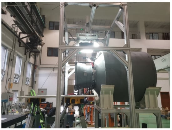
Figure 5.
Experimental prototype.
Nonlinear problems for finite element analysis include material nonlinearity, geometric nonlinearity, and boundary nonlinearity. The O-ring is installed in the nozzle sealing groove and shoulder; in the groove, the O-ring is sheared and squeezed during the assembly process, and it will gradually fill the bottom surface of the groove. Then, its boundary will change, which belongs to the boundary nonlinearity. The rubber of the O-ring is a hyperelastic material, which itself has material nonlinearity. Moreover, the hyperelastic material generates large strains and large displacements during extrusion, which are geometric nonlinearities. For the reasons mentioned above, the simulation is set up in a way to analyze nonlinear problems.
The simulation uses an enhanced Lagrangian contact algorithm with asymmetric contact behavior. Since the stiffness of the nozzle and combustion chamber is much higher than that of the O-ring, it is necessary to refine the mesh of the O-ring in order to analyze its deformation. The mesh size of the O-ring is set to 0.4 mm, a total of 13,473,181 nodes, 3,616,757 elements. The type of the element is SOLID 187. The mixed formulation and nonlinear mechanical element physics preference are used for the O-ring mesh. Fixed support is applied to the bottom of the nozzle and gravity constraints are applied to all geometry. The load step is divided into three stages: the first stage applies normal displacement to the O-ring to simulate the pre-compression process, the second stage applies displacement to the bottom of the combustion chamber to simulate the insertion process, and the third stage is the bolt tightening process.
Since the load is divided into three stages and the nonlinearity is stronger, the calculation does not converge easily. To ensure reliable analytical calculations and save the simulation cycles, a hybrid U-P element is adopted in the simulation setup to prevent the element volume from self-locking, while a nonlinear adaptive region mesh method is used, the large deformation switch is turned on, and restart analysis is used to help the calculation converge. The stresses on the O-ring under various parameters of the sampled conditions are simulated by FEA (Figure 6).

Figure 6.
FEA of the O-ring: (a) FEA with poor condition parameters and tightening sequences; (b) FEA with relatively ideal condition parameters and poor tightening sequences; (c) FEA with ideal condition parameters and tightening sequences.
Figure 7 compares the advantages and disadvantages of four different bolt tightening sequences under ideal conditions, and the points shown in the figure are the stress minimization tightening methods under the current element. As shown in Table 2, Pattern 4, i.e., the double-robots diagonally tightening method, is superior in most cases. Most of the elements in this method process lower stresses, which is consistent with empirical knowledge and previous studies [15]. Therefore, only double-robots tightening is considered for the bolt sequence FEA, which helps reduce the dimensionality of the surrogate model.
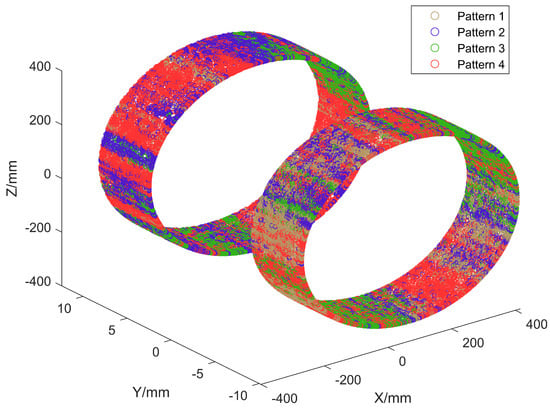
Figure 7.
Tightening pattern comparison.

Table 2.
Superiority percentage of tightening method.
4. Data Set Expansion Technology
Since nonlinear FEA is very time-consuming and difficult to converge, it is obviously impractical to simulate a large number of required samples, and the data expansion method can solve the problem of insufficient data volume at a lower time cost. Using Generative Adversarial Networks (GAN) [16], the original data distribution of the stress data set can be learned, expanded with data similar to the original data distribution as new data, and the original data distribution is used as a reference to extend the new data.
A GAN is composed of a generator G and a discriminator D. The generator forges data with the same distribution as the sample data by input noise, and the discriminator is used to distinguish the actual data from the forged data. Through the mutual game between the generator and the discriminator, the two optimize each other and continuously improve their own generative and discriminative abilities. Furthermore, finally, when the discriminator cannot discriminate the authenticity of the data generated by the generator, i.e., the generator and the discriminator reach Nash equilibrium, the data generated by the GAN can be considered equivalent to the actual data.
The generator and discriminator of GANs are composed of a Convolutional Neural Network (CNN). The random noise z is output as G(z) by the generator G, and the distribution of G(z) is as close as possible to the distribution of the actual sample p(x). The discriminator D needs to judge whether the generated data belongs to the distribution of the actual sample. If it matches the sample distribution, it outputs 1, otherwise it outputs 0 and make the generator to regenerate the data. Its objective function is [16]
where is the distribution of the actual sample data x, is the prior distribution of the noise z, and is the expectation.
However, traditional GANs are less capable and inefficient for learning multiple categories of data and are unable to generate category-specific data distributions. In contrast, the Conditional Generative Adversarial Networks (CGAN) can generate data from different categories. The objective function of a CGAN is as follows [17]:
The CGAN adds the label y as category constraint information to the GAN. The generator consists of noise z and labels y together as input, and the discriminator discriminates the similarity between the generated data and the real sample data x, and adjusts the generated data according to the label y.
Compared to CGAN, Tabular Generative Adversarial Networks (TGAN) [18] are more suitable for processing tabular data of all types, while Conditional Tabular Generative Adversarial Networks (CTGAN) [19] combine the CGAN with the TGAN to achieve processing of tabular data in the form of conditional classification. CTGAN is used to process the stress data set of O-rings for different assembly condition parameters. The generator of CTGAN consists of two fully connected layers and two deconvolutional layers, and its discriminator consists of two convolutional layers and two fully connected layers.
In Figure 8, the simulation results were expanded using CTGAN, and the data expansion results are shown below. The hollow points are the FEA data filtered by the LHS, and the solid points are the data expanded by the CTGAN.
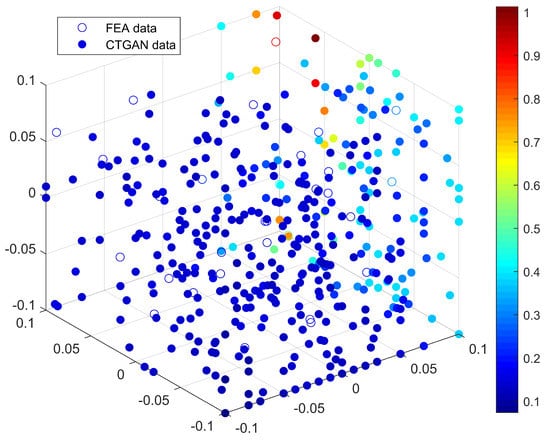
Figure 8.
Data expansion with CTGAN.
5. Kriging-Based Stress Prediction Model
5.1. Kriging Prediction Modeling
Kriging model [20] is a spatially self-covariance-optimal interpolation method that can use information from known points to unbiasedly estimate the response at unknown points. The main body of the Kriging model is based on the response surface method (RSM), but the advantage of the Kriging model over other surrogate models is that it does not require an excessive number of fitting parameters and samples. Kriging calculates the weights of the sample points under the constraint of minimum estimation variance, and linearly combines the sample points and weights to find the interpolated estimation of any point. Kriging has both local and global statistical properties due to the fact that it only uses data values in the vicinity of the estimation point rather than global data points in the prediction. However, Kriging is exponentially computationally expensive for high-dimensional data, which makes ordinary Kriging unsuitable for training in high-dimensional parameter spaces. The solution to this problem is to introduce gradient information [21]. Gradient-enhanced Kriging (GEK) incorporates gradient information into the structure of the Kriging model, which helps improve the accuracy of the Kriging model and allows the use of less data [22,23,24].
The specific methodological process of stress and strain modeling is identical, and only the stress prediction modeling process is described below. The simulation result was selected as the initial input for the surrogate model: eccentricity distance, deflection angle, ellipticity, and bolt tightening sequence were used as input variables, and stress (strain) values were used as output results.
The theoretical model of Kriging is composed of a regressive part and a stochastic part together [20]:
where the former term corresponds to the regressive part of the RSM, which generally can also be multiplied by a polynomial function to provide the overall approximate expectation of the Kriging model, and the latter term is the stochastic part. is the unknown regression coefficient; z(x) is the random error function and its mean , variance , the covariance of two data points , where is the spatial correlation equation.
where Y is the response value in the sample data set, R is the correlation matrix between sample points composed of correlation functions, r is the correlation vector composed of correlation functions, and .
GEK adds gradient information to Kriging, and for the m-dimensional n-sample points problem, the sampled data and response values of the input sample data set can be expressed as follows:
where is the element in the lower half of matrix X, , and denote the sample points providing partial derivatives for the jth sample of the kth dimension, and denotes the partial derivative of the jth response for the kth dimension sample.
The GEK theoretical model is the same as the ordinary Kriging (Formula (11)), whose random error function satisfies , and the covariance satisfies
where . Spatial correlation equations can generally be used, such as the Gaussian correlation equation:
where is the correlation parameter.
The response expression for GEK can be derived using the unbiased condition combined with the Lagrange multiplier method [25]:
where , the GEK correlation matrix , and the GEK correlation vector are as follows:
The correlation matrix R is composed of correlation functions:
The correlation vector r is also composed of correlation functions.
The predicted mean squared deviation of the estimated response from the GEK model is
The assembly condition parameters combined with the bolt tightening sequence are used as the input of the GEK model, and the simulation result data are used as the output to generate the original GEK model.
5.2. Optimization of the GEK Model
Since the sample points are under a uniform distribution, but the stress distribution under the assembly state design space is not uniform, this leads to the fact that the original GEK model accuracy may not be sufficient. When the accuracy of the model is inadequate, the judgment of the prediction model will have errors, causing the loss of local features of the model.
For this purpose, it is necessary to increase the density of sample points where the model error is significant. The MSE provided by the GEK model can be used as a reference for accuracy evaluation, and the Genetic Algorithm (GA) can be used to search for the maximum value of it. The data generated by CTGAN are selected from those with the closest spatial location and added to the GEK model to improve its accuracy.
In the above formula, and are the upper and lower limits of the design variables, is the set of design variables, is the assembly parameter, and is the bolt tightening sequence.
After adding the new data, the model is reconstructed and the accuracy of the model is evaluated again. In this way, new data are added to the model using GA and CTGAN to iteratively update the model until the accuracy of the model is sufficient to achieve the purpose of accurate prediction.
Figure 9 briefly illustrates the effect of several assembly condition parameters on the stress distribution at a single element of the O-ring when other assembly condition parameters are held constant. Figure 9a,b shows the effect of deflection angle and eccentric distance on stress, while Figure 9c–e shows the effect of ellipticity. The figure shows that a single assembly condition parameter can lead to high local element stress. The superimposed effect of multiple poor parameters leads to stress concentration in the O-ring, resulting in damage.
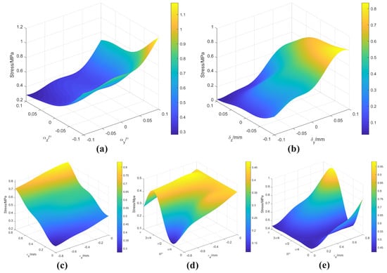
Figure 9.
Kriging model of single element: (a) Effect of the deflection angle; (b) Effect of the eccentric distance; (c) Effect of the maximum and minimum elliptical diameter; (d) Effect of the maximum elliptical diameter and elliptical angle; (e) Effect of the minimum elliptical diameter and elliptical angle.
Each element has its own independent GEK model, and all GEK models together form a model set: the digital twin prediction model for the SRM O-ring. Figure 10 shows a test of the predictive capability of the GEK model, using a portion of the FEA results not included in the model as a test set to verify that the predictions of the GEK model match the simulation results. The cross-validation results show that the accuracy of this prediction model is basically stable within 3%, which indicates that the model can accurately predict the stress values and locations during the SRM assembly process.
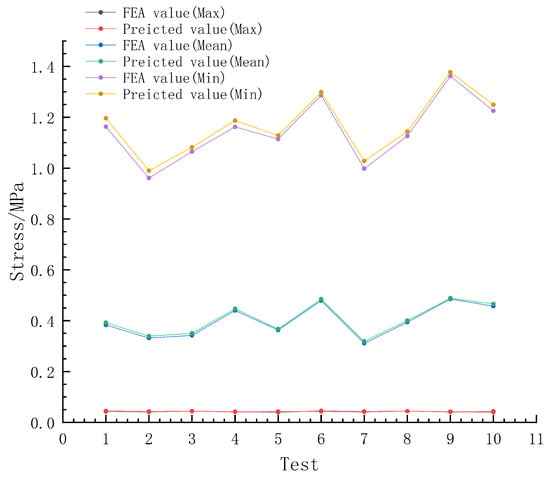
Figure 10.
Cross validation.
6. Prediction Process
During the docking assembly process, the nozzle is assembled by a 6-DOF parallel platform with a series of force–position sensors that provide real-time assembly position and orientation signals. The point cloud data of the flange is captured by a 3D laser scanner to obtain the ellipticity of the flange with simplified shape data.
With the assembly position, orientation, and ellipticity as input, the data are transferred in real-time to the prediction model, which searches for predicted values within seconds and generates a real-time nephogram of the current moment, with the maximum stress location and value displayed. At the same time, the model will also find the optimal bolt tightening sequence for the current assembly condition according to the principle of minimum average stress, which is achieved by GA:
where is the assembly parameter in the current assembly condition.
To improve the reliability of the model, and to account for the inevitable errors in the prediction model, a warning is given when the predicted maximum stress reaches 90% of the design allowable stress value. In this way, the purpose of guiding the assembly process can be achieved. The entire prediction workflow is shown in in Figure 11.
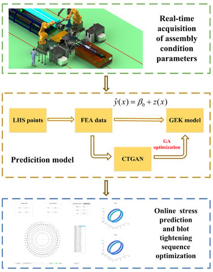
Figure 11.
Workflow of the prediction model.
7. Conclusions
This paper demonstrates the applicability of combining the FEM and surrogate model for predicting assembly stresses and strains in real-time. By utilizing this innovative technique, this method can replace time-consuming simulations and primitive trial assemblies, significantly reducing the assembly time from several days to just a few hours, which leads to a remarkable improvement in assembly efficiency.
In contrast to the traditional neural network model and Kriging model, using the GEK model, which is better suited for small samples and high-dimensional variables, is more advantageous in terms of efficiency and fitting of high-dimensional data. The prediction model’s optimization is another key aspect of this study, which significantly improves the accuracy of the model. It can not only achieve online prediction during the assembly process to make an accurate judgment on whether the O-ring will fail during the assembly process, but also provide the optimal tightening sequence under the current assembly condition based on the principle of minimum stress, which is more reliable than a fixed sequence. However, the use of simplified 3D models might cause errors in the simulation, leading to slight deviations in the current prediction results. Further improvements to the prediction model are needed in the future, such as using a complex point cloud shape model and more efficient algorithms. These modifications will ultimately enhance the accuracy and efficiency of the prediction model.
Author Contributions
Conceptualization, J.Z.; methodology, J.Z.; software, J.Z.; validation, J.Z.; formal analysis, J.Z.; writing—original draft preparation, J.Z., Y.W., J.W., R.C. and Z.X.; writing—review and editing, J.Z. All authors have read and agreed to the published version of the manuscript.
Funding
This research was funded by the National Key Research and Development Program of China (No. 2022YFB3306000), Independent project of the State Key Laboratory of Robotics (No. 2023-Z17).
Data Availability Statement
Not applicable.
Acknowledgments
The authors are grateful for the support from the National Key Research and Development Program of China (No. 2022YFB3306000), Independent project of the State Key Laboratory of Robotics (No. 2023-Z17). The authors are grateful to other participants of the project for their cooperation.
Conflicts of Interest
The authors declare that there are no conflicts of interest regarding the publication of this paper.
Abbreviations
The following abbreviations are used in this paper:
| SRM | Solid rocket motor |
| FEM | Finite element method |
| FEA | Finite element analysis |
| LHS | Latin hypercube sampling |
| GAN | Generative adversarial networks |
| CTGAN | Conditional tabular generative adversarial networks |
| RSM | Response surface method |
| GEK | Gradient-enhanced Kriging |
| MSE | Mean squared error |
| DOF | Degree of freedom |
| GA | Genetic algorithm |
References
- Dalal, S.R.; Fowlkes, E.B.; Hoadley, B. Risk analysis of the space shuttle: Pre-Challenger prediction of failure. J. Am. Stat. Assoc. 1989, 84, 945–957. [Google Scholar] [CrossRef]
- Sivakumar, V.; Palaninathan, R. FE analysis of contact pressure prediction on O-rings used in solid rocket booster segment joints. Int. J. Sci. Eng. Appl. 2012, 1, 8–16. [Google Scholar] [CrossRef]
- Jingdong, L.; Lipei, H. Research on recognition algorithm of seal fitting point based on compressibility control. In Proceedings of the 2017 29th Chinese Control And Decision Conference (CCDC), Chongqing, China, 28–30 May 2017; pp. 6259–6264. [Google Scholar]
- Shao, Y.; Kang, R. A life prediction method for O-ring static seal structure based on Physics of Failure. In Proceedings of the 2014 Prognostics and System Health Management Conference (PHM-2014 Hunan), Zhangiiajie, China, 24–27 August 2014; pp. 16–21. [Google Scholar]
- Sun, L.; Gu, X.; Feng, L.; Di, Y. Reliability analysis of rubber O-rings used in the rockets. In Proceedings of the 2016 IEEE International Conference on Industrial Engineering and Engineering Management (IEEM), Bali, Indonesia, 4–7 December 2016; pp. 1392–1396. [Google Scholar]
- Zine, A.; Benseddiq, N.; Abdelaziz, M.N. Rubber fatigue life under multiaxial loading: Numerical and experimental investigations. Int. J. Fatigue 2011, 33, 1360–1368. [Google Scholar] [CrossRef]
- Choi, J.; Quagliato, L.; Lee, S.; Shin, J.; Kim, N. Multiaxial fatigue life prediction of polychloroprene rubber (CR) reinforced with tungsten nano-particles based on semi-empirical and machine learning models. Int. J. Fatigue 2021, 145, 106136. [Google Scholar] [CrossRef]
- He, G.; Zhao, Y.; Yan, C. Application of tabular data synthesis using generative adversarial networks on machine learning-based multiaxial fatigue life prediction. Int. J. Press. Vessel. Pip. 2022, 199, 104779. [Google Scholar] [CrossRef]
- Bárkányi, Á.; Chovan, T.; Nemeth, S.; Abonyi, J. Modelling for digital twins—potential role of surrogate models. Processes 2021, 9, 476. [Google Scholar] [CrossRef]
- Cao, R.; Sun, Z.; Wang, J.; Guo, F. A single-loop reliability analysis strategy for time-dependent problems with small failure probability. Reliab. Eng. Syst. Saf. 2022, 219, 108230. [Google Scholar] [CrossRef]
- Zhu, Q.; Han, Q.; Liu, J.; Yu, C. High-Accuracy Finite Element Model Updating a Framed Structure Based on Response Surface Method and Partition Modification. Aerospace 2023, 10, 79. [Google Scholar] [CrossRef]
- Dong, K.; Sun, Z. Application of Kriging Model to Gear Wear Calculation under Mixed Elastohydrodynamic Lubrication. Machines 2022, 10, 490. [Google Scholar] [CrossRef]
- Kim, B.; Lee, S.B.; Lee, J.; Cho, S.; Park, H.; Yeom, S.; Park, S.H. A comparison among Neo-Hookean model, Mooney-Rivlin model, and Ogden model for chloroprene rubber. Int. J. Precis. Eng. Manuf. 2012, 13, 759–764. [Google Scholar] [CrossRef]
- Bibel, G.D.; Ezell, R.M. An Improved Flange Bolt-Up Procedure Using Experimentally Determined Elastic Interaction Coefficients. J. Press. Vessel Technol. 1992, 114, 439–443. [Google Scholar] [CrossRef]
- Wang, Y.; Liu, Y.; Wang, J.; Zhang, J.; Zhu, X.; Xu, Z. Research on Process Planning Method of Aerospace Engine Bolt Tightening Based on Digital Twin. Machines 2022, 10, 1048. [Google Scholar] [CrossRef]
- Goodfellow, I.; Pouget-Abadie, J.; Mirza, M.; Xu, B.; Warde-Farley, D.; Ozair, S.; Courville, A.; Bengio, Y. Generative adversarial networks. Commun. ACM 2020, 63, 139–144. [Google Scholar] [CrossRef]
- Mirza, M.; Osindero, S. Conditional generative adversarial nets. arXiv 2014, arXiv:1411.1784. [Google Scholar]
- Xu, L.; Veeramachaneni, K. Synthesizing tabular data using generative adversarial networks. arXiv 2018, arXiv:1811.11264. [Google Scholar]
- Xu, L.; Skoularidou, M.; Cuesta-Infante, A.; Veeramachaneni, K. Modeling tabular data using conditional gan. Adv. Neural Inf. Process. Syst. 2019, 32. [Google Scholar]
- Krige, D.G. A statistical approach to some basic mine valuation problems on the Witwatersrand. J. South. Afr. Inst. Min. Metall. 1951, 52, 119–139. [Google Scholar]
- Ulaganathan, S.; Couckuyt, I.; Dhaene, T.; Degroote, J.; Laermans, E. High dimensional Kriging metamodelling utilising gradient information. Appl. Math. Model. 2016, 40, 5256–5270. [Google Scholar] [CrossRef]
- Han, Z.H.; Görtz, S.; Zimmermann, R. Improving variable-fidelity surrogate modeling via gradient-enhanced kriging and a generalized hybrid bridge function. Aerosp. Sci. Technol. 2013, 25, 177–189. [Google Scholar] [CrossRef]
- Chung, H.S.; Alonso, J. Design of a low-boom supersonic business jet using cokriging approximation models. In Proceedings of the 9th AIAA/ISSMO Symposium on Multidisciplinary Analysis and Optimization, Atlanta, GA, USA, 4–6 September 2002; p. 5598. [Google Scholar]
- Chung, H.S.; Alonso, J. Using gradients to construct cokriging approximation models for high-dimensional design optimization problems. In Proceedings of the 40th AIAA Aerospace Sciences Meeting & Exhibit, Reno, NV, USA, 14–17 January 2002; p. 317. [Google Scholar]
- Sacks, J.; Welch, W.J.; Mitchell, T.J.; Wynn, H.P. Design and analysis of computer experiments. Stat. Sci. 1989, 4, 409–423. [Google Scholar] [CrossRef]
Disclaimer/Publisher’s Note: The statements, opinions and data contained in all publications are solely those of the individual author(s) and contributor(s) and not of MDPI and/or the editor(s). MDPI and/or the editor(s) disclaim responsibility for any injury to people or property resulting from any ideas, methods, instructions or products referred to in the content. |
© 2023 by the authors. Licensee MDPI, Basel, Switzerland. This article is an open access article distributed under the terms and conditions of the Creative Commons Attribution (CC BY) license (https://creativecommons.org/licenses/by/4.0/).