Abstract
Industrial actuator systems play an important role in mechanical manufacture, chemical production and other industrial processes. There is important theoretical research significance and engineering application value in accurately modeling and accurately controlling for an industrial actuator system with dead-zone input nonlinearity. The structure and order of the system are determined by the mechanism relationship of the system. Based on sampled data, an identification algorithm is proposed to describe the main dynamic characteristics of the system output. The convergence property of the proposed identification algorithm is also analyzed. Process faults may reduce the tracking control accuracy of the industrial actuator system. By using an intermediate observer to estimate the faults, a fault-tolerant synchronous control feedback rate is designed to compensate faults. The input dead-zone block may weaken the feedback control performance of the input signal and reduce the control precision. According to the dead-zone input nonlinearity model parameter, a compensator is introduced to transform the dead-zone function into a linear function passing through the origin of coordinates. The transformed and dynamic linear segment of the system constitute the generalized linear system. The model predictive control (MPC) strategy is designed to achieve robust and precise control by eliminating the effects of measurement noise. The results of numerical simulation and experimental test verify the superiority and merit of the modeling and fault-tolerant control strategy. The research results of this paper can provide a good reference and guidance for other complex systems in theoretical research and engineering applications.
1. Introduction
With the development of the manufacturing industry, higher requirements are put forward for the control accuracy and safe operation of industrial actuator systems [1,2,3]. The establishment of an accurate industrial system model is necessary for implementing process control and safety monitoring [4]. Using the mechanism analysis method and data-driven method, the establishing dynamic model of industrial system has important theoretical research significance and engineering application value [5]. The model-based controller design is easy to implement and has high control precision.
The industrial actuator system may work in a stable state, integral state, nonlinear state, or closed-loop state [6]. Therefore, it is necessary to select an appropriate modeling scheme according to the structure and working mode of the industrial actuator system. The modeling methods for industrial actuator systems are mainly divided into mechanism modeling method, data-driven modeling method, and hybrid modeling method [7]. The mechanism modeling method describes various characteristics of the process, and has strong explanatory and adaptability capacity for the specific process [8]. Due to the complexity of the process, it is difficult for the mechanism model to accurately describe all the characteristics of the process and the complex relationship between variables [9]. The prediction accuracy of the mechanism model is usually not high. The mechanism model usually involves complex calculus operations and a large number of undetermined parameters, which reduces its convenience in application [10]. The data-driven modeling method fully mines the data information related to the process and has the advantages of simple theory and easy implementation [11]. The internal mechanism relationship of the industrial system has strong coupling characteristics, and the data-driven modeling scheme is suitable for selection. By analyzing the mechanism of system, the model structure and order can be determined [12]. The data-driven identification method can obtain the main dynamic characteristics of the industrial system [13]. Therefore, this paper will study the data-driven modeling of industrial actuator system based on the sampled data.
Data-driven modeling of industrial systems is a hot topic for researchers. A series of scientific research achievements have been obtained [14]. By analyzing experiment data, the choke finger system is modeled by a block-oriented model with a nonlinear dynamic input. A recursive algorithm has been proposed to estimate the model parameters [15]. A two-stage identification method for Hammerstein systems, including not necessarily symmetric preload and dead-zone nonlinearity, has been developed and involves least-squares-like estimators and periodic input signals, which guarantee the consistency of all estimators [16]. By combining a data assignment and parameter estimation technique, a hybrid system consisting of a Piecewise Auto-Regressive eXogeneous (PWARX) structure has been developed for a rainfall-runoff system [17]. By designing sufficient excitation signals to persistently excite industrial Hammerstein–Wiener systems with dead-zone input nonlinearity, the main dynamic characteristics of the system can be obtained based on the least-squares estimation strategy [18]. A one-step adaptive parameter estimation framework has been presented for identification of asymmetric dead-zone parameters in sandwich systems. A continuous piecewise linear neural network and an adaptive observer are designed to avoid using intermediate variables [19]. These modeling strategies provide a guidance for data-driven modeling of industrial systems with dead-zone input nonlinearity.
Inevitable faults and random disturbances may affect the product quality and control accuracy of industrial operating systems. The research of disturbance rejection control based on the model has important engineering significance and theoretical research value [20]. Some important achievements have been made in fault-tolerant control and model predictive control. For outage faults and loss-of-effectiveness faults, a distributed adaptive fault-tolerant controller based on finite-time observer is designed to solve the cooperative output regulation problem, in which the solvability of the regulator equations is also guaranteed [21]. A broad learning system (BLS)-based adaptive full-state constrained controller has been investigated for a class of space unmanned systems (SUSs) subjected to the actuator faults and input nonlinearities. By estimating the lower boundary of the nonlinear actuator effectiveness, the unstable dynamic caused by the actuator faults and input nonlinearities can be overcome [22]. Based on the stable kernel representation, data-driven realization and design of feed-forward fault-tolerant control systems with embedded residual generation have been studied in the literature [23]. An adaptive fault-tolerant control design has been proposed for a flexible Timoshenko arm considering the effects of actuator failures, backlash-like hysteresis, and external disturbances [24]. The input dead-zone block can weaken the exciting characteristics of the control signal and limit the amplitude of the control signal. Based on the identification model, the MPC strategy can better achieve accurate control. By substituting event-triggered law for the receding horizon principle in predictive control, an event-triggered closed-loop subspace predictive control algorithm has been proposed for linear discrete-time systems with an unknown plant model [25]. A combined MPC and deep reinforcement learning solution has been presented, which can minimize stopping of trams at intersections while reducing delay of general vehicles [26]. A weighted-coupling CSTR (WCCSTR) model has been developed for the goethite process by introducing weighted parameters, and an MPC scheme has been designed to achieve the process performance goals and minimize the process cost [27]. A multi-objective model predictive control (MO-MPC) of constrained nonlinear systems has been proposed and the optimal solutions are obtained by solving a hierarchy of single objective optimization problems [28]. For the control system with actuator saturation and dead-zone nonlinearity, two different control strategies based on MPC have been implemented. One relies on hybrid MPC, and the other is based on dead-zone inversion and standard MPC [29]. A dead-zone compensating control law and a recursive estimator have been derived for Hammerstein systems with symmetric dead-zone input non-linearity and colored noise [30]. This paper presents a model-based strategy for fault tolerance in non-linear chemical processes. An observer-based fault detection and diagnosis scheme has been implemented to compensate the effects induced by actuator and sensor faults [31]. By employing some transformations, a part of the unknown dead-zone and external disturbance are regarded as a composite disturbance. An adaptive fault-tolerant boundary control has been developed by utilizing strict formula derivations to compensate for unknown composite disturbance, dead-zone, and actuator fault in the flexible string system [32]. By using fault detection and isolation technology, an active fault-tolerant model predictive control strategy with a hierarchal structural design is developed for a direct methanol fuel cell (DMFC) system with fault [33]. The controller design based on the established model can not only improve the control performance of linear time invariant systems but also improve the control precision of linear parameter-varying (LPV) systems. Switched gain-scheduling LPV controllers with fault-tolerance have been designed for engine exhaust gas recirculation (EGR) valve system with nonlinear dry friction [34]. The results of the existing literature in different fields can provide good guidance and reference for the research of this paper [35]. Based on the established nonlinear input dead-zone system model, the combination of fault-tolerant control technology and MPC technology can effectively eliminate the influence of dead-zones and disturbance.
In this paper, the theory of data-driven modeling and the scheme of fault-tolerant model predictive control are studied for industrial actuator systems with dead-zone input nonlinearity. A typical nonlinear industrial control system is introduced and designed. The structure and model order of the system are determined by mechanism analysis technique. The system is described by a nonlinear Hammerstein block system. The system model is established by a data-driven identification method. The parametric identification model can describe the main dynamic characteristics of the system. An intermediate observer is used to estimate the process faults signal. A fault-tolerant synchronous control feedback rate based on fault estimation is designed to compensate faults. In order to eliminate the weakening effect of dead-zone on control signal, a compensator has been introduced to transform the dead-zone function into a linear function. The MPC strategy was designed for the generalized linear system to achieve precise control. By comparing with the existing method, the effectiveness of the proposed modeling algorithm and control strategy will be cross-verified by using the numerical example and experimental platform. The rest of this paper is organized as below. A typical networked industrial control system will be introduced and designed in Section 2. Section 3 includes a system mechanism analysis and modeling problem description. The system data-driven identification algorithm and convergence analysis will be given in Section 4. The fault-tolerant model predictive control method will be presented in Section 5. The numerical simulation and experiment test are presented in Section 6. Finally, some main conclusions are drawn in Section 7.
2. Industrial Control System
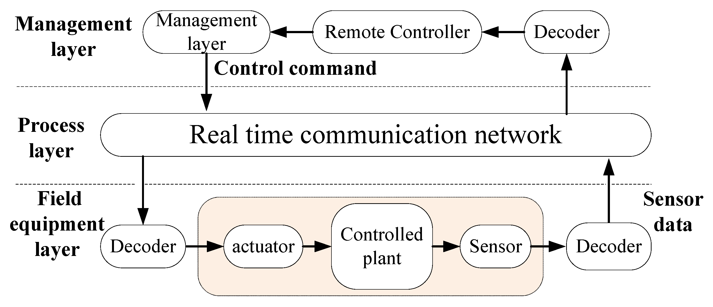
An industrial actuator control system is constructed on the basis of a real-time communication network and is mainly composed of a management layer, process layer, and field equipment layer, as shown in Figure 1. The management layer is a comprehensive information processing and human–computer interaction center, which is used to realize data monitoring, data storage, data management, and remote settings. The process layer is the core link for connecting the management layer and the field equipment layer, which is mainly used to collect sensor data of the field equipment layer and deliver management control instructions. The field equipment layer mainly includes actuators, controlled objects, and sensors. The remote controller and field device layers are located in different physical spaces and interact with each other through real-time communication networks. The typical industrial actuator control experimental system is constructed as shown in Figure 2.
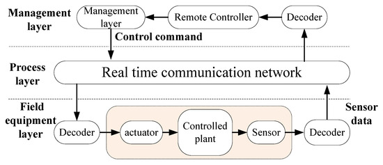
Figure 1.
Structure diagram of networked industrial system.
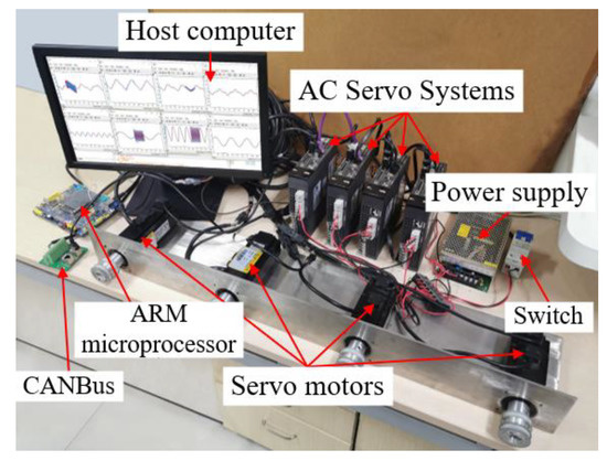
Figure 2.
Industrial control system platform.
The main functional modules involved in the system include network communication function, reset function, controlled mode function, desired trajectory function, start and stop function, and state monitoring function. The PC communicates with the embedded interface board by using the general Ethernet TCP/IP protocol. The data interaction between embedded interface board and servo driver is realized by CANopen protocol. The design based on PyQt5 and Qt Designer framework can provide an API interface and human–computer interaction interface with graphical editing function. The upper computer software implements data processing. The embedded interface board receives the working condition information uploaded from the onsite device and sends it to the PC via the Ethernet. The PC calculates the control quantity via the controller and sends it to the embedded interface board. After the embedded interface board’s parses and transforms, the closed-loop control of the system can be realized. The detailed parameter configuration of the experimental platform is shown in Table 1.

Table 1.
Parameter configuration of platform.
3. Modeling Problem Description
When the servo driver works in torque mode, the uniaxial servo system satisfies the torque balance equation
where is the electromagnetic torque; is the no-load torque caused by cogging torque and friction between the shaft and the bearing; is the angular velocity of the motor; is the friction coefficient; is the inertia of the uniaxial servo system in torque mode.
For motion control systems, no-load torque is usually used as a fixed servo parameter. When the driving torque is less than the no-load torque, the motion system cannot be driven, and the system presents the phenomenon of low input cutoff. With the aging of the motor and inter-shaft wear, the no-load torque in different rotation directions often changes slightly. Therefore, the no-load torque of the motor in different rotation directions is defined as two unequal constants and . According to Equation (1), the discrete time model of the uniaxial servo system under the torque model can be described as
where is the intermediate variable.
where and are the line segment slopes of the nonlinear input function.
Mechanism analysis can determine the model structure and parameters to be estimated by using electromagnetic theory. However, electromagnetic torque, no-load torque, angular velocity, friction coefficient, and moment of inertia of the motor cannot be determined and predicted by experimental tests. The parameters in the equipment manual are ideal values under certain assumption conditions, which are not complete and cannot reflect the dynamic operating characteristics of the system. Therefore, the dynamic model of the system can be established by using data-driven technology.
4. Parametric Identification Algorithm
4.1. Identification Algorithm
For industrial actuator systems with dead-zone input nonlinearity, the nonlinear Hammerstein structural model can be used to fit the system output. Without adding additional test sensors, the Hammerstein model can use the input and output data to realize the decoupled identification of the linear and nonlinear parts of the system. The Hammerstein model uses a combination of static nonlinear block and linear dynamic block to describe the system. Its system structure is shown in Figure 3.

Figure 3.
Hammerstein structure with dead-zone input nonlinearity.
The nonlinear system can be described as
where is the measurable input excitation signal; is an unmeasured intermediate signal; is the output response signal; is a Gaussian white noise signal with zero mean and variance ; is the backward shift operator.
The polynomials and are coprime and defined as follows
where and are the order of the system. Note that for unknown system dynamics, the model order is increased one by one, and their output prediction errors are also computed. The optimal model order may be determined by using the Akaike information criterion or a hypothesis testing condition [18].
The output function of the static nonlinear block is expressed as follows
The Equation (7) can be expressed as follows
where is an indicator function and defined as
Assuming that the system satisfies the zero initial condition, i.e., , , for . The system operates in open loop conditions, i.e., is uncorrelated with . The purpose of identification is to use sampled data to determine unknown model parameters.
Define the following vector
Combining Equations (10)–(15), the Equation (8) can be rewritten as
Combining Equations (4)–(6) and (16), the model output can be expressed as
The parameter and information vector expressions are, respectively, defined as follows
where .
Equation (17) can be rewritten as
The prediction output error is defined as
The estimation problem of the parameter vector is essentially the problem of minimizing the output error cost function.
where
The dead-zone parameters and can be calculated from the estimated values of the parameter vector, i.e.,
The established recursive least-squares algorithm for estimating is summarized as follows
By setting , a unique dead-zone parameter vector can be obtained. The parameter vector is represented as
4.2. Convergence Characteristic of Identification Algorithm
In this section, the convergence error of the proposed identification algorithm will be analyzed. Define parameter estimation error by
From Equations (26) and (27), we can obtain
Since the gain vector satisfies . By substituting Equation (20) into (32), yields
where
Due to
Multiplying both sides of Equation (34) by , we have
Substituting Equation (35) into Equation (33), can be expressed as
where , , and .
Through the above analysis, it can be seen that the contains noise and unknown . The contains the estimated and . Inaccurate dead-zone parameters will cause system parameter estimation errors and reduce the excitation characteristics of the input signal. Affected by measurement noise, the identification algorithm causes an estimation error. However, the identified model can reflect the main dynamic characteristics of the system, which facilitates the implementation of model-based predictive control strategy.
5. Fault-Tolerant MPC Control
5.1. Fault-Tolerant Control Based on Intermediate Observer
A fault-tolerant tracking control algorithm based on intermediate observer is proposed for an industrial control system with a process fault. The main idea of fault-tolerant control is to estimate the system state and fault signal by constructing the observer according to the input and output information of the system. The fault-tolerant control law is designed according to the estimated value to compensate the influence of faults on the system. A discrete state space equation with process faults can be expressed as
where is the system state; is the input control signal; is the system output position signal; , and are state matrix, input matrix, and output matrix with appropriate dimensions, respectively; is process fault signal. Note that in order to guarantee the existence of the intermediate observer, it is assumed that is observable, and is stabilizable [21].
To obtain an estimate of the fault signal, an intermediate variable is designed by
where is a gain parameter; is a numerical quantity that can be set and adjusted.
According to Equation (35), can be expressed as
where is the fault differential signal.
In order to estimate the state of the system, an intermediate observer is designed
where is the state estimation error; is the estimation error of the intermediate variable; is the observer gain; matrix satisfies .
where , , and are the estimation of , , and , respectively.
The estimation error of state, intermediate variable and fault is defined as, respectively,
where is the estimation error of state ; is the estimation error of intermediate variable ; is the estimation error of fault .
Therefore, the state and fault estimation error can be obtained as
According to Equations (41)–(44), the feedback control rate based on the intermediate observer is expressed as
where is the output reference track signal; is the feedback gain.
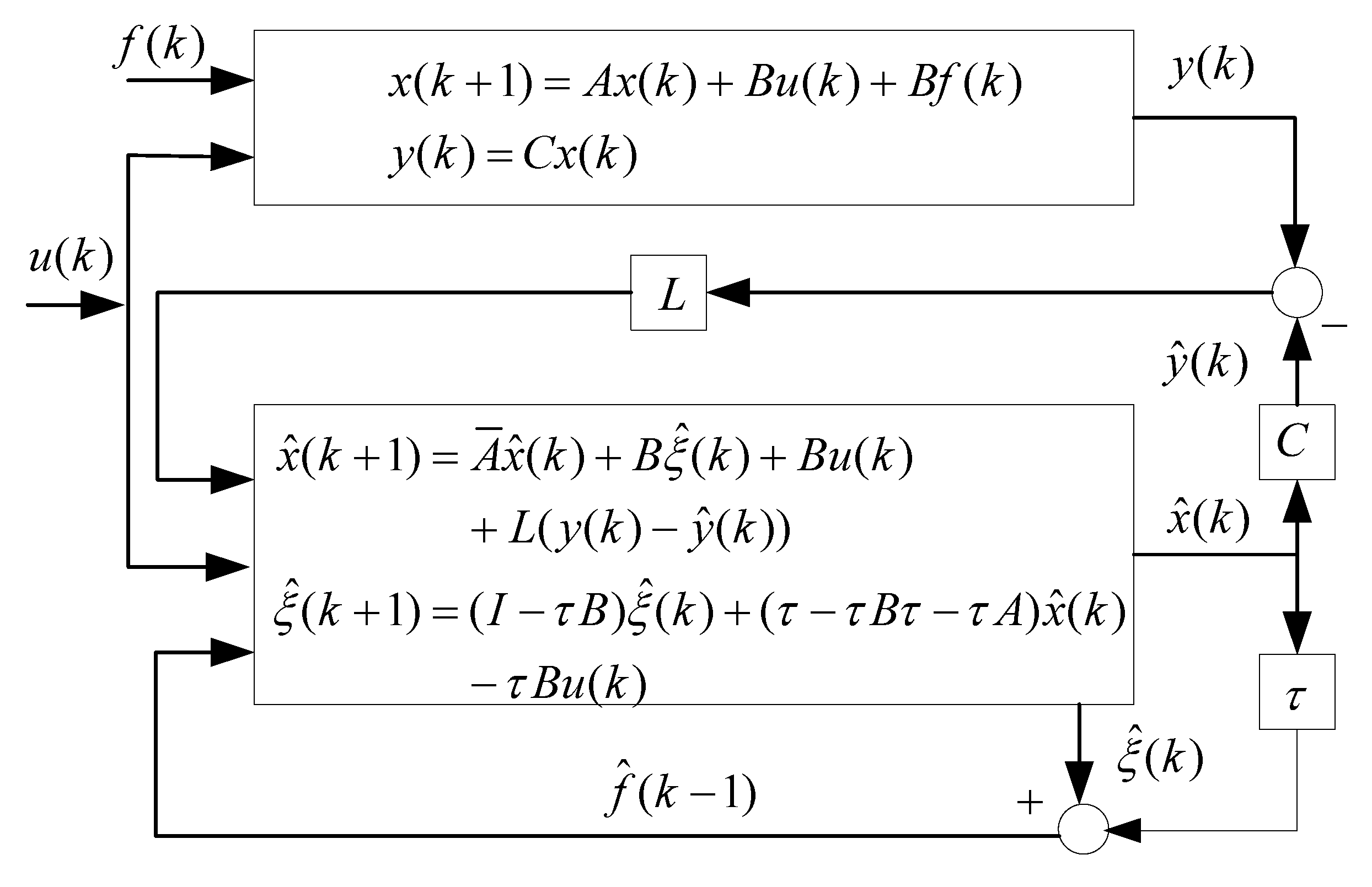
The fault-tolerant control structure based on an intermediate observer is shown in Figure 4.

Figure 4.
Fault-tolerant control based on intermediate observer.
The intermediate observer gain is a parameter that needs to be adjusted in the control algorithm. If the linear matrix inequality (LMI) has a solution, a larger can facilitate higher observer estimation accuracy. However, in this case, the control output may have overshot. A smaller will reduce the observer estimation accuracy of the system, but there will be no overshoot in the control system output. The stable convergence characteristic of fault-tolerant control algorithm can be proved by the following Theorem 1.
Theorem 1.
If there are scalars that satisfyand, and there are positive definite matrix, matrix, and scalarsatisfy
where,,,,, ,,,. Note that the positive definite matrixdoesn’t have to be determined in advance. The ‘lmivar’ function in the MATLAB software program can be used to calculate and solve the LMI problem for obtaining.
The state estimates of the global tracking error system (48) and (49) are uniformly bounded, which means thatandconverge toand, respectively.
Proof.
A Lyapunov function is taken as
where ; is a scalar.
The can be further obtained
According to Equations (54) and (55), it can be obtained
In order to simplify the calculation of and in the Equation (56). Based on the elimination lemma and Young’s inequality [23], the following relaxation inequality satisfies
where .
Defining , and combining the Equations (56)–(58), there are
According to Equations (52) and (59), it can be obtained
where , .
According to the equation (52), we have
Defining , which means that if then . We have
where is the largest eigenvalue of the matrix . The is the minimum eigenvalue of the matrix . Note that, implies and , and the above inequality can be satisfied by selecting the appropriate matrix and scalar . Compact set is defined as following
Define as the complement of compact set , we have
If , combining Equations (63) and (68), it can be obtained
According to Lyapunov theorem and Equation (64), and are uniformly bounded, and they converge to with an exponential rate greater than . In addition, the linear matrix (51), corresponding to , can be obtained by using Schur’s complement formula. The above is the proof process of the fault-tolerant control algorithm. □
5.2. Fault-Tolerant Model Predictive Control Based on Identification Model
The dead-zone block can weaken the excitation characteristics of input signals, which not only affects the estimation accuracy of model parameters, but also weakens the control effect of control input signals. The estimation effect of the intermediate observer will also be adversely affected. In order to solve this problem, according to the dead-zone model parameters, a dead-zone nonlinear compensator is introduced to compensate the dead-zone nonlinear block into a linear block through the origin. The transformed linear block and the dynamic linear block form the generalized linear system, and the MPC method will be used to design the controller. The model predictive control mainly includes prediction time domain and control time domain parameters [36]. The model predictive control formula with prediction time domain and control time domain can be expressed as
and
Using the matrix, it can be expressed as
The fault estimate can only be obtained at the moment. So, replace all with , and replace with .
In order to compensate the impact of the output noise on the system, the error is used as the compensation value. We have
The equation can also be expressed as
where , , ,
Define the following cost function
where is the weighted coefficient matrix of prediction error; is the weighted coefficient of control increment. A larger matrix value can make the control variable drive the state to the origin quickly, so as to reduce the control error. A larger value of allows the state to reach the origin at a slower speed by reducing the control amplitude.
The control increment sequence can be calculated by minimizing the cost function. Substitute Equation (74) into Equation (75), it can be obtained
where is the term unrelated to .
It can be transformed into a quadratic programming problem and expressed as
By optimizing the above problems, the optimal control rate can be obtained
By substituting the control rate into the control equation and solving it circularly, the MPC input can be obtained.
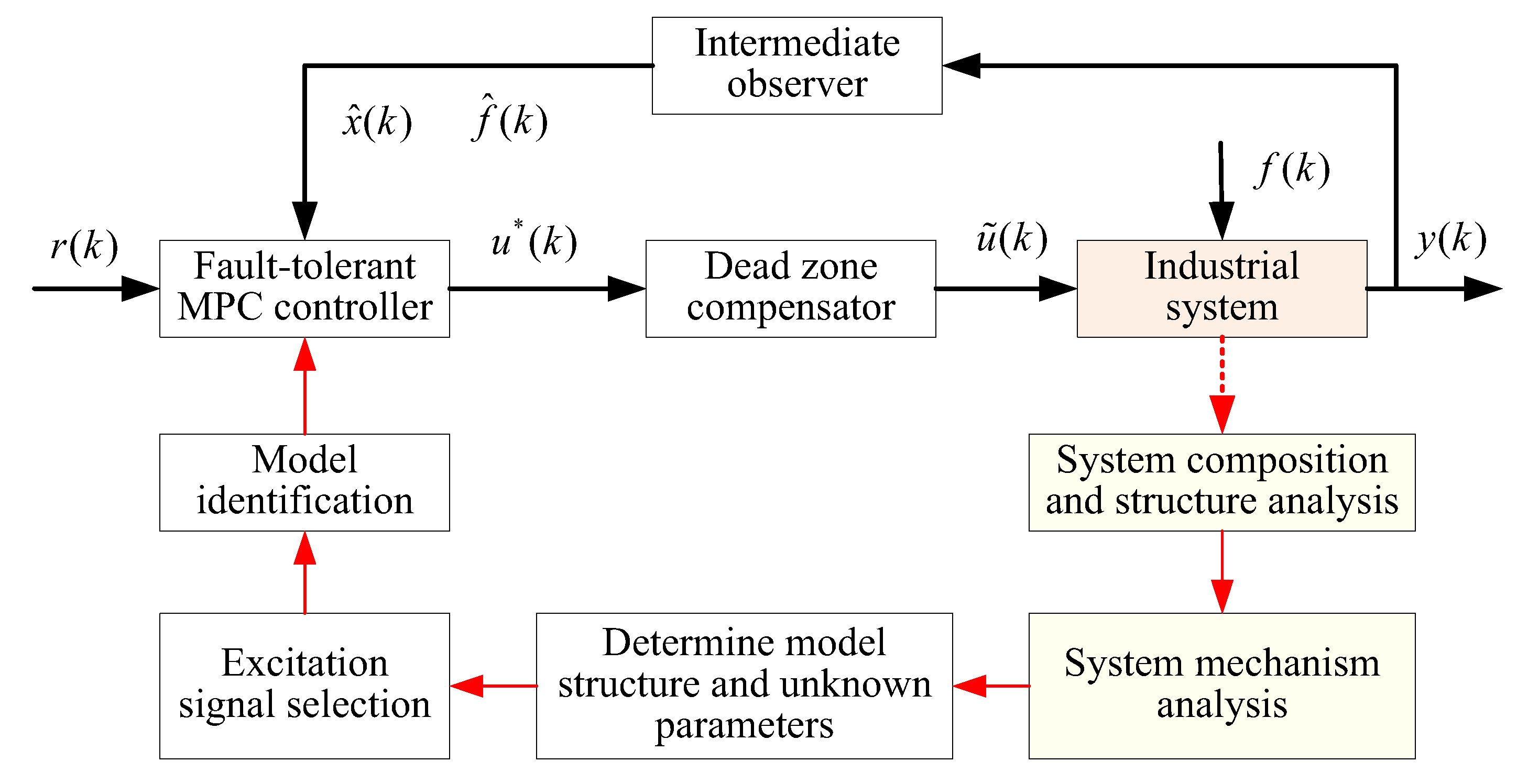
The schematic diagram of data-driven modelling and the fault-tolerant model predictive control strategy is shown in Figure 5. The proposed control scheme firstly obtains the estimated information of state and fault through the observer. Then, the controller is designed based on MPC technology. Therefore, the estimated information is obtained in advance of the control law. Observer and controller are not in a parallel relationship, but a progressive relationship. Only when the estimated information is convergent, the control law can guarantee the system convergence. Moreover, the computation time of the proposed control method is less than the sampling time of the system, which can ensure that the running time of the algorithm is less than the actuator frequency. Therefore, the controller can converge effectively and stably in practical system application.
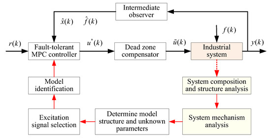
Figure 5.
Schematic diagram of data-driven modelling and fault-tolerant MPC strategy.
Note that the intermediate observer gain of the fault-tolerant control algorithm is a parameter that needs to be adjusted in the control algorithm. If is taken as a small parameter, the estimated performance will be reduced. If is taken as a large value, the estimation performance will be improved, but the overshoot will be increased. The prediction time domain and control time domain have different effects on the MPC algorithm. The prediction time domain is the prediction of the future time step, which represents the prediction degree of the controller for the future state. When the is taken as a large parameter value, the controller can predict the far future output information, but it will increase the prediction error and reduce the control accuracy. When the is taken as a small value, the control performance of changing signals will be reduced and the control will be unstable. An appropriate can enable the controller to modify the system input signal according to the current prediction error. The control time domain represents the number of control groups to be solved. The feedback correction controller applies only the first element of the control increment to the system. So, the numerical value of the has little influence on the control effect of the controller. In the proposed control algorithm, the prediction and control time domain parameters need to be manually adjusted according to the dynamic performance and identification model of the system.
6. Validation Examples
6.1. Numerical Example
Consider the following nonlinear system with dead-zone input nonlinearity
where the input signal is composed of several sinusoidal signals , which is used to persistently excite the system; is a white Gaussian noise with zero mean and variance , which causes signal-to-noise (SNR) = 14.3 dB and noise-to-signal (NSR) = 19.2%.
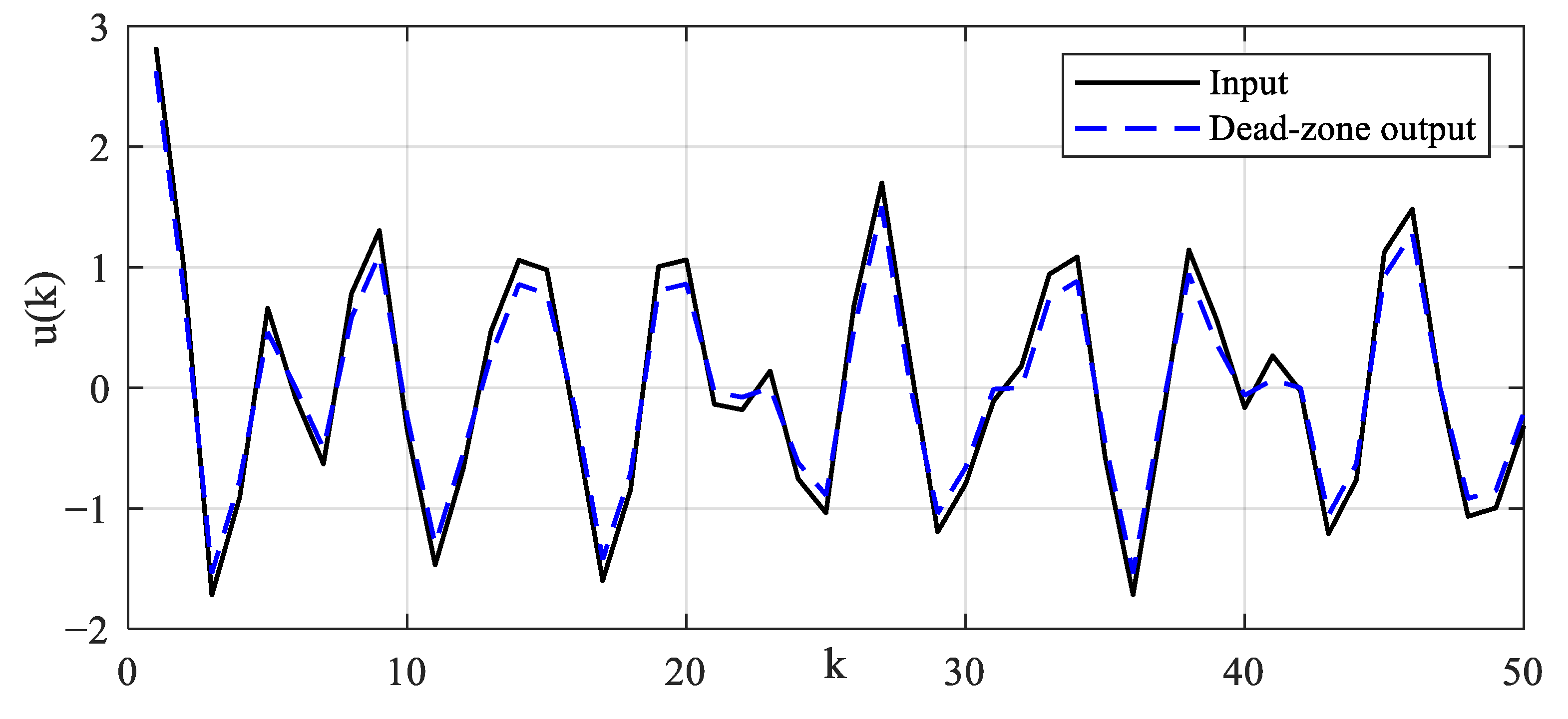
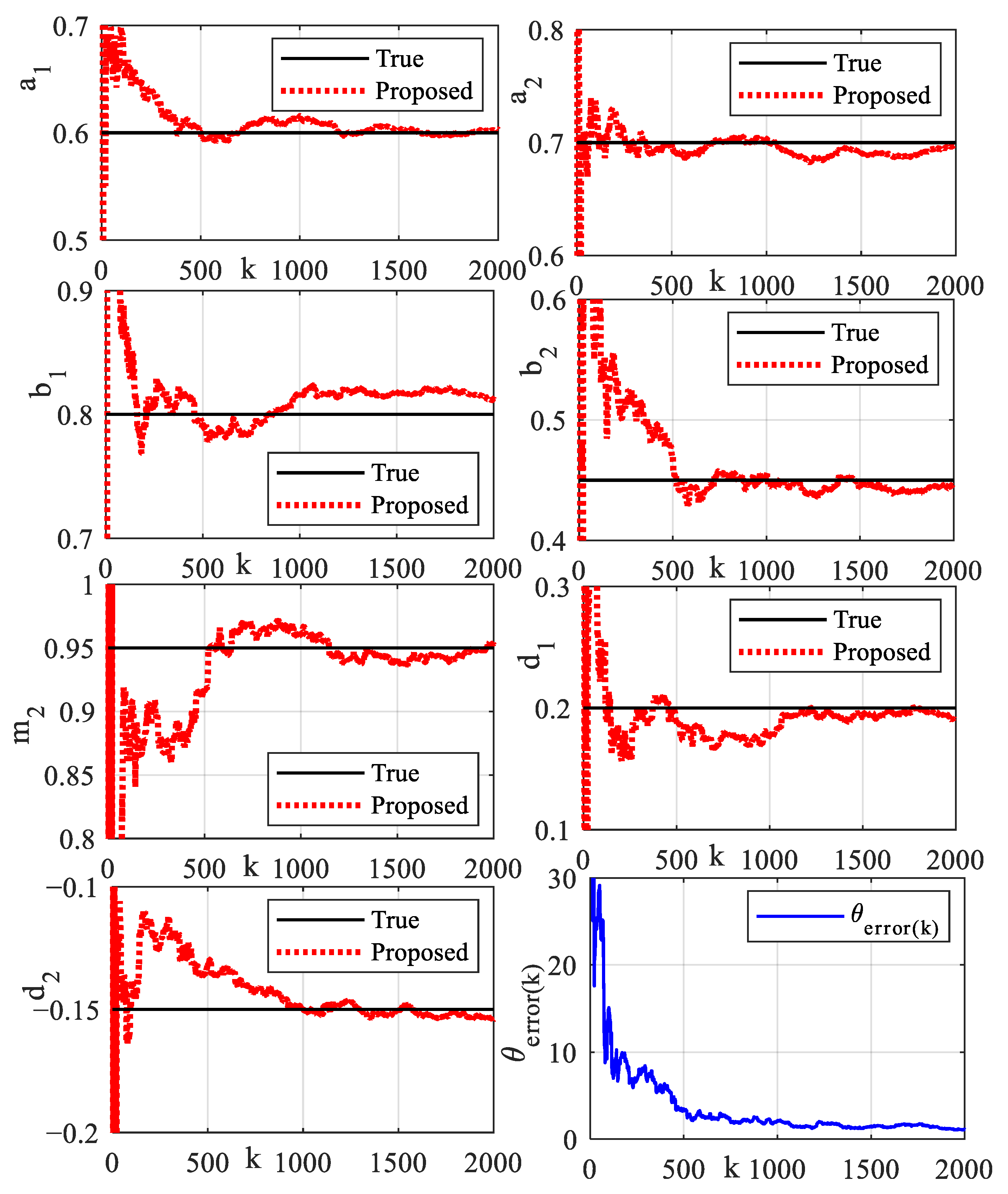
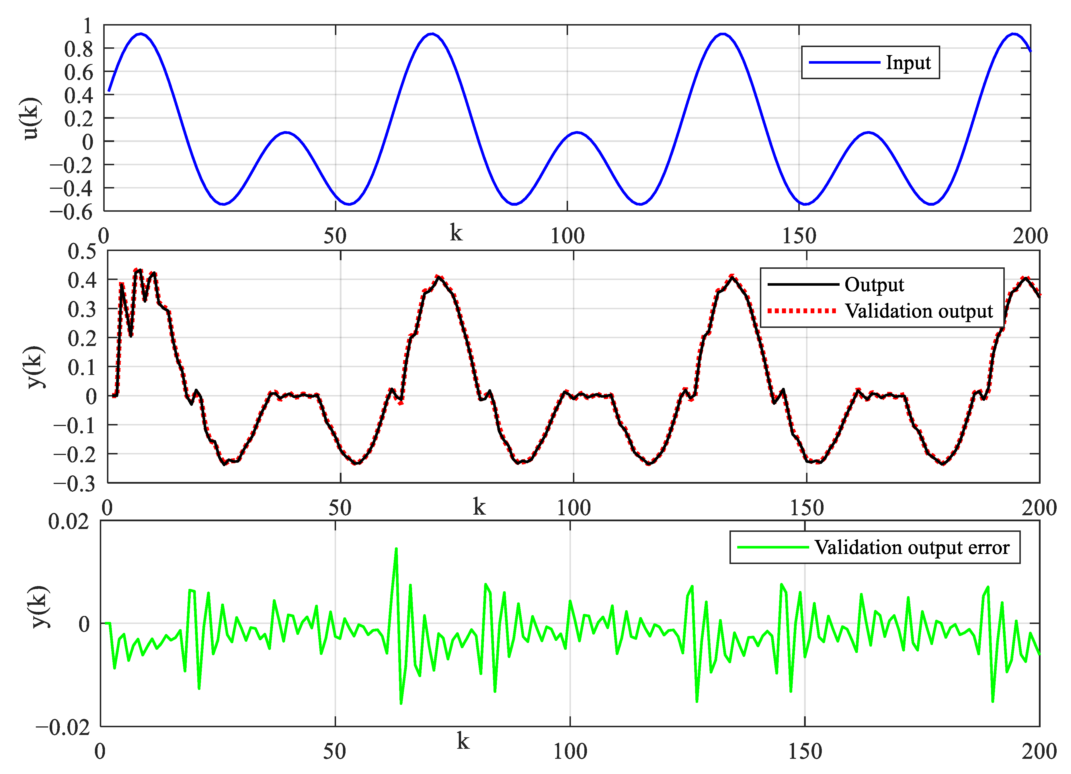
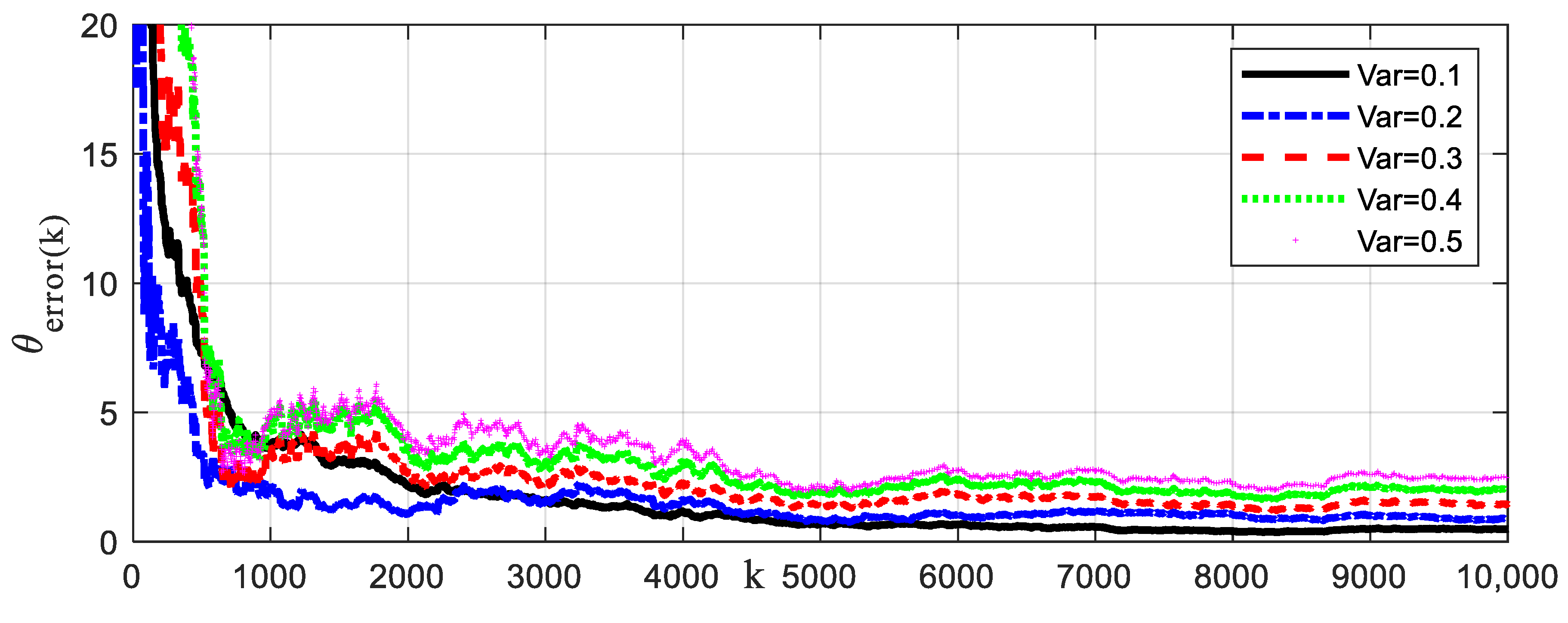
The system input signal and dead-zone output signal are illustrated, as shown in Figure 6. The sampling length of simulation data is specified as N = 2000. The parameter estimation error evaluation criterion is defined as . The estimation values of model parameters are shown in Table 2 and Table 3. The recursive parameter estimation results and estimation error are shown in Figure 7. The prediction output and error are shown in Figure 8. In order to cross-verify the performance of the model, the input signal is designed to excite the system. The input signal, validation output signal and output prediction error are shown in Figure 9. Output prediction error means and variances are shown in Table 4. To illustrate the robustness of the proposed algorithm, identification methods are tested under different noise levels. The sampling length of simulation data is specified as N = 10,000. The estimation results are shown in Figure 10. Parameter estimation error under different noise levels is shown in Table 5. The estimation results show that the identification model can describe the main dynamic characteristics of the system output, and the algorithm can converge stably. The established model can not only predict the output well, but also provide an accurate model reference for the system controller design and safe operation monitoring.
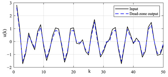
Figure 6.
Illustration diagrams of input and dead-zone output signal.

Table 2.
Parameter estimation results.

Table 3.
Parameter estimation results versus recursive step .
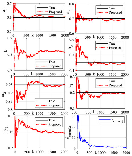
Figure 7.
Recursive parameter estimation and estimation error.
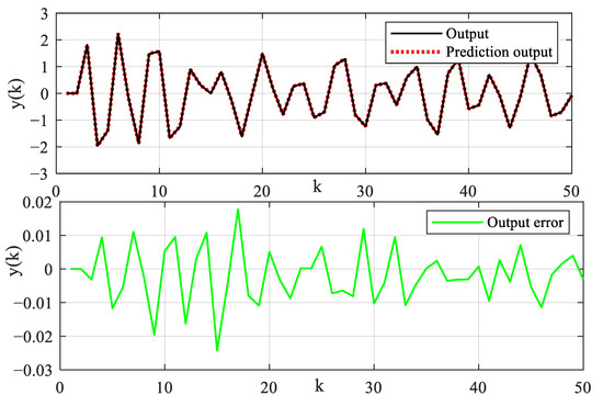
Figure 8.
Illustration diagrams of output and prediction error.

Figure 9.
Illustration diagrams of validation input and output error.

Table 4.
Output prediction error mean and variance.
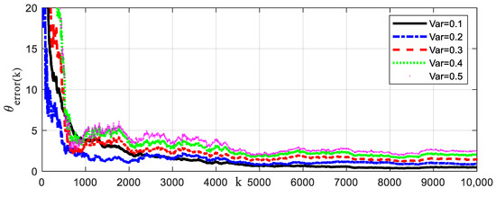
Figure 10.
Recursive curves of parameter estimation error under different noise levels.

Table 5.
Parameter estimation error under different noise levels (N = 10,000).
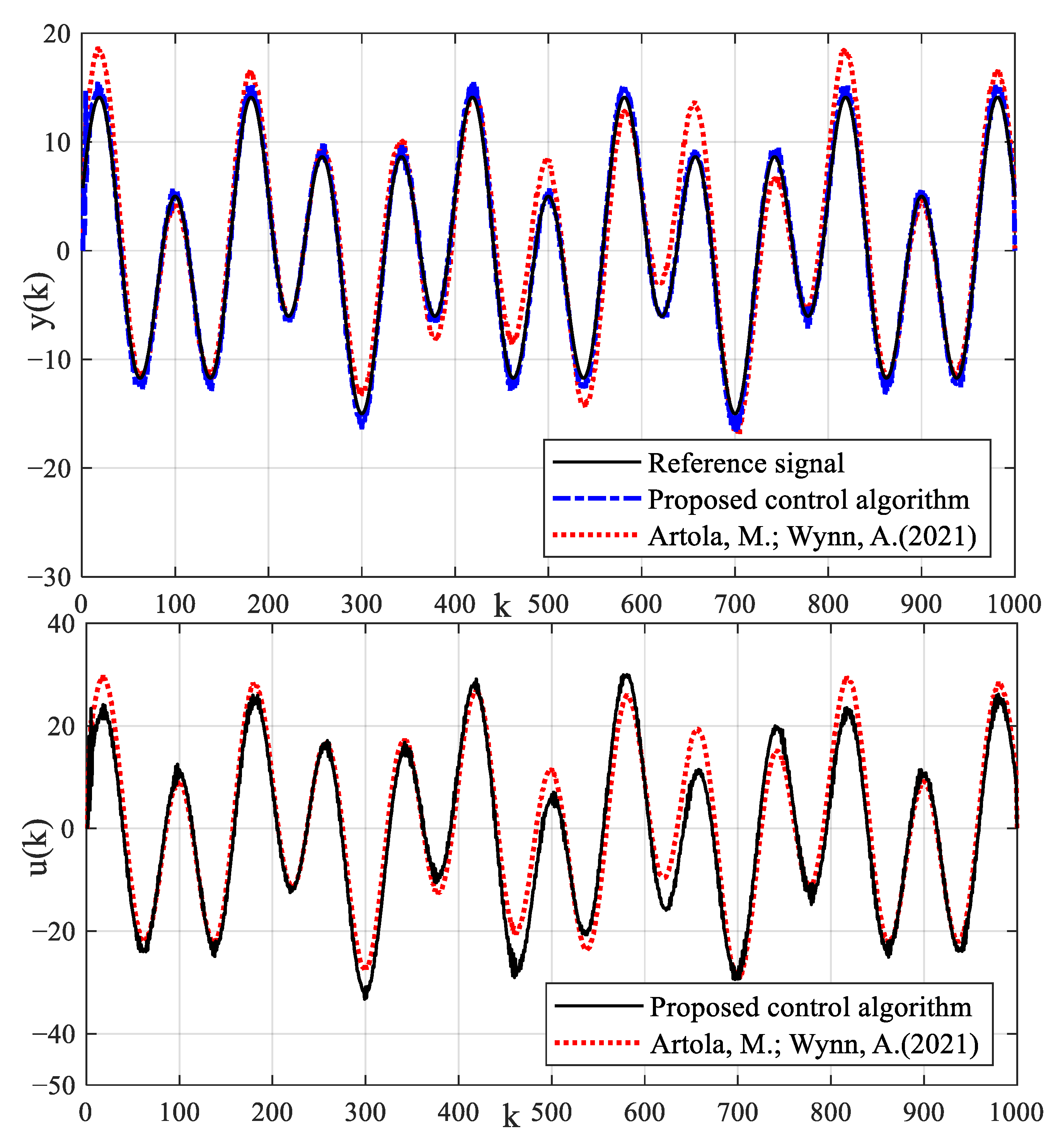
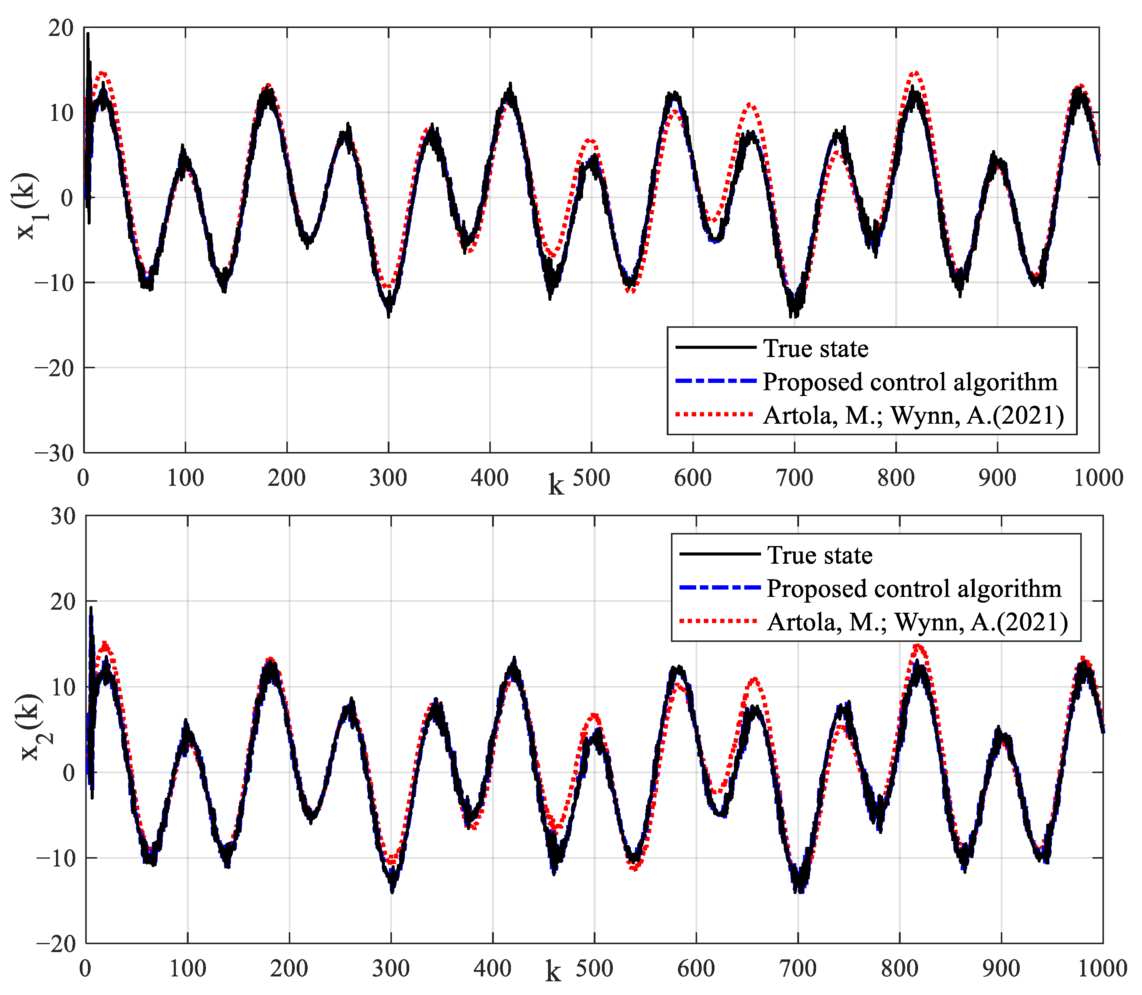
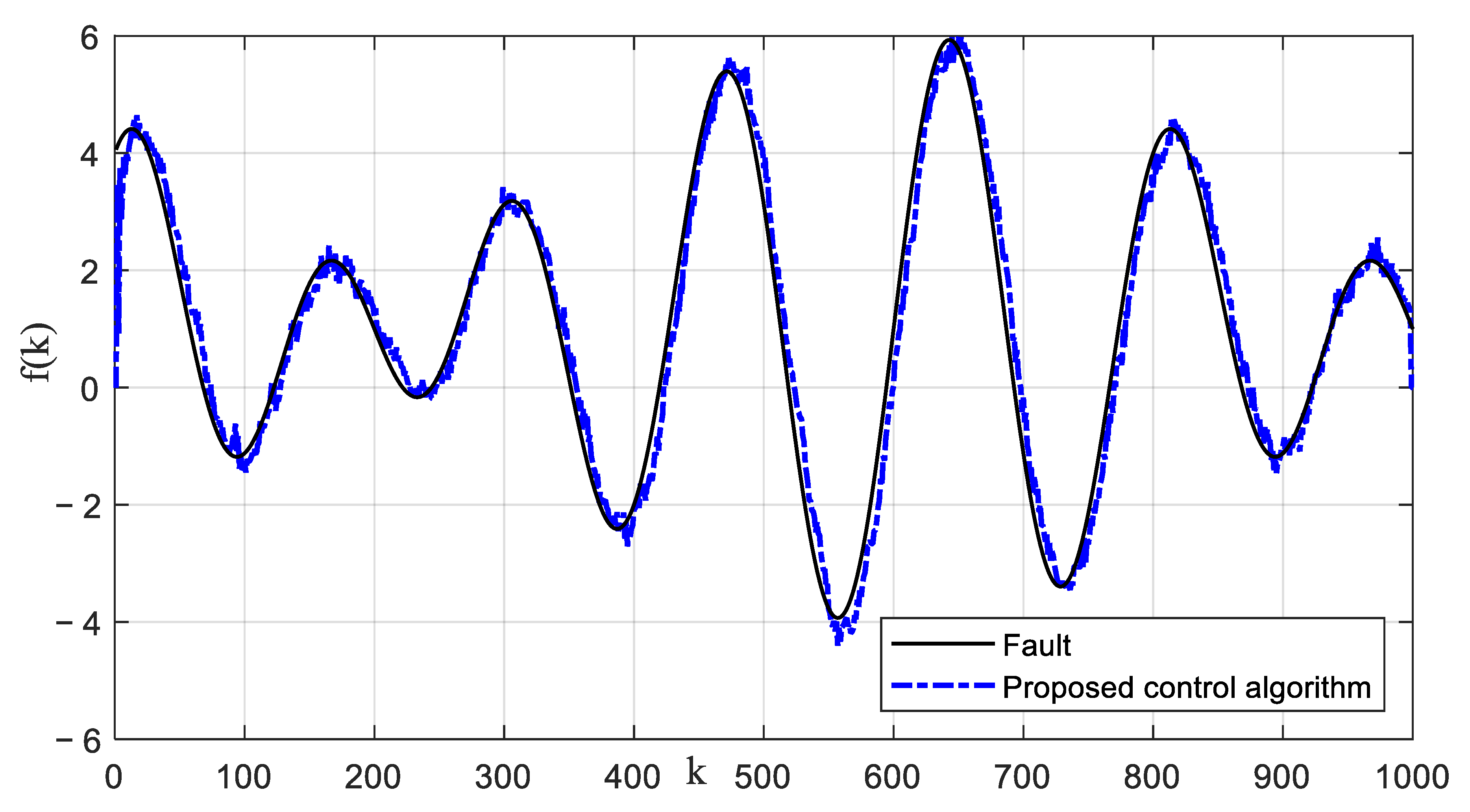
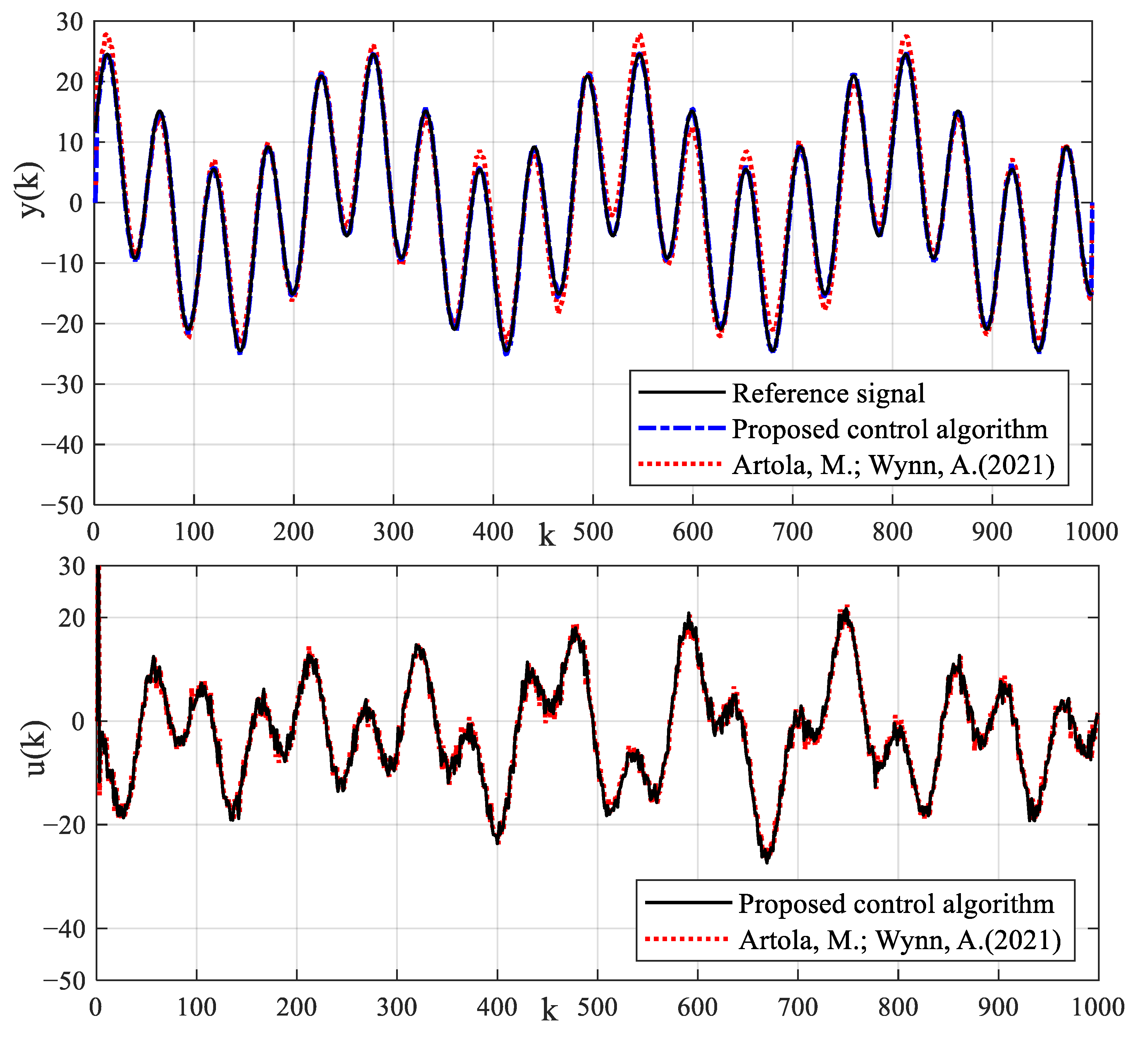
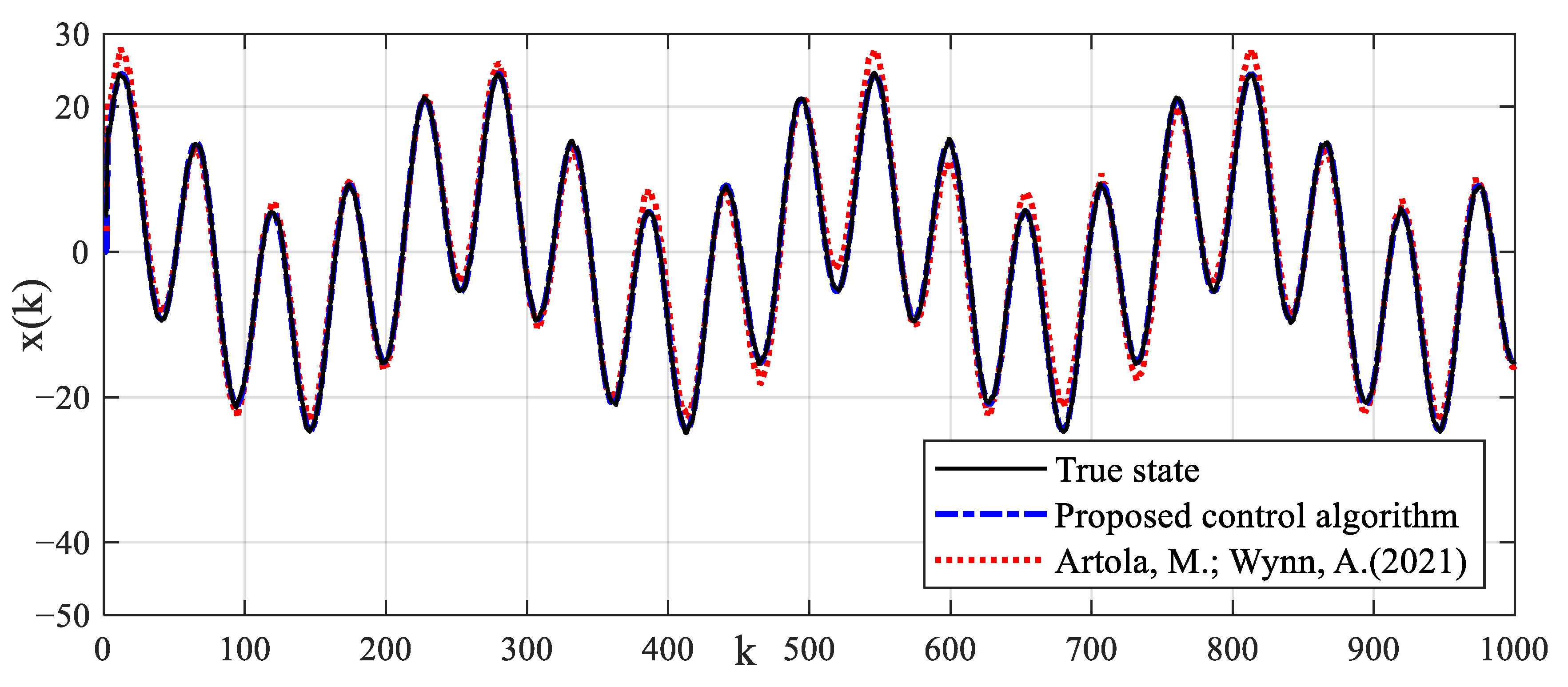
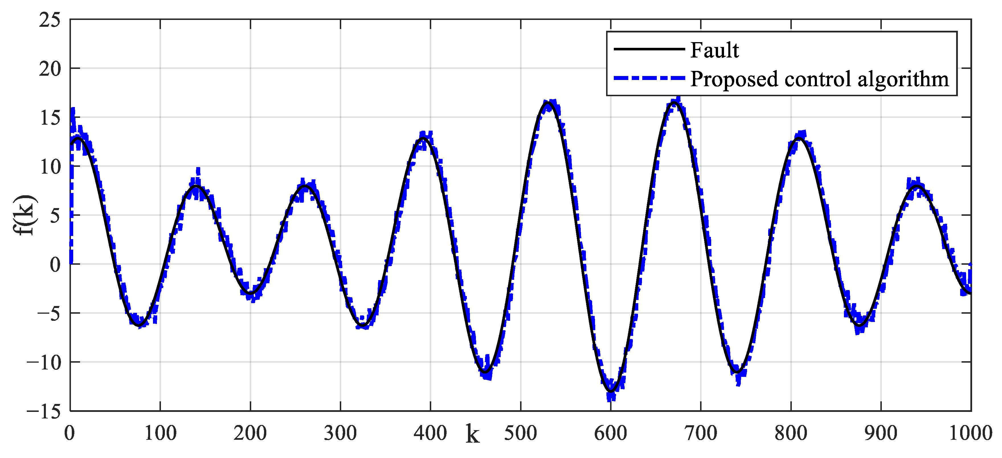
Based on the identification model, the robustness and theoretical significance of fault-tolerant model predictive control strategy will be verified. The system output control reference signal is taken as . The fault signal is taken as . The intermediate observer gain of the fault-tolerant control algorithm is taken as . In the model predictive control algorithm, the prediction time domain and control time domain are taken as and , respectively. The weighted coefficient matrix of the prediction error is taken as . The weighted coefficient of the control increment is taken as . The quadprog function of MATLAB is used to solve the cost function of MPC in Equation (75) to obtain the optimal control rate. In order to compare and verify the superiority of the control algorithm, the latest MPC algorithm proposed in Ref. [37] is also performed, which also has state feedback technology. The tracking control results and control input signals of different control algorithms for reference signals are shown in Figure 11. The tracking estimation results of status signals are shown in Figure 12. The tracking estimation result of fault signal is shown in Figure 13. It can be seen that the proposed control algorithm has better tracking control accuracy and stability.
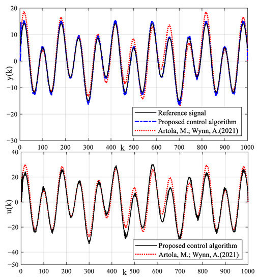
Figure 11.
Tracking control results of reference signal by using different control algorithms.
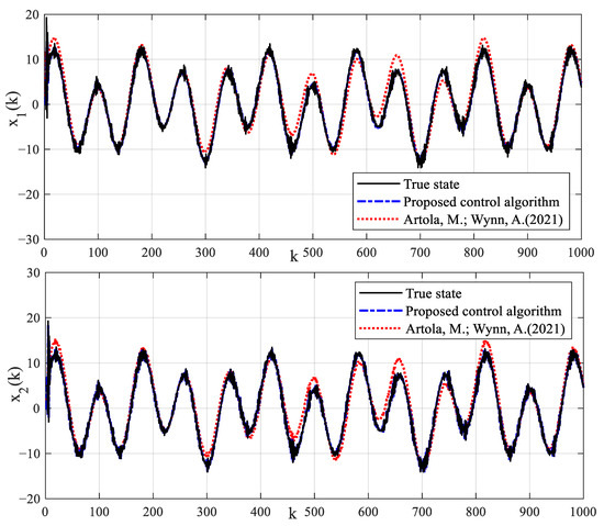
Figure 12.
Estimation results of state signal.
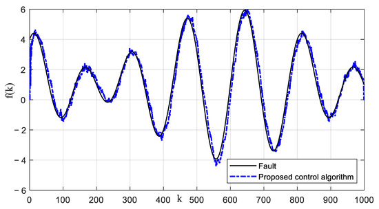
Figure 13.
Estimation result of fault signal.
Due to the existence of true model parameters in the numerical simulation example, the proposed identification algorithm can estimate parameters accurately. In addition, the proposed identification algorithm has strong robustness and good estimation accuracy for different noise levels. The estimated parameters of dead-zone can provide model basis for designing a dead-zone compensator. Although the control strategy in Ref. [37] is also a kind of model control strategy, it also compensates dead-zone parameters in simulation tests. Because there is no fault compensation, the control strategy in Ref. [37] cannot accurately track the reference signal and has a large control error in the dynamic control process with process fault. The state estimation results of the method in Ref. [37] have a large error. The control tracking error can cause production instability and product quality disqualification. The proposed control algorithm uses an intermediate observer to accurately estimate the fault signal. The fault-tolerant feedback control with fault estimation is used to compensate the fault signal. The compensation estimation strategy can improve the dynamic tracking performance of the proposed control algorithm. The precise control can not only improve product quality, but also ensure the safe and reliable operation of the production.
6.2. Experimental Test
The proposed modeling strategy is tested in the industrial actuator system of our laboratory. The system input is the target torque (unit: one rated torque in a thousand) stored in the register. In order to excite the system persistently, the composite input signal composed of sinusoidal signals of different frequencies and amplitudes is designed as
where ; ; .
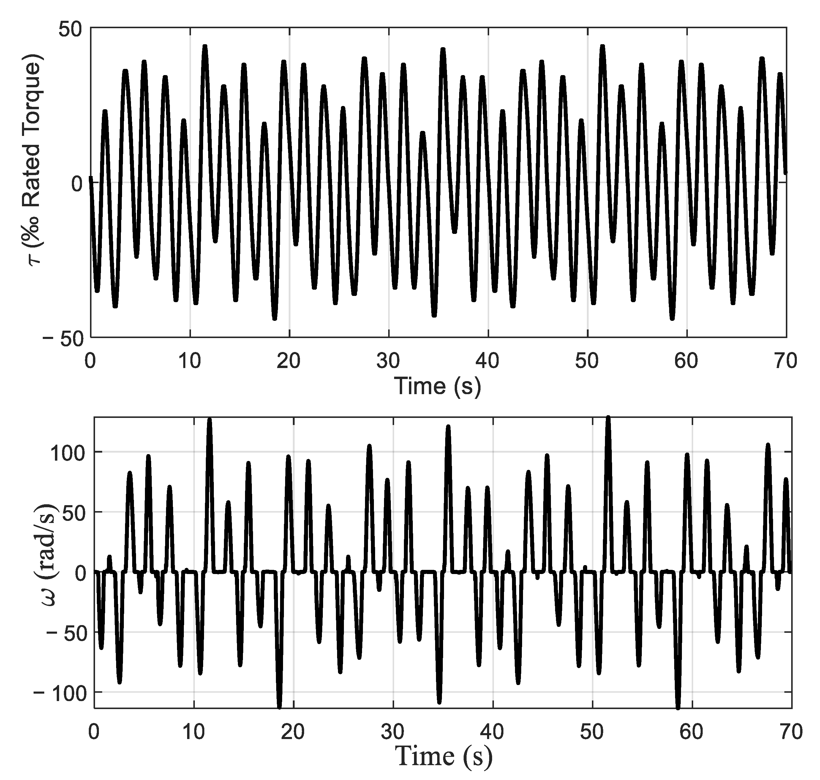
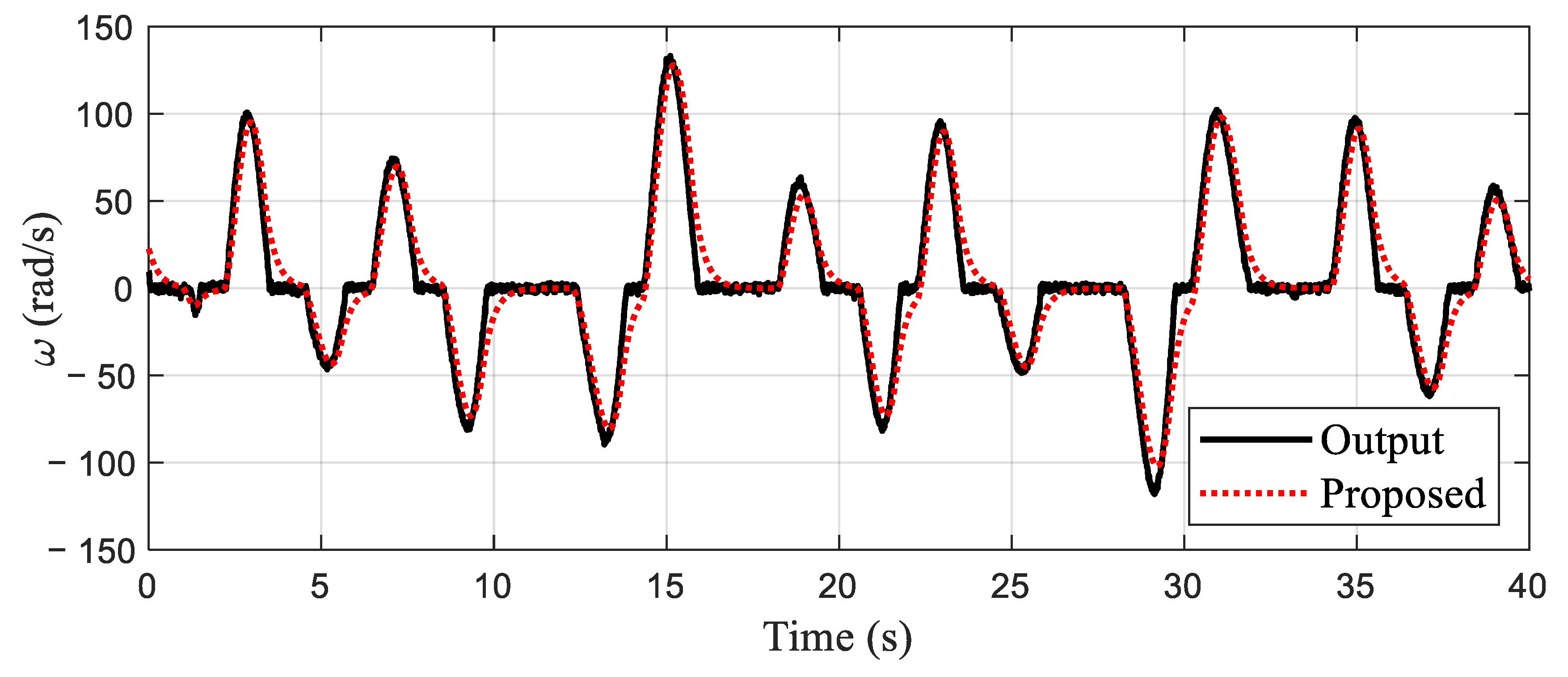
The system output is velocity (unit: radians per second, rad/s). The portion of input and output data at the sampling frequency of 100 Hz are shown in Figure 14. The identification algorithm is used to estimate the experimental system by using 5000 points of ample data. The parameter estimation results are shown in Table 6, and the estimation is . The model prediction output is shown in Figure 15. It can be seen that the identification model can reflect the dynamic characteristics of the system well. The identification model can be expressed as
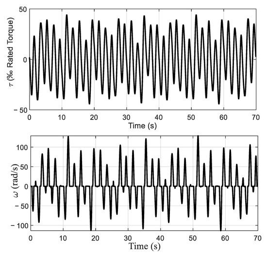
Figure 14.
Input and output experimental signal illustration diagram.

Table 6.
Estimation results of experimental system.
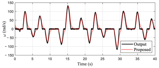
Figure 15.
Output prediction on experimental platform.
The system output control reference signal is taken as . The fault signal is taken as . The observer gain is taken as . The prediction time domain and control time domain are taken as and , respectively. The weighted coefficient matrix of the prediction error is taken as . The weighted coefficient of the control increment is taken as . The control algorithm in Ref. [37] is also performed. The tracking control results and control input signals of different control algorithms for reference signals are shown in Figure 16. The tracking estimation results of status signals are shown in Figure 17. The tracking estimation of the fault signal is shown in Figure 18. It can be seen that the proposed control algorithm has better tracking accuracy and stability. The control strategy in Ref. [37] cannot accurately track the reference signal. The state estimation results of the method in Ref. [37] have a large error.
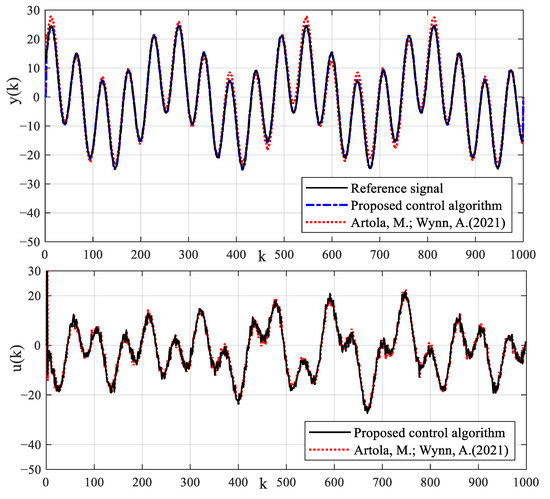
Figure 16.
Tracking control results of reference signal by using different control algorithms.
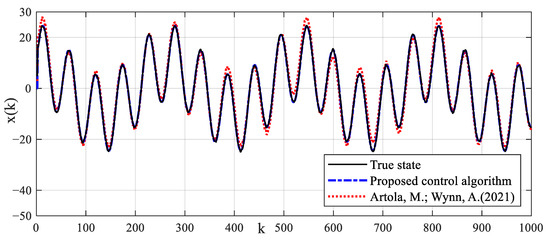
Figure 17.
Estimation results of state signal.
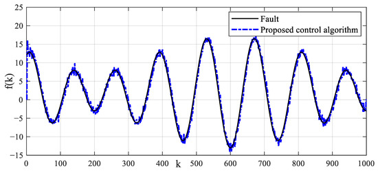
Figure 18.
Estimation result of fault signal.
In the actual experimental test, the true parameters of the model cannot be known, although the identification parameters converge stably. However, it is impossible to compare the estimation errors of parameters. The estimated identification model can well reflect the dynamic output performances of the system as shown in Figure 15, which satisfies the practical application criteria of the identification algorithm. Compared with the mechanism modeling method and the intelligent modeling method, the proposed identification modeling method is simple and easy to apply. The identified model provides a good model basis for the proposed model-based control strategy. It can be seen from the results of identification estimation that the dead-zone parameters of the test platform are large. Dead-zone parameters cannot be treated as time-delay parameters or input disturbances. The dead-zone may greatly reduce the excitation of small input control signals to the system. The dead-zone may also reduce the tracking control effect of the proposed control algorithm and control strategy in Ref. [37]. Based on the identification model, a dead-zone compensator is constructed, which transform the nonlinear system with dead-zone input into a generalized linear system. This strategy reduces the difficulty of process control. Process fault will reduce the estimation precision of intermediate state and the dynamic tracking accuracy of control algorithm. Due to the lack of fault estimation and compensation technology, it is difficult for the control strategy in Ref. [37] to accurately estimate the intermediate state and track the dynamic reference signal in the application of the process with faults as shown in Figure 16 and Figure 17. Imprecise control results will reduce the production accuracy of industrial actuator systems, resulting in difficult to produce qualified products, which may reduce the competitive advantage of enterprises. The proposed model-based control strategy utilizes the potential of the identification model and compensates process faults with an intermediate observer, which ensures precise dynamic tracking control. In the process control, the process fault is compensated dynamically and in a timely fashion, which guarantees production stability and product quality. In addition, the closed-loop control strategy based on MPC can also eliminate the influence of random measurement noise. These are the advantages and characteristics of the proposed identification modeling and fault-tolerant predictive control strategy. The superiority and applicability of the proposed modeling and control strategy are verified by the experimental test results.
7. Conclusions
The industrial actuator system has the nonlinear characteristics of dead-zone input, which may weaken the excitation characteristics of the input signal. The structure and order of the system model are determined by analyzing the mechanism relationship between input torque and output angular velocity. A Hammerstein nonlinear model with a dead-zone nonlinear block and a linear dynamic block in series has been used to fit the system output. Under the framework of least squares, an online parameterized estimation method is proposed, and the convergence of the algorithm is also analyzed. The identification model can describe the main dynamic characteristics of the system output. The cutoff effect of dead-zone input reduces the persistently exciting characteristics of the input signal and the information vector. The information vector contains unknown dead-zone parameters. An intermediate observer has been used to estimate the process faults signal. A fault-tolerant synchronous control feedback rate based on fault estimation has been designed to compensate faults. In order to eliminate the weakening effect of the dead-zone block on the control signal, a compensator has been introduced to transform the dead-zone function into a linear function passing through the origin of coordinates based on the dead-zone identification model. The model predictive control strategy has been designed for the generalized linear system to achieve precise control. By comparing with the existing methods, the effectiveness and superiority of the proposed modeling and fault-tolerant control algorithms are verified by using the experimental platform and numerical example.
Author Contributions
Conceptualization, S.D. and Y.Z.; methodology, S.D.; software, Y.Z.; validation, S.D.; formal analysis, Y.Z.; investigation, Y.Z.; resources, S.D.; data curation, S.D.; writing—original draft preparation, S.D; writing—review and editing, Y.Z.; visualization, Y.Z.; supervision, S.D.; project administration, Y.Z.; funding acquisition, S.D. All authors have read and agreed to the published version of the manuscript.
Funding
The research was funded by the Jiangsu Provincial Natural Science Foundation of China under Grant No. BK20210493 and the Key Laboratory of Intelligent Textile and Flexible Interconnection of Zhejiang Province under Grant No. ZD03.
Data Availability Statement
The data that support the findings of this study are available from the corresponding author, Shi-jian Dong (shijiandong@cumt.edu.cn), upon reasonable request.
Conflicts of Interest
The authors declare that the manuscript does not involve any ethical issues, and we do not have any conflicts of interest.
References
- Zou, X.; Wang, F.; Pan, J. 3-D online modeling and assessment of operating performance for nonstationary industrial processes with nonlinearity. J. Process Control 2021, 101, 1–10. [Google Scholar] [CrossRef]
- Costa, T.V.; Sencio, R.R.; Oliveira-Lopes, L.C.; Silva, F.V. Fault-tolerant control by means of moving horizon virtual actuators: Concepts and experimental investigation. Control Eng. Pract. 2021, 107, 104683. [Google Scholar] [CrossRef]
- Liu, Y.; Feng, X.; Li, P.; Li, Y.; Su, Z.; Liu, H.; Lu, Z.; Yao, M. Modeling, Identification, and Compensation Control of Friction for a Novel Dual-Drive Hydrostatic Lead Screw Micro-Feed System. Machines 2022, 10, 914. [Google Scholar] [CrossRef]
- Mi, W.; Zheng, W.X. Adaptive Rational Orthogonal Basis Functions for Identification of Continuous-Time Systems. IEEE Trans. Autom. Control 2020, 66, 1809–1816. [Google Scholar] [CrossRef]
- Zhang, Q.; Wang, H.; Liu, C. MILM hybrid identification method of fractional order neural-fuzzy Hammerstein model. Nonlinear Dyn. 2022, 108, 2337–2351. [Google Scholar] [CrossRef]
- Teng, A.; Wu, Q.; Yang, T.; Sun, L.; Sun, N. X-Shaped Structure-Based Modeling and Control for a Stable Platform with a Series Elastic Actuator. Machines 2022, 10, 430. [Google Scholar] [CrossRef]
- Abreu, P.E.; Tavares, L.A.; Teixeira, B.O.; Aguirre, L.A. Identification and nonlinearity compensation of hysteresis using NARX models. Nonlinear Dyn. 2020, 102, 285–301. [Google Scholar] [CrossRef]
- Dai, J.; Chen, N.; Yuan, X.; Gui, W.; Luo, L. Temperature prediction for roller kiln based on hybrid first-principle model and data-driven MW-DLWKPCR model. ISA Trans. 2020, 98, 403–417. [Google Scholar] [CrossRef]
- Pappalardo, C.M.; Guida, D. System identification algorithm for computing the modal parameters of linear mechanical systems. Machines 2018, 6, 12. [Google Scholar] [CrossRef]
- Yu, M.; Guo, G.; Liu, J.; Shang, L. Closed-loop time-varying continuous-time recursive subspace-based prediction via principle angles rotation. ISA Trans. 2022, 122, 135–145. [Google Scholar] [CrossRef]
- Mi, W.; Rao, H.; Qian, T.; Zhong, S. Identification of discrete Hammerstein systems by using adaptive finite rational orthogonal basis functions. Appl. Math. Comput. 2019, 361, 354–364. [Google Scholar] [CrossRef]
- Palkin, G.; Suvorov, I. Simulation Modeling of First Rise Section of Water Supply System with Installed Complex of Automatic Pump Performance Control. Machines 2021, 9, 63. [Google Scholar] [CrossRef]
- Dong, S.; Yu, L.; Zhang, W.A.; Chen, B. Robust extended recursive least squares identification algorithm for Hammerstein systems with dynamic disturbances. Digit. Signal Process. 2020, 101, 102716. [Google Scholar] [CrossRef]
- Chen, F.; Young, P.C. A simple robust method of fractional time-delay estimation for linear dynamic systems. Automatica 2022, 137, 110117. [Google Scholar] [CrossRef]
- Du, N.; Zhang, L.; Long, X.; Yang, X.; Yu, F. Recursive identification for choke finger system in wind tunnel. ISA Trans. 2020, 107, 173–180. [Google Scholar] [CrossRef] [PubMed]
- Giri, F.; Rochdi, Y.; Chaoui, F.Z. Hammerstein systems identification in presence of hard nonlinearities of preload and dead-zone type. IEEE Trans. Autom. Control 2009, 54, 2174–2178. [Google Scholar] [CrossRef]
- Hadid, B.; Duviella, E.; Lecoeuche, S. Data-driven modeling for river flood forecasting based on a piecewise linear ARX system identification. J. Process Control 2020, 86, 44–56. [Google Scholar] [CrossRef]
- Yu, F.; Mao, Z.; Jia, M. Recursive identification for Hammerstein–Wiener systems with dead-zone input nonlinearity. J. Process Control 2013, 23, 1108–1115. [Google Scholar] [CrossRef]
- Na, J.; He, H.; Huang, Y.; Dong, R. Adaptive estimation of asymmetric dead-zone parameters for sandwich systems. IEEE Trans. Control Syst. Technol. 2021, 30, 1336–1344. [Google Scholar] [CrossRef]
- Ding, S.X. Advanced Methods for Fault Diagnosis and Fault-Tolerant Control; Springer: Berlin/Heidelberg, Germany, 2021. [Google Scholar]
- Deng, C.; Yang, G.H. Distributed adaptive fault-tolerant control approach to cooperative output regulation for linear multi-agent systems. Automatica 2019, 103, 62–68. [Google Scholar] [CrossRef]
- Ning, X.; Zhang, Y.; Wang, Z.; Yu, D.; Guo, H.; Mei, H. BLS-based adaptive fault tolerant control for a class of space unmanned systems with time-varying state constraints and input nonlinearities. Eur. J. Control 2021, 61, 1–12. [Google Scholar] [CrossRef]
- Yang, X.; Gao, J.; Li, L.; Luo, H.; Ding, S.X.; Peng, K. Data-driven design of fault-tolerant control systems based on recursive stable image representation. Automatica 2020, 122, 109246. [Google Scholar] [CrossRef]
- Zhao, Z.; Liu, Z.; He, W.; Hong, K.S.; Li, H.X. Boundary adaptive fault-tolerant control for a flexible Timoshenko arm with backlash-like hysteresis. Automatica 2021, 130, 109690. [Google Scholar] [CrossRef]
- Li, Z.; Yang, G.H. Integrated design of event-triggered closed-loop subspace predictive control scheme. IEEE/ASME Trans. Mechatron. 2017, 23, 80–88. [Google Scholar] [CrossRef]
- Guo, G.; Wang, Y. An integrated MPC and deep reinforcement learning approach to trams-priority active signal control. Control Eng. Pract. 2021, 110, 104758. [Google Scholar] [CrossRef]
- Xie, S.; Xie, Y.; Gui, W.; Yang, C. Weighted-coupling CSTR modeling and model predictive control with parameter adaptive correction for the goethite process. J. Process Control 2018, 68, 254–267. [Google Scholar] [CrossRef]
- He, D.; Wang, L.; Sun, J. On stability of multiobjective NMPC with objective prioritization. Automatica 2015, 57, 189–198. [Google Scholar] [CrossRef]
- Galuppini, G.; Magni, L.; Raimondo, D.M. Model predictive control of systems with deadzone and saturation. Control Eng. Pract. 2018, 78, 56–64. [Google Scholar] [CrossRef]
- Zhang, B.; Mao, Z. Adaptive control of stochastic Hammerstein systems with dead-zone input non-linearity. Trans. Inst. Meas. Control 2015, 37, 746–759. [Google Scholar] [CrossRef]
- Bernardi, E.; Adam, E.J. Fault-tolerant predictive control based on linear parameter varying scheme for industrial processes. J. Taiwan Inst. Chem. Eng. 2021, 129, 1–14. [Google Scholar] [CrossRef]
- Ren, Y.; Zhu, P.; Zhao, Z.; Yang, J.; Zou, T. Adaptive fault-tolerant boundary control for a flexible string with unknown dead zone and actuator fault. IEEE Trans. Cybern. 2021, 52, 7084–7093. [Google Scholar] [CrossRef]
- Keller, R.; Ding, S.X.; Müller, M.; Stolten, D. Fault-tolerant model predictive control of a direct methanol-fuel cell system with actuator faults. Control Eng. Pract. 2017, 66, 99–115. [Google Scholar] [CrossRef]
- Qu, S.; He, T.; Zhu, G.G. Engine EGR valve modeling and switched LPV control considering nonlinear dry friction. IEEE/ASME Trans. Mechatron. 2020, 25, 1668–1678. [Google Scholar] [CrossRef]
- Pang, Z.H.; Xia, C.G.; Zhai, W.F.; Liu, G.P.; Han, Q. Networked active fault-tolerant predictive control for systems with random communication constraints and actuator/sensor faults. IEEE Trans. Circuits Syst. II Express Briefs 2021, 69, 2166–2170. [Google Scholar] [CrossRef]
- Heshmati-alamdari, S.; Eqtami, A.; Karras, G.C.; Dimarogonas, D.V.; Kyriakopoulos, K.J. A self-triggered position based visual servoing model predictive control scheme for underwater robotic vehicles. Machines 2020, 8, 33. [Google Scholar] [CrossRef]
- Artola, M.; Wynn, A.; Palacios, R. Modal-Based Nonlinear Model Predictive Control for 3-D Very Flexible Structures. IEEE Trans. Autom. Control 2021, 67, 2145–2160. [Google Scholar] [CrossRef]
Disclaimer/Publisher’s Note: The statements, opinions and data contained in all publications are solely those of the individual author(s) and contributor(s) and not of MDPI and/or the editor(s). MDPI and/or the editor(s) disclaim responsibility for any injury to people or property resulting from any ideas, methods, instructions or products referred to in the content. |
© 2023 by the authors. Licensee MDPI, Basel, Switzerland. This article is an open access article distributed under the terms and conditions of the Creative Commons Attribution (CC BY) license (https://creativecommons.org/licenses/by/4.0/).

