ML-Enabled Piezoelectric-Driven Internal Defect Assessment in Metal Structures

Abstract

With the growth of 3D printing in the production space, it is inevitable that quality assurance will be needed to keep final products within the constraints of requirements. Also, the variety of materials that can be used with 3D printing has increased over the years. Testing also must consider the process of manufacturing. This paper focuses its efforts on the finished product and not the process of manufacturing. Ultrasonic testing is a type of nondestructive testing. The experiments performed in this study aim to explore the usefulness of ultrasonic testing in materials that are 3D printed. The two materials used in this study are steel alloy metals and aluminum blocks of the same dimensions—120 mm × 40 mm × 15 mm. These materials represent common choices in additive manufacturing processes. The chosen alloys, such as Aluminum (6063T6) and grade-304 stainless steel, possess distinct properties crucial for validating the proposed testing method. Metal 3D-printed materials play a pivotal role in diverse industries, since ensuring their structural integrity is imperative for reliability and safety. Testing is crucial to identify and mitigate defects that could compromise the functionality and longevity of the final products, especially in applications with demanding performance requirements. An ultrasonic transducer is used to scan for subsurface defects within the samples and an oscilloscope is used to analyze the signals. Furthermore, several Machine Learning (ML) techniques are used to estimate the severity of the defects. The application of Machine Learning methods in the manufacturing industry has proven advantageous in terms of detecting defects due to its practicality and wide application. Due to their distinct benefits in processing image information, convolutional neural networks (CNNs) are the preferred method when working with picture data. In order to perform binary and multi-class classification, support vector machines that employ the alternative kernel function are a viable option for processing sensor signals and picture data. The study reveals that ultrasonic tests are viable for metallic materials. The primary objective of this work is to evaluate and validate the application of ultrasonic testing for the inspection of 3D-printed steel alloy metals and aluminum blocks. The novelty lies in the integration of Machine Learning techniques to estimate defect severity, offering a comprehensive and non-invasive approach to quality assessment in 3D-printed materials. The proposed method can successfully detect the presence of internal defects in objects, as well as estimate the location and severity of the defects.

1. Introduction

Additive Manufacturing (AM), commonly known as 3D printing, has undergone a remarkable evolution since its inception in the 1980s [1]. Initially conceived as a prototyping tool, in the form of Material Extrusion (MEX) [2,3,4], it has rapidly transitioned into a viable method for production. This transformation has underscored the critical need to ensure the quality of AM-produced materials, particularly with regard to the detection of defects like holes and voids. Despite numerous quality assessment methods available, Non-Destructive Testing (NDT) techniques have remained under-explored [5]. NDT, as a non-invasive testing approach, offers great potential for assessing the structural integrity of AM components without causing any damage [6].

Additive manufacturing has a lot of potential when compared to other manufacturing methods. This is partly due to the fast development of printer technologies and printable materials. The turnaround time for objects manufactured this way is faster. The feasibility of producing complex shapes is also much better than with other manufacturing methods.

In analyzing internal defects within a printed structure, several factors are considered, such as the type of material used, the force acting on the structure (stress), and the strain (displacement) caused by the applied force. Metals are common materials used and will be of importance in validating the proposed method. More importantly, each metallic material used for 3D printing processes has its own elastic and thermal properties, as well as its respective sound velocity, as seen in

Table 1. Comparison of the physical properties of Aluminum, Brass, Titanium, and Stainless-Steel metals.

Properties	Metals
	Aluminum (6063T6) [7]	Brass [8]	Titanium (Ti64) [9,10]	Stainless Steel (Grade-304) [11]
Density (g/${\mathrm{cm}}^3$)	2.7	8.75	4.5	8
Melting Point (°C)	655	990	1670	1450
Elastic Modulus (GPa)	69.5	115	113.8	193
Elongation (%)	5	60	54	40
Tensile strength (MPa)	220	270	950	515
Yield strength (MPa)	190	69	880	205
Thermal conductivity (W/mK)	201	159	6.6	16.2
Sound Velocity (m/s)	6320	4430	6100	5800

.

1.1. Metallic Materials for 3D Printing

Metals are the main materials of interest for this study, as additive manufacturing has improved, and it is becoming more common to use this technique for complex metallic manufacturing. The common ways of manufacturing metallic parts using AM are Powder Bed Fusion (PBF) and Directed Energy Deposition (DED) [12].

The present research addresses a pressing concern within this context by investigating the effectiveness of ultrasonic piezoelectric transducers in detecting internal defects, specifically holes and voids, in 3D-printed metal structures. It recognizes the shortcomings of existing methods and the urgency of advancing defect detection in AM. As AM gains prominence as a manufacturing method, a critical knowledge gap has emerged, hindering the production of high-quality, defect-free components. This research bridges this gap by shedding light on the intricate interplay of materials, forces, and strains within AM structures and its impact on defect detection. Furthermore, it provides an in-depth analysis of various metallic materials commonly used in AM, underscoring their unique properties and applications. Among these materials, aluminum, titanium, and stainless steel emerge as favored choices [13].

Table 1 highlights up to eight major properties of interest when considering metals for 3D printing. Aluminum, titanium, and stainless steel are popular options for the additive manufacturing of metals [13]. To use these metals in 3D printing, Selective Laser Sintering (SLS) or Direct Metal Laser Sintering (DMLS) are methods employed in the industry.

Aluminum, for instance, stands out as an attractive option due to its abundance, versatility, and corrosion resistance [14,15]. Similarly, stainless steel, characterized by its exceptional strength, high ductility, and corrosion resistance, holds promise, particularly the Direct Metal Laser Sintering (DMLS) method [16]. However, effectively employing these materials in AM necessitates reliable defect detection techniques.

1.2. Non-Destructive Testing Methods for Defect Detection in Additive Manufacturing

There are several testing methods for additive manufacturing. Some of these are destructive and others are non-destructive [17]. Quality control in AM produces some unique challenges. These challenges arise from the uniqueness of how parts are produced in AM. The material is formed under conditions that vary spatially and temporarily across the entire structure [18].

Critically, this research identifies and addresses the shortcomings of existing defect detection methods. While Scanning Electron Microscopy (SEM) and visual inspection excel in identifying surface defects, techniques such as pulsed thermography and microwave imaging offer limited insights into internal defects [18,19]. The proposed method, utilizing ultrasonic transducers and pulse-echo technology, aims to rectify these limitations by providing a cost-effective and accurate solution. It not only detects defects but also classifies their size and position within the structure (

Table 2. A comparison of different NDT methods [17,18,19,20].

Techniques	Properties
	Application	Ease of Use	Cost	Surface Defects	Subsurface Defects
Microscopy	Non-Contact	Complex	High	✓	✗
Visual Inspection	Non-Contact	Complex	Moderate	✓	✗
Pulsed Thermography	Non-Contact	Simple	Moderate	✗	✓
Microwave Imaging	Non-Contact	Complex	High	✓	✓
Ultrasonic Test	Contact	Simple	Low	✓	✓

).

1.3. The Integration of Machine Learning in Defect Classification

A notable trend in recent years is the integration of ML methods into NDT practices for defect classification and characterization. ML techniques have shown exceptional promise in handling large datasets and extracting valuable insights from sensor data [21]. Within the AM context, ML has been applied to estimate defect size, classify defects, and even predict component failure [22].

However, despite the increasing use of ML in AM quality control, there is a distinct lack of comprehensive comparisons between ML methods and traditional NDT techniques [23]. Such comparisons are crucial for identifying the most suitable ML algorithms for specific AM applications and defect types. Furthermore, understanding the limitations and advantages of ML in this context is essential for effective implementation.

Moreover, this research expands beyond defect detection to explore the role of Machine Learning (ML) methods in analyzing sensor data. With the growing importance of ML techniques in conjunction with NDT approaches for estimating defect size and dimensions [21,22], there arises a crucial need to compare their performance against traditional NDT techniques [23]. This paper takes up this challenge and conducts a comprehensive comparative analysis of five prominent supervised ML methods—Decision Trees (DT), Random Forests (RF), Logistic Regressions (LR), K-Nearest Neighbors (KNN), and Support Vector Machines (SVM). These methods are assessed not only for their proficiency in defect classification but also for their ability to classify defects into four categories: small, medium, large, and non-defect.

In essence, this research serves as a beacon in the AM landscape, addressing the drawbacks of previous methods and spearheading innovation in both NDT for AM quality control and the integration of ML for defect classification, particularly within the context of 3D-printed metal structures.

2. Materials and Methods

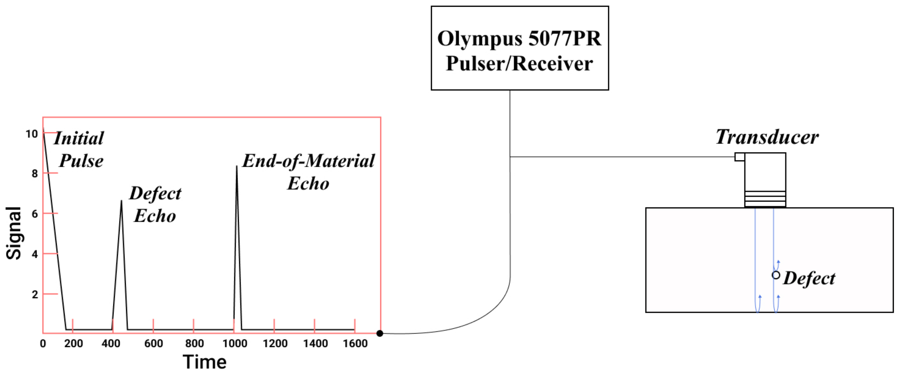
In ultrasonic testing, high-frequency sound energy is used for measuring and examining materials. Typically, an ultrasonic testing setup comprises a transmitter/receiver, a transducer, and a display unit to view the results [24]. The proposed method utilizes a pulser–receiver as the transmitter/receiver, and a delayed contact ultrasonic transducer is used to scan the objects under testing.

The pulser–receiver triggers the transducer, which is placed on the surface of the object, and high-frequency waves are sent through the material (pulse). When the waves encounter a change in the medium, such as a crack or a hole, a portion of the pulse is reflected back to the transducer (echo), while the rest continues traveling through the material, as shown in Figure 1.

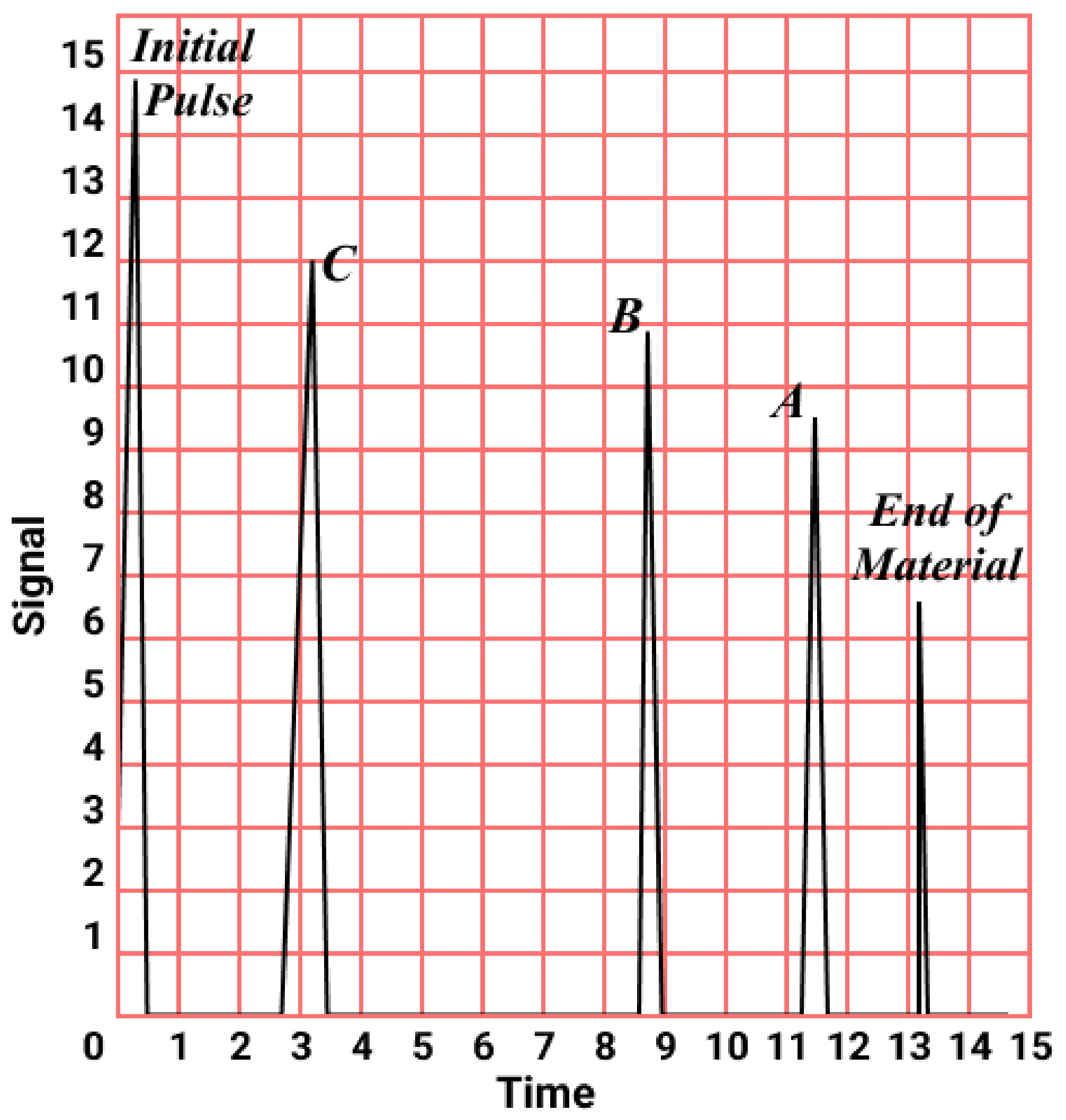
The echoes received by the transducer are sent via the pulser–receiver to the oscilloscope where the waveform can be observed. The visualization technique employed is the A-scan method [25], which represents the magnitude of echoes against time on a graph, as seen in Figure 2. The echoes are displayed in the order they are received by the transducer. In Figure 2, the first echo, C, is from the first defect encountered by the traveling wave, which is the largest of the three defects, and the third echo, A, is the last echo before the end of the material, representing the smallest of the three defects within the path of the traveling waves. The presence, size, and location of the defects can be analyzed based on the characteristics of the echoes. For instance, the decrease in signal strength is due to the size of the defect encountered by the waves. Echoes of higher amplitude signifies a larger defect as a large portion of the incident wave is reflected back to the transducer while the rest continue to travel through the material until another defect or end of material is encountered, as seen in Figure 2.

2.1. Test Bench Setup

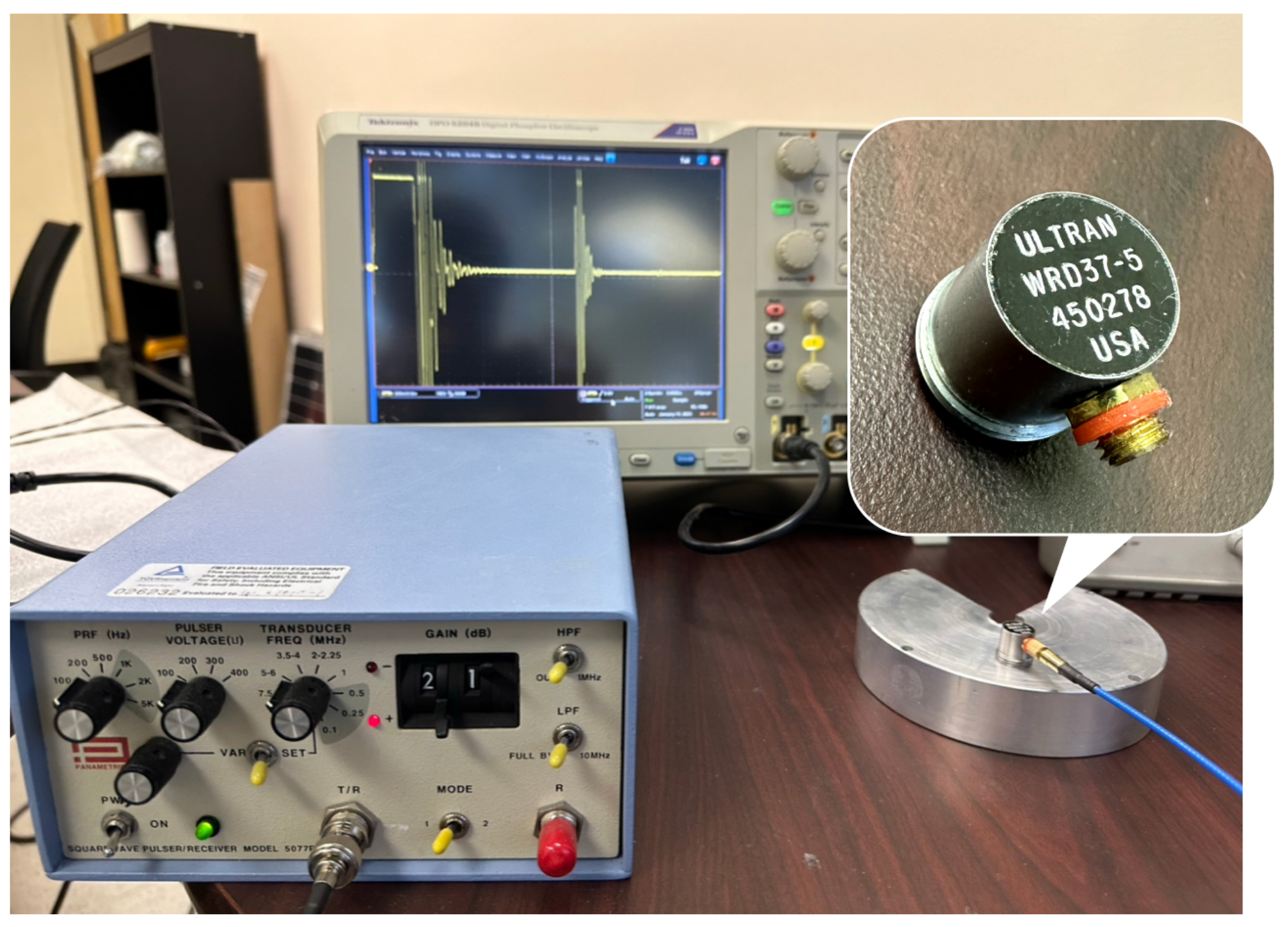
For the specific results presented in this paper, a 5 MHz transducer was used along with an Olympus pulser–receiver (Olympus, Waltham, MA, USA).The WRD37-5 (5 MHz) (Ultran, State College, PA, USA) transducer was manufactured by the ultran group, USA; the pulser–receiver is an Olympus squarewave pulser–receiver model 5077PR; and the oscilloscope is a Tektronix DPO 5204B Digital Phosphor Oscilloscope (Beaverton, OR, USA). On the pulser–receiver, the pulse-echo mode was selected and the pulse voltage was set to 100 V, as seen in the setup in Figure 3.

The corresponding transducer frequency was set on the pulser–receiver, along with a suitable gain value for a visible reading of the waveform. The selected transducer is usually determined by the nature and size of the defect. Firstly, the diameter of the transducer has to be significantly larger than the size of the defect. Secondly, the corresponding wavelength of the wave’s frequency in the material under test has to be smaller than the size of the defect to be detected. The wavelength can be computed using the following formula:

$$\lambda =\frac{v}{f}$$

(1)

where $\lambda$ is the wavelength, v is the sound velocity in that material (refer to Table 1 for values), and f is the transducer frequency. Repeating this computation for different transducer frequency values will provide enough information to select the appropriate transducer frequency for the test. For the purpose of this paper, sample A is made of stainless steel and sample B is made of aluminum. Referring to Table 1 in the previous section, $v_A$ is 5800 m/s and $v_B$ is 6320 m/s. Also, noting that the size of the smallest defect in this study is about 3 mm, the different transducer frequency values are listed in

Table 3. The calculated wavelengths for samples A and B for the respective frequency values.

F (MHz)	A (mm)	Verdict	B (mm)	Verdict
0.5	11.6	No	12.64	No
1	5.8	No	6.32	No
2	2.9	Yes	3.16	No
5	1.16	Yes	1.264	Yes
10	0.58	Yes	0.632	Yes

, which justifies the selection of the 5 MHz transducer. When dealing with known smaller defect sizes, transducers of higher frequency values should be employed for detection. In cases where the defect sizes are unknown, there will be a need to utilize multiple transducers of different frequency values until the defect is detected and readable on the oscilloscope.

The computed results indicated that only the 5 MHz and 10 MHz transducers were suitable for all the samples in this study based on the principle that the wavelength should be smaller than the defect size. Specifically, the wavelength values for both the 5 MHz and 10 MHz transducers were below 3 mm for all the samples. Consequently, the 5 MHz transducer with a diameter of 9.5 mm was chosen for conducting the defect detection experiments.

2.2. Defect Localization

After the presence of an internal defect (hole or void) has been confirmed, the next step is to estimate the location of the defect. The time taken for the waves to travel between the transducer and the defect can be calculated by measuring the time difference between the pulse sent by the transducer and the echo received back from the defect. This time difference is known as the “time-of-flight” and is directly proportional to the distance between the transducer and the defect. By using the known velocity of the waves in the material being tested, the distance can be calculated, and hence, the location of the defect can be estimated. This process is commonly known as “time-of-flight diffraction” (TOFD) and is widely used in ultrasonic testing for defect localization.

When the transducer is placed directly above an internal defect, a corresponding change is expected in the resulting waveform on the oscilloscope. An extra echo develops after the echo that signifies the end of the material. A vertical cursor is used to track the time for the defect echo and the end-of-material echo, respectively. After retrieving the time for these echoes, the next step is to calculate the distance of the defect from the surface using the basic relationship between speed, distance, and time. The distance obtained is for the time it takes the wave to travel to and from the transducer; hence, it must be divided by two to obtain the distance from the transducer to the defect.

$$d=\frac{vt}{2}$$

(2)

where d is distance, v is the sound velocity in steel, and t is the time taken for the waves to return to the transducer.

2.3. Defect Severity

Estimating the size of the detected defect is a valuable piece of information. This can be achieved by analyzing the signal resulting from the oscilloscope. Specifically, any corresponding changes in the signal’s shape can be used as a criterion for the defect’s dimensions. In this paper, four types of classifications are assumed for estimating the size of the defects: small, medium, large, and non-defect, which contribute to the classification mean.

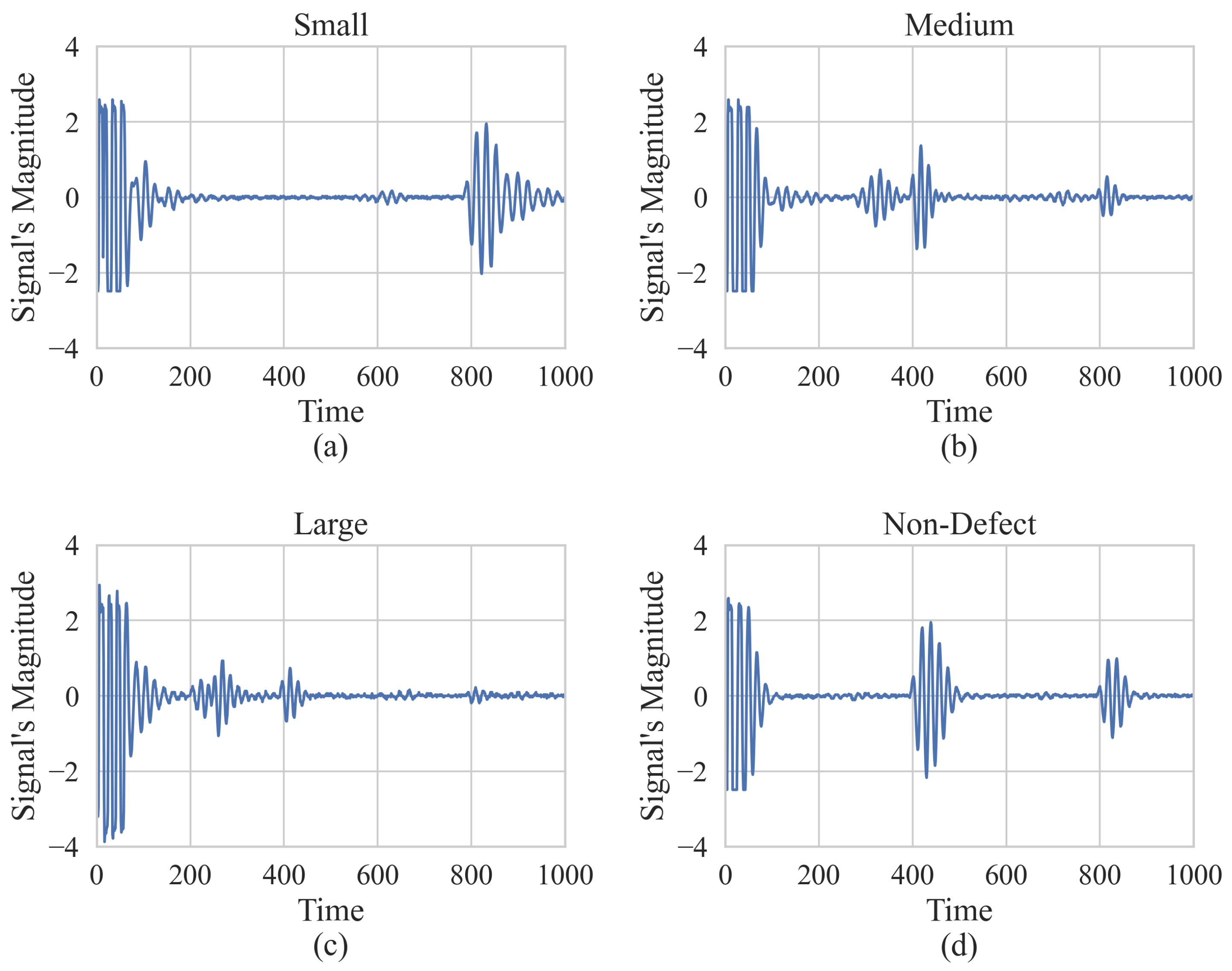
The presence of a defect results in additional echoes between the initial pulse and echo from the end of the material. Therefore, by comparing information associated with the additional echo in terms of magnitude with the initial and final pulse, we can have an estimation of the defect’s severity. The magnitude of the disturbance signal is proportional to the severity of the defect. Hence, the severity of the defect can be determined from the additional echo originating from it. In Figure 4, sending and receiving pulses are depicted for small defect, medium defect, large defect, and no defect conditions in Figure 4a, Figure 4b, Figure 4c, and Figure 4d, respectively.

The approach suggested in this paper involves creating a data frame containing the signal’s features (

Table 4. Time series data frame after data refinement.

Time Series	Time 1	Time 2	…	Time 999	Time 1000	Size
1	$-1.87$	1.47	…	$-0.07$	$-0.01$	Small
2	$-0.67$	1.93	…	0.01	$-0.01$	Medium
3	$-2.49$	0.03	…	$-0.01$	$-0.01$	Large
4	$-2.45$	0.87	…	0.03	0.01	Non-defect
. . . .	. . . .	. . . .	. . . .	. . . .	. . . .	. . . .
97	$-2.49$	$-0.03$	…	0.03	0.01	Small
98	$-2.49$	$-0.35$	…	0.01	0.03	Medium
99	$-2.37$	0.95	…	0.01	$-0.01$	Large
100	$-2.94$	$-0.192$	…	$-0.032$	$-0.032$	Non-defect

). Since each signal extracted from the oscilloscope comprises 1000 time points with their respective amplitude, the greatness of each signal throughout this 1000-point period can be considered as its feature, allowing for signal comparison. Thus, the resulting data frame contains 1000 columns representing time points as features, with each signal’s amplitude passed to the corresponding column, giving each signal its own value. The data frame is completed with one more column indicating the classification of each signal. Once completed, the resulting data frame can be seen in Table 3. Echo’s magnitude is box-plotted for each defect class shown in Figure 5.

In this study, five ML methods are utilized and compared to conduct classification analysis to estimate the size of the defects. Each ML method is run on two datasets. First, the ML methods are applied to the raw data obtained from experiments. Since there are one thousand data points, this could result in multiple features and lower accuracy. To address this, Principal Component Analysis (PCA) is used to effectively reduce the features and potentially obtain better accuracy. Therefore, an abbreviated data frame is obtained by applying PCA to the raw data, resulting in enhanced accuracy. This paper is notable for its innovative approach to extracting raw signals from laboratory experiments as the datasets are fitted to the ML methods in order to compare their performance. Following this, the data associated with the signals will be analyzed using the PCA method in order to determine the extent to which the performance can be improved.

2.3.1. Principal Component Analysis

A data frame may contain redundant features that may compromise the accuracy of the Ml methods. To address this issue, Principal Component Analysis (PCA) is commonly used to reduce the dimensionality of the data while maintaining the most relevant information [10,26]. PCA is known for its low noise sensitivity and high efficiency in smaller dimensions. Additionally, it is often applied to reduce the feature vector of laser ultrasonic signals [27]. In this study, since the proposed data frame contains 1000 features, applying PCA to reduce the feature dimensionality can lead to enhanced accuracy.

PCA is used to convert the original feature data group into a subspace by employing orthogonal transformations to eliminate irregularities in the raw data and project the original data from a high-dimensional to a low-dimensional space [28]. Let us consider a data frame where $x_i$ contributes as features, $y_i$ as label size classification, and T represents the vector transpose with respect to the mean $\overline{x}$.

$$COV\left(x\right)=\frac{1}{n}\sum _i^{i=n}\left(x_i-\overline{x}\right){\left(x_i-\overline{x}\right)}^T$$

(3)

The covariance matrix of $x_i$ features can be calculated to find the eigenvectors $m_i$ that correspond to the eigenvalues ${\lambda }_i$. Therefore, we can obtain both the eigenvectors matrix and the eigenvalues matrix:

$${\lambda }_i{m}_i=COV\left(x\right)m_i,i=1,2,\dots ,n$$

(4)

$$\begin{array}{cc}M=\left(m_i\right)& \\ A=diag\left({\lambda }_i\right)\end{array}$$

(5)

As a result, the largest eigenvalue d($d\le n$) can be chosen based on the cumulative contribution rate for reducing the feature dimensions:

$$\frac{{\sum }_{i=1}^d{\lambda }_i}{{\sum }_{i=1}^n{\lambda }_i}\times 100$$

(6)

As a result, the value of d can be determined based on the threshold parameter T. Then, the principal components of feature vectors with a lower dimension, determined using the h largest eigenvalues, can be obtained using the following method:

$${[m_1,m_1,m_1,\dots ,m_1]}^T\times x_i$$

(7)

2.3.2. ML Classification Methods

The supervised ML methods, including Decision Tree, Random Forest, Logistic Regression, K-Nearest neighbors, and Support vector machines, are widely used for classification challenges due to their outstanding superiority [29]. In this study, all five methods are compared against each other to conduct a classification analysis for quantifying the size of the defect. To ensure a fair assessment of computational efficiency across different models, a uniform environment was utilized. Python on Google Colab was the programming language employed for all machine learning processes. Moreover, the intuition and detail of each model are interpreted below [29]. Additionally, Grid Search was leveraged to obtain the parameters for each ML method in a manner resulting in the best performance.

Decision Tree

The regression process in this method involves dividing a dataset into smaller sub-datasets and developing a decision tree that is constructed incrementally using the data. The result is a decision tree that consists of decision nodes and leaf nodes.

Random Forest

It is an extension of bagging that introduces an additional level of randomness. Instead of using all predictors to split a node, a random subset of predictors is chosen to find the optimal split. The decision trees are constructed independently and combined to form a forest. This method is easy to use and requires only two parameters: the number of trees in the forest and the number of predictors considered at each node [30].

Logistic Regression

It is a reliable method for addressing binary classification problems. It utilizes a logistic function, which is an S-shaped curve that transforms any real-valued input into an output value between 0 and 1 (but never exactly at 0 or 1), to predict the probability of an outcome with only two possible values [31].

K Nearest Neighbors

This technique is valued for its simplicity, owing to factors such as ease of interpretation and quick calculation time. It involves storing available cases and classifying new cases based on their similarity to existing cases, which is determined using a measure, like distance. The object is classified by tallying the classification of its nearest neighbors and assigning it to the most common class. 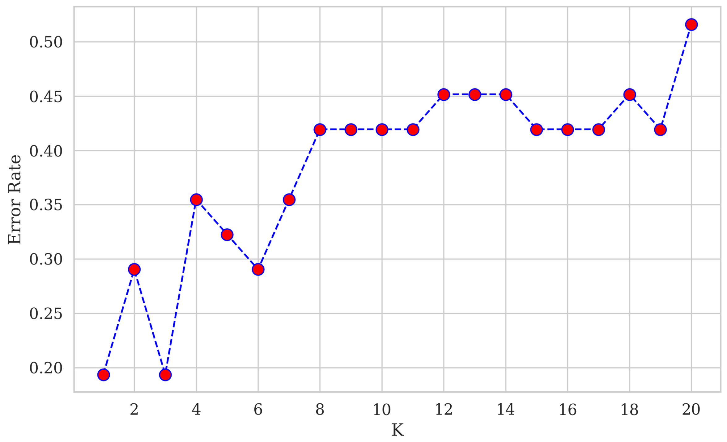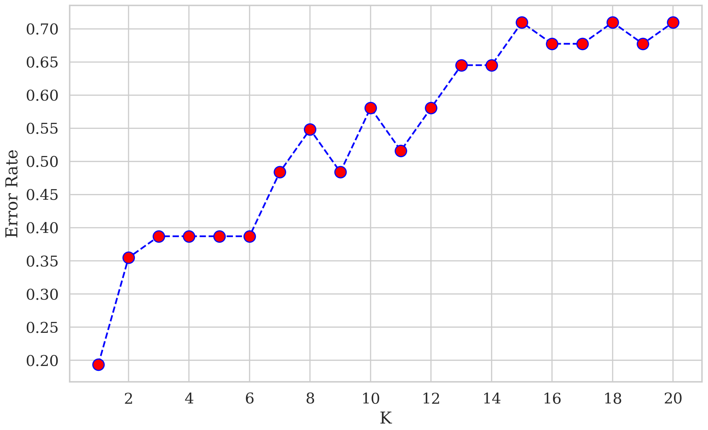This is performed by identifying the class with the highest similarity among the K nearest neighbors, of which the object is then assigned to that class [7]. As for choosing the most suitable value for K, we can plot our errors for each K and obtain the K value with the minimum error rate. The error rate versus K values is depicted in Figure 6 (before applying PCA) and Figure 7 (after applying PCA).

Support Vector Machines

The SVM algorithm has proven to be a highly effective tool for solving binary classification problems in practical applications. Research has demonstrated that SVMs outperform other supervised learning techniques in terms of classification accuracy and generalization performance [8]. In recent years, SVMs have emerged as one of the most widely used classification methods due to their strong theoretical foundations and superior generalization ability. Their popularity has increased significantly as they have demonstrated impressive performance in various real-world applications.

The primary objective of SVM is to effectively separate multiple classes in the training dataset using a surface that maximizes the margin between them. This, in turn, maximizes the generalization ability of the model. This aligns with the Structural Risk Minimization principle (SRM), which aims to minimize the generalization error bound of a model rather than simply minimizing the mean squared error on the training dataset, as is typically performed using empirical risk minimization methods.

By prioritizing generalization over minimizing the training error, SVM can produce more reliable and accurate predictions on new, unseen data [9].

3. Results

3.1. Defect Localization

Focusing on sample A as a case study to demonstrate the method for defect localization, the transducer was placed on the surface of the sample. The method highlighted in the methodology section above was then applied to observe the waveform on the oscilloscope, which can be seen in Figure 3.

An extra echo was observed before the echo, indicating the end of sample B (as shown in Figure 8b). To determine the time for the defect echo and the end-of-material echo, a vertical cursor was used to track their respective times. The defect echo was received 609 ns after the initial signal, while the end-of-material echo was received 1378 ns later. By using the time values obtained along with the sound velocity for stainless steel (5800 m/s). These values are plugged into Equation (2) to locate the defect.

$$d=\frac{vt}{2}$$

$$v=5800\mathrm{m}/\mathrm{s}=5,800,000\mathrm{mm}/\mathrm{s};t=609\mathrm{ns}$$

$$d_{defect}=\frac{5,800,000\times (609\times {10}^{-9})}{2}=1.7661\mathrm{mm}$$

$$\begin{array}{c}\hfill d_{end-of-material}=\frac{5,800,000\times (1378\times {10}^{-9})}{2}=3.9962\mathrm{mm}\\ \hfill =4\mathrm{mm}\end{array}$$

The calculations indicate that the defect is located near the center of sample B. As the thickness of the sample is 4 mm and the echo indicating the end of the material corresponds to this value, it proves the reliability of this method. The ultrasonic piezoelectric transducer is not only helpful in detecting defects but also in estimating the distance of the defect from the surface of the sample. The use of a couplant is necessary to allow a significant amount of waves to pass into the material being tested. The test conducted on sample A was successful.

3.2. Defect Severity

3.2.1. Feature Reduction

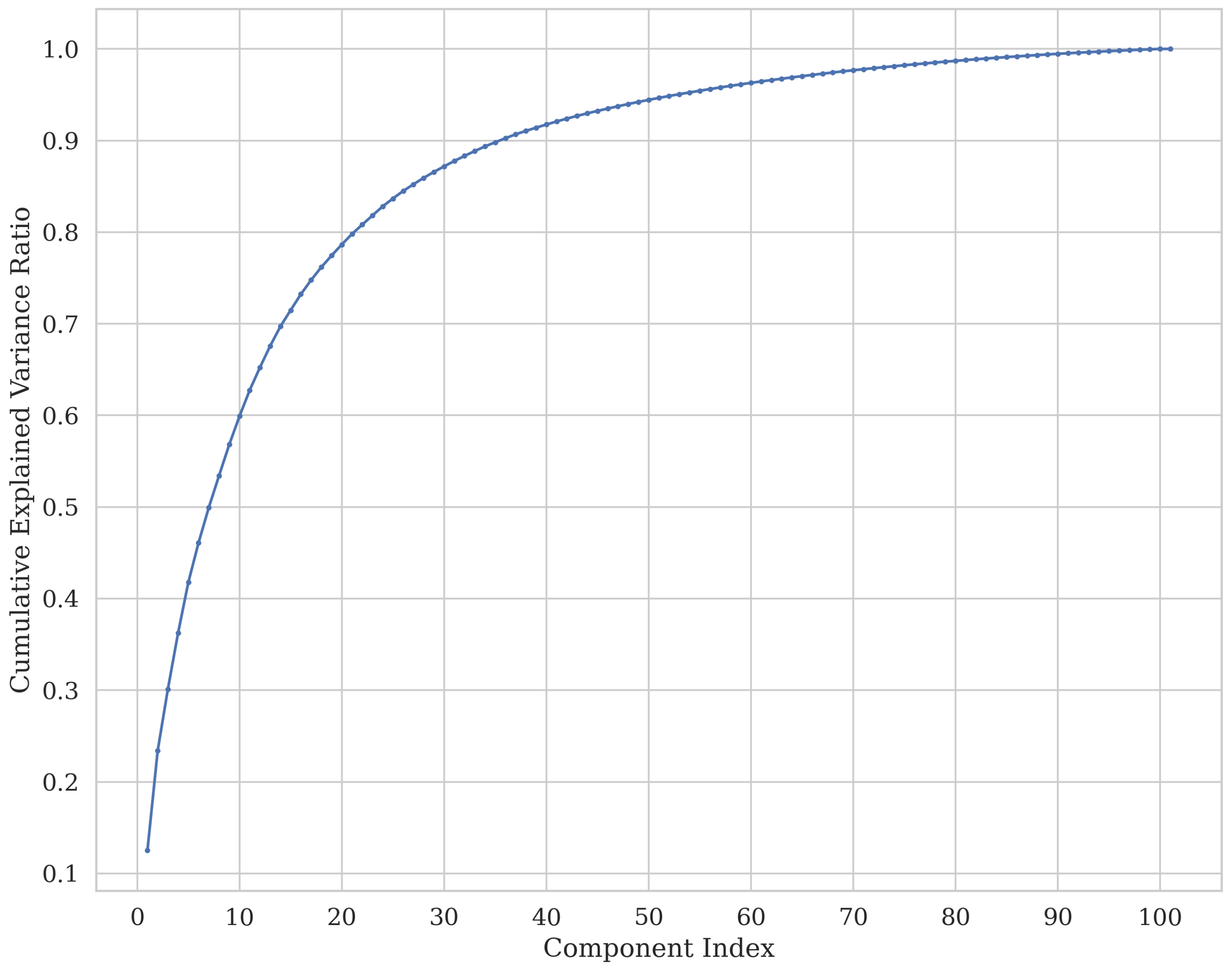
To improve the performance of ML models, feature reduction is implemented to mitigate the dimensionality of the feature datasets. Superfluous feature datasets can result in reduced accuracy of the model [10]. Therefore, PCA is implemented to remove redundant features and retain only those that have a profound impact on the determination of results. We may ascertain the number of components necessary to enhance the model performance by referring to Figure 9, which displays the cumulative explained variance ratio as a function of the number of components. Consequently, we were able to keep 90% of the variance by reducing the number of components to 36. As we can see in Figure 4, since only the signal information associated with the part where the defect is located is important for us, we can neglect the signal information showing the beginning and ending, which leads to better accuracy for each ML model as well as a faster training process.

3.2.2. Models’ Training and Testing

In order to assess the effectiveness of the PCA algorithm, the following datasets were used. The selected ML models were trained with the data both with and without PCA treatment. It is important to reduce bias resulting from random data selection to ensure robust evaluation results. Therefore, five-fold cross-validation was used throughout this study, with 70% and 80% of the total 100 samples randomly selected for training the ML models, and the remaining 30% and 20% of the data dedicated to evaluating the models [11,32].

3.2.3. Results of ML Models’ Assessment

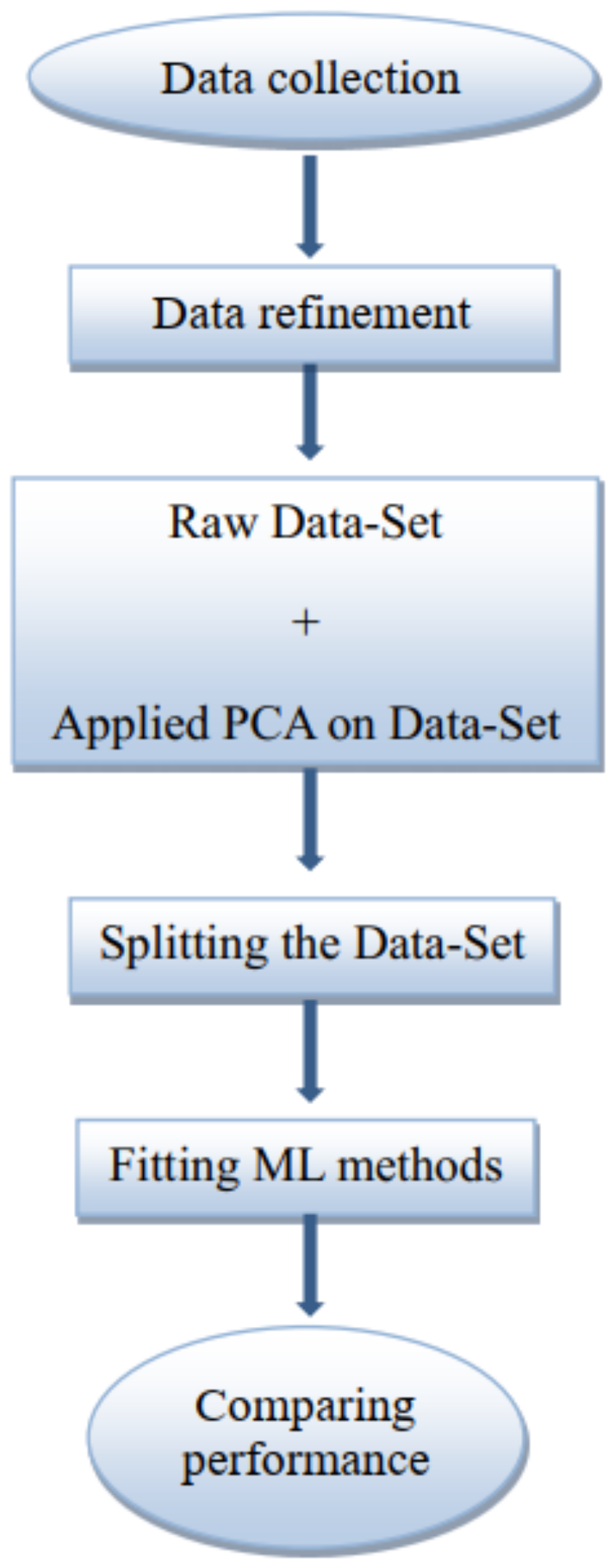
As mentioned in the methodology, a comparison of the performance of ML methods is conducted using both raw data and PCA-processed data. To achieve this, as shown in

Table 5. ML methods performed and comparing their accuracy, precision, recall, and F1 Score as data is divided and fitted by common manners.

Reports/Methods		By 20 vs. 80				By 30 vs. 70				By five folds
		Accuracy	Precision	Recalls	F1-Scores	Accuracy	Precision	Recalls	F1-Scores	Accuracy	Precision	Recalls	F1-Scores
Raw Data	SVM	75	78	76	74	75	78	76	74	78	80	73	73
	DT	75	77	76	74	74	77	76	74	72	75	69	69
	RF	89	91	90	89	88	90	89	88	89	87	87	86
	KNN	91	92	92	91	88	90	89	89	91	93	92	91
	LR	87	89	88	87	85	87	86	85	89	91	91	90
PCA Reduced Feature	SVM	98	98	98	98	97	97	98	97	99	99	99	99
	DT	96	97	97	97	96	97	97	96	98	98	98	98
	RF	96	97	97	97	95	96	96	96	96	97	96	96
	KNN	89	92	90	89	85	89	86	86	87	92	87	87
	LR	97	97	97	97	96	97	97	96	97	98	97	97

All values are in percentage.

, the correlation metric coefficients (Accuracy, Precision, Recall, and F1 score) were calculated from the datasets both with and without PCA treatment [33]. Although KNN is the only ML method that does not show improvement, all of the other methods do. Additionally, based on the performance of the SVM model, it is evident that it possesses the highest accuracy among all the methods. The process of defect detection and classification is summarized in a flowchart shown in Figure 10.

4. Discussion

While it is true that both ultrasonic testing and traditional Machine Learning (ML) methods have established themselves as valuable tools in the realm of non-destructive testing (NDT), the novelty of this study lies in their integration within the specific context of 3D-printed metal structures. The intersection of these two well-established domains creates a unique synergy that offers distinct advantages over existing approaches.

Firstly, the novelty of this research stems from its emphasis on the application of ultrasonic testing to 3D-printed metal components. While ultrasonic testing is not new to NDT, its adaptation to the intricate and evolving landscape of additive manufacturing presents a fresh challenge. The varying material properties, geometric complexities, and layer-by-layer fabrication process of 3D printing introduce unique acoustic characteristics that require tailored testing methods. This study investigates how ultrasonic piezoelectric transducers can be optimized and customized for the specific requirements of 3D-printed metal structures, addressing a critical gap in the literature.

Secondly, the innovation lies in the comparative analysis of Machine Learning (ML) methods in tandem with traditional NDT techniques for defect classification in AM. While ML has made significant inroads in various fields, its application within AM, particularly for defect classification, remains an evolving frontier. This research goes beyond simply applying ML to the NDT data; it delves into the comparative performance of five prominent ML methods within the specific context of AM. By systematically evaluating Decision Trees, Random Forests, Logistic Regressions, K-Nearest Neighbors, and Support Vector Machines, this study offers valuable insights into which ML algorithms are best suited for AM defect classification.

In essence, the novelty of this study lies in its tailored approach to addressing the unique challenges posed by 3D-printed metal structures via the integration of ultrasonic testing and ML, ultimately paving the way for more reliable and efficient quality control in additive manufacturing.

5. Conclusions

Testing is crucial in identifying internal defects such as voids and holes in materials before they are put into service. Failure to detect a defect and accurately quantify its severity can result in accidents or failures during service. For testing purposes, two samples, each with similar defects, were used. Ultrasonic testing was performed on samples A and B, where internal defects were accurately detected, and their locations were estimated with precision. The method was successful in detecting the presence of a defect and determining its location within the structure from the returned signal. The location could also be visibly estimated on the oscilloscope.

The size of the defect is a crucial part of defect detection. The presence of a defect creates additional echoes, of which the magnitude of the defect can be determined by examining these echoes. Therefore, ML methods can be used to estimate the size of the defect by analyzing the amplitude values of the additional echoes. In this study, 100 sample signals were utilized, with 25 samples for each size classification: Small, Medium, Large, and non-defect. All data associated with the samples were obtained via the experimental procedure. The five ML models were compared—Decision Tree, Random Forest, Logistic Regression, K-Nearest Neighbors, and Support Vector Machines, to determine the size of the defects. Based on the results, SVM shows better performance, holding a 98%, 97%, and 99% accuracy for three data distribution approaches, including 70% and 80% of the total samples as training samples along with a five-fold cross-validation test, followed by TD, which shows a 98% accuracy as its highest accuracy, and LR, standing in the third place holding a 97% accuracy. Moreover, as illustrated in Table 5, significant improvements are evident in all of the methods when PCA is applied to the data supplied to the machine learning methods. Specifically, we can see around a 20% improvement in accuracy when PCA is applied to the datasets that are analyzed using methods such as SVM and DT. The prominent trend in Table 5, which illustrates the enhancement that k-fold cross-validation provides to all methods, indicates that this approach to data distribution is superior to the traditional training datasets of 70% and 80%. We also used PCA analysis to reduce redundant features, resulting in enhanced accuracy. The results showed that SVM had the best performance among all models. Although ML offers distinct benefits, there are strict application requirements. For manufacturing systems, the tiny datasets that are normally accessible lead to overfitting models, which result in low fault detection accuracy. A significant obstacle to the practical application of ML in defect identification is the absence of accurate, thorough, and easily available databases for various materials, designs, and printing techniques.

The main contributions of this study include:

• Successful Ultrasonic Testing: Implemented ultrasonic testing on different samples, accurately detecting internal defects and precisely estimating their locations within the structure.
• ML-Based Size Estimation: Used ML methods, including SVM with a 98–99% accuracy, for defect size estimation by analyzing amplitude values in 100 sample signals.
• Enhanced Accuracy with PCA: Applied PCA to improve accuracy, particularly with SVM showing significant improvement, and emphasized the need for comprehensive databases in ML applications for effective defect identification.

In light of our findings, future endeavors will focus on diverse materials, varying 3D printing shape, and smaller defect sizes, aiming for more precise outcomes. This extended research will contribute significantly to a deeper understanding of the impacts of the above-mentioned parameters on defect detection and potentially unlock new avenues for innovation and application in non-destructive testing.

References

- Savini, A.; Savini, G. A short history of 3D printing, a technological revolution just started. In Proceedings of the 2015 ICOHTEC/IEEE International History of High-Technologies and Their Socio-Cultural Contexts Conference (HISTELCON), Tel-Aviv, Israel, 18–19 August 2015; pp. 1–8. [Google Scholar] [CrossRef]
- Rahimizadeh, A.; Kalman, J.; Fayazbakhsh, K.; Lessard, L. Mechanical and thermal study of 3D printing composite filaments from wind turbine waste. Polym. Compos. 2021, 42, 2305–2316. [Google Scholar] [CrossRef]
- Sam-Daliri, O.; Ghabezi, P.; Steinbach, J.; Flanagan, T.; Finnegan, W.; Mitchell, S.; Harrison, N. Experimental study on mechanical properties of material extrusion additive manufactured parts from recycled glass fibre-reinforced polypropylene composite. Compos. Sci. Technol. 2023, 241, 110125. [Google Scholar] [CrossRef]
- Rahimizadeh, A.; Kalman, J.; Fayazbakhsh, K.; Lessard, L. Recycling of fiberglass wind turbine blades into reinforced filaments for use in Additive Manufacturing. Compos. Part B Eng. 2019, 175, 107101. [Google Scholar] [CrossRef]
- Pereira, T.; Potgieter, J.; Kennedy, J. Development of Quality Management Strategies for 3D Printing Testing Methods—A Review. In Proceedings of the 2017 4th Asia-Pacific World Congress on Computer Science and Engineering (APWC on CSE), Mana Island, Fiji, 11–13 December 2017; pp. 224–231. [Google Scholar] [CrossRef]
- Dwivedi, S.; Vishwakarma, M.; Soni, A. Advances and Researches on Non Destructive Testing: A Review. Mater. Today Proc. 2018, 5, 3690–3698. [Google Scholar] [CrossRef]
- Bicego, M.; Loog, M. Weighted K-nearest neighbor revisited. In Proceedings of the 2016 23rd International Conference on Pattern Recognition (ICPR), Cancun, Mexico, 4–8 December 2016; IEEE: Piscataway, NJ, USA, 2016; pp. 1642–1647. [Google Scholar]
- Sun, B.Y.; Huang, D.S.; Fang, H.T. Lidar signal denoising using least-squares support vector machine. IEEE Signal Process. Lett. 2005, 12, 101–104. [Google Scholar]
- Cervantes, J.; Garcia-Lamont, F.; Rodríguez-Mazahua, L.; Lopez, A. A comprehensive survey on support vector machine classification: Applications, challenges and trends. Neurocomputing 2020, 408, 189–215. [Google Scholar] [CrossRef]
- Su, L.; Shi, T.; Liu, Z.; Zhou, H.; Du, L.; Liao, G. Nondestructive diagnosis of flip chips based on vibration analysis using PCA-RBF. Mech. Syst. Signal Process. 2017, 85, 849–856. [Google Scholar] [CrossRef]
- Wong, T.T.; Yeh, P.Y. Reliable accuracy estimates from k-fold cross validation. IEEE Trans. Knowl. Data Eng. 2019, 32, 1586–1594. [Google Scholar] [CrossRef]
- Luo, H.; Sun, X.; Xu, L.; He, W.; Liang, X. A review on stress determination and control in metal-based additive manufacturing. Theor. Appl. Mech. Lett. 2022, 13, 100396. [Google Scholar] [CrossRef]
- 3DEXPERIENCE Platform. Available online: https://make.3dexperience.3ds.com/materials/metal-materials-for-3d-printing-processes (accessed on 7 November 2022).
- Beemaraj, R.K. Optimization of CNC machining parameters for surface roughness in turning of Aluminium 6063 T6 with response surface methodology. Int. J. Mech. Eng. 2018, 2, 23. [Google Scholar]
- Shepheard, S. The Complete Aluminum 3D Printing Guide. 2020. Available online: https://www.3dsourced.com/3d-printer-materials/3d-printing-aluminum-guide/ (accessed on 7 November 2022).
- Stainless Steel Material for 3D Printing-Ultimate Guide. 2021. Available online: https://pick3dprinter.com/3d-printing-stainless-steel/ (accessed on 7 November 2022).
- Pereira, T.; Potgieter, J.; Kennedy, J. A fundamental study of 3D printing testing methods for the development of new quality management strategies. In Proceedings of the 2017 24th International Conference on Mechatronics and Machine Vision in Practice (M2VIP), Auckland, New Zealand, 21–23 November 2017; pp. 1–6. [Google Scholar] [CrossRef]
- Pierce, J.; Crane, N. Preliminary Nondestructive Testing Analysis on 3D Printed Structure Using Pulsed Thermography. In Proceedings of the ASME International Mechanical Engineering Congress and Exposition, Tampa, FL, USA, 3–9 November 2017; p. V008T10A083. [Google Scholar] [CrossRef]
- Elsaadouny, M.; Barowski, J.; Jebramcik, J.; Rolfes, I. Millimeter Wave SAR Imaging for the Non-Destructive Testing of 3D-printed Samples. In Proceedings of the 2019 International Conference on Electromagnetics in Advanced Applications (ICEAA), Granada, Spain, 9–13 September 2019; pp. 1283–1285. [Google Scholar] [CrossRef]
- Makagonov, N.; Blinova, E.; Bezukladnikov, I. Development of visual inspection systems for 3D printing. In Proceedings of the 2017 IEEE Conference of Russian Young Researchers in Electrical and Electronic Engineering (EIConRus), St. Petersburg and Moscow, Russia, 1–3 February 2017; pp. 1463–1465. [Google Scholar] [CrossRef]
- Cui, S.; Ling, P.; Zhu, H.; Keener, H.M. Plant pest detection using an artificial nose system: A review. Sensors 2018, 18, 378. [Google Scholar] [CrossRef]
- Pyle, R.J.; Bevan, R.L.; Hughes, R.R.; Rachev, R.K.; Ali, A.A.S.; Wilcox, P.D. Deep learning for ultrasonic crack characterization in NDE. IEEE Trans. Ultrason. Ferroelectr. Freq. Control 2020, 68, 1854–1865. [Google Scholar] [CrossRef]
- Yang, J.; Li, S.; Wang, Z.; Dong, H.; Wang, J.; Tang, S. Using deep learning to detect defects in manufacturing: A comprehensive survey and current challenges. Materials 2020, 13, 5755. [Google Scholar] [CrossRef]
- Chen, G.H.; Zhang, X.M.; Xie, C.H.; He, X.B. Intelligent recognition of crack depth in ultrasonic testing. Huanan Ligong Daxue Xuebao/J. South China Univ. Technol. (Nat. Sci.) 2005, 33, 1–5. [Google Scholar]
- Abdullah, M.; Zainal Abidin, M.F.; Elmi, A.; Mahmod, M.F. Feature Analysis Thru Image Recognition of C-Scan Image for Composite Laminated Materials. In Proceedings of the 27th International Invention & Innovation Exhibition, Kuala Lumpur, Malaysia, 12–14 May 2016. [Google Scholar]
- Karamizadeh, S.; Abdullah, S.M.; Manaf, A.A.; Zamani, M.; Hooman, A. An overview of principal component analysis. J. Signal Inf. Process. 2013, 4, 173. [Google Scholar] [CrossRef]
- Li, K.; Sui, H.; Dong, X.; Guo, L.; Gao, H. Intelligent Evaluation of Crack detection with Laser Ultrasonic technique. In Proceedings of the IOP Conference Series: Earth and Environmental Science, Changchun, China, 21–23 August 2020; IOP Publishing: Bristol, UK, 2020; Volume 514, p. 022014. [Google Scholar]
- Lv, G.; Guo, S.; Chen, D.; Feng, H.; Zhang, K.; Liu, Y.; Feng, W. Laser ultrasonics and machine learning for automatic defect detection in metallic components. NDT E Int. 2023, 133, 102752. [Google Scholar] [CrossRef]
- Choudhary, R.; Gianey, H.K. Comprehensive review on supervised machine learning algorithms. In Proceedings of the 2017 International Conference on Machine Learning and Data Science (MLDS), Noida, India, 14–15 December 2017; IEEE: Piscataway, NJ, USA, 2017; pp. 37–43. [Google Scholar]
- Liaw, A.; Wiener, M. Classification and regression by randomForest. R News 2002, 2, 18–22. [Google Scholar]
- Brownlee, J. Logistic Regression for Machine Learning-Machine Learning Mastery. Machine Learning Mastery. 2016. Available online: http://machinelearningmastery.com/logistic-regression-for-machine-learning/ (accessed on 12 August 2017).
- Buntine, W.; Niblett, T. A further comparison of splitting rules for decision-tree induction. Mach. Learn. 1992, 8, 75–85. [Google Scholar] [CrossRef]
- Goutte, C.; Gaussier, E. A probabilistic interpretation of precision, recall and F-score, with implication for evaluation. In Proceedings of the Advances in Information Retrieval: 27th European Conference on IR Research, ECIR 2005, Santiago de Compostela, Spain, 21–23 March 2005; Proceedings 27. Springer: Berlin/Heidelberg, Germany, 2005; pp. 345–359. [Google Scholar]
Figure 1.
Schematic illustration of the test setup, showing the flow from the transducer to the waveform on the oscilloscope.
Figure 2.
A-scan technique for data visualization showing the magnitude of the signal against time.
Figure 3.
Setup comprising of ultrasonic transducer, pulser–receiver, and oscilloscope.
Figure 4.
Sample (a) Small defect, (b) Medium defect, (c) Large defect, and (d) No defect signals extracted from oscilloscope for four different defect sizes.
Figure 5.
Box plots showing the magnitude of defect echoes for each size classification.
Figure 6.
Plotting the error rate against K values to select the best value of K.
Figure 7.
Plotting the error rate against K values to select the best value of K after applying PCA.
Figure 8.
Output waveform for test on sample A (a) showing the initial pulse and the echo from the end of material; (b) showing an additional echo signifying the presence of an internal defect within the structure.
Figure 9.
Number of principal components required to reach a 90% cut-off threshold.
Figure 10.
Flow chart depicting the procedure of how raw data from the oscilloscope proceed, making them applicable and fitted to ML methods in order to conduct comparison.