Article

Design and Implementation of a Recursive Feedforward-Based Virtual Reference Feedback Tuning (VRFT) Controller for Temperature Uniformity Control Applications

1
Electronic Engineering, Pontifical Bolivarian University, Medellín 050031, Colombia
2
School of Engineering, University of California, Merced, CA 95343, USA
*
Author to whom correspondence should be addressed.
Machines 2023, 11(10), 975; https://doi.org/10.3390/machines11100975
Submission received: 26 September 2023 / Revised: 15 October 2023 / Accepted: 17 October 2023 / Published: 20 October 2023
(This article belongs to the Special Issue New Trends in Robotics and Automation)

Abstract

:
Data-driven controller synthesis methods use input/output information to find the coefficients of a proposed control architecture. Virtual Reference Feedback Tuning (VRFT) is one of the most popular frameworks due to its simplicity and one-shoot synthesis style based on open-loop system response for classic regulators such as PI or PID. This paper presents a recursive VRFT framework to extend VRFT into high-order controllers with more complex structures. The framework first defines a reference model and controller structure, then uses the open-loop data to compute the virtual reference and error signals, and, finally, uses these to find the controller parameters via an optimization algorithm. Likewise, the recursive VRFT controller performance is improved by adding a model-based feedforward loop to improve reference signal tracking. The recursive method is tested to design a temperature uniformity control system. The obtained results show that the recursive VRFT with a feedforward improves the system response while allowing more complex controller synthesis.

1. Introduction

Model-based control methods cover an important part of control systems design. These are supported by mathematical process models for the design and synthesis of a closed-loop controller [1]. However, obtaining an acceptable process model can be challenging in processes with uncertainty and non-linear behavior, compromising the system’s stability and performance [1,2,3,4]. This is especially relevant for processes that face variable environments that may require not only an acceptable model but also a constant parameter adaptation using optimization algorithms or adaptive control methodologies, such as [5,6,7,8,9,10,11]. Thus, the interest in data-driven control methods has been increasingly motivated by the increasing availability of process data given new technologies such as IoT, edge computing, or cheap sensing [12]. Some of these methods include Iterative Feedback Tuning [13], dynamic mode decomposition [14], Iterative Learning Control [15], extremum seeking [16], model-free adaptive control [17], unfalsified control [18], and simultaneous perturbation stochastic approximation [19].
One of the most studied data-driven control methods is the Virtual Reference Feedback Tuning (VRFT). It uses input–output data from a process to generate a virtual reference signal based on a desired reference model to find the optimal parameters that minimize the difference with the desired behavior [20,21].
Some applications of VRFT include motion controls, power electronics, or process control. For example, [22] employs a dual VRFT controller tuning method for velocity ripple compensation on a motor system. In [23], VRFT is employed to find the compensator for several DC–DC power converters with non-minimum phase (NMP) behavior as buck, boost, and buck–boost configurations with a reference model that compensates for the NMP zero. Likewise, [24] presents the use of VRFT on a cooperative control system with Neuroendocrine Ultrashort Feedback Controllers. Moreover, VRFT can be employed on multiple input multiple output (MIMO) configurations by defining a multivariable reference model [25] or combined with the internal model control (IMC) design method for dual temperature control [26].
In these applications, the synthesis process of VRFT follows the standard framework proposed by [20] following standard controller architectures such as PI and PID, and the model reference selection is based on prior knowledge of the system response. However, sometimes, the controller response has differences regarding its desired response. This can be explained by the fact that there are no criteria for reference model selection within the controller design method that ensure adequate closed-loop system performance.
This paper presents the design of a data-driven controller based on the Virtual Reference Feedback Tuning (VRFT) framework [3] to improve the setpoint tracking response of uniform temperature control systems.
Unlike other VRFT approaches, this work first generates the virtual error signal using the system’s data-driven response with the reference model. Then, a compensator transfer function is selected (e.g., first-order, second-order, high-order), and parameters are determined through an optimization algorithm using the virtual error as input and control action as output signals. The controller synthesis process evaluates several reference model structures to select a suitable one that minimizes the system’s energy consumption and steady-state error and allows a lower-order system implementation. Likewise, the proposed controller uses adaptive feedforward compensation based on the desired reference system model to improve the closed-loop system response based on the error between the reference model and system output. The proposed VRFT controller is tested for the temperature uniformity control of a Peltier thermoelectric system in simulation and experimentally using hardware in the loop configuration. The VRFT controller is evaluated against the classic PI controller tuned via pole IMC and Skogestad IMC (SIMC) [27].
The contributions of this paper are:
  • Extending the VRFT framework for synthesizing different control structures through an optimization process using the virtual error signal obtained only from the system data.
  • Present a method to assess reference models for VRFT controller design and different compensator architectures.
  • Add a feedforward compensation to the system using the VRFT reference model to improve closed-loop response in setpoint tracking tasks.
The main benefit of the proposed algorithm is the recursive solution of the VRFT control problem, which can be extended into controllers with fixed complex structures, such as high-order compensators or non-linear controllers in SISO and MIMO configurations that include feedforward capabilities. Thus, the controller parameters are synthesized using an optimization algorithm using the virtual error that minimizes the control action and tracking error based on a desired reference model.
The manuscript is structured as follows. Section 2 introduces the foundations of VRFT controller design. Section 3 shows the recursive framework used to obtain the virtual error signal, the optimization process for VRFT synthesis, and the feedforward compensation scheme based on the reference model. Section 4 shows a case study corresponding to the temperature uniformity control system and its modeling using multiphysics simulation tools, the VRFT controller synthesis, feedforward design, and its validation in the simulation environment. Section 5 shows the experimental validation of the VRFT controller on the temperature uniformity control system. Finally, our conclusions and possibilities for future work are presented.

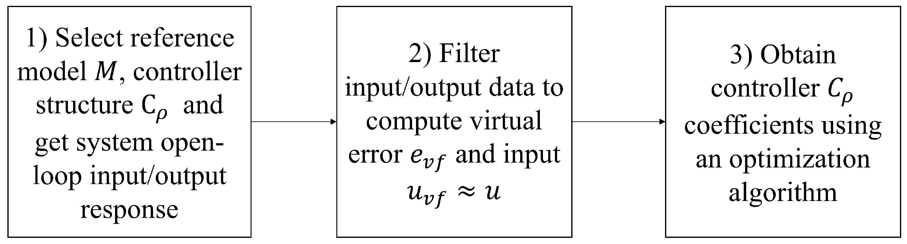
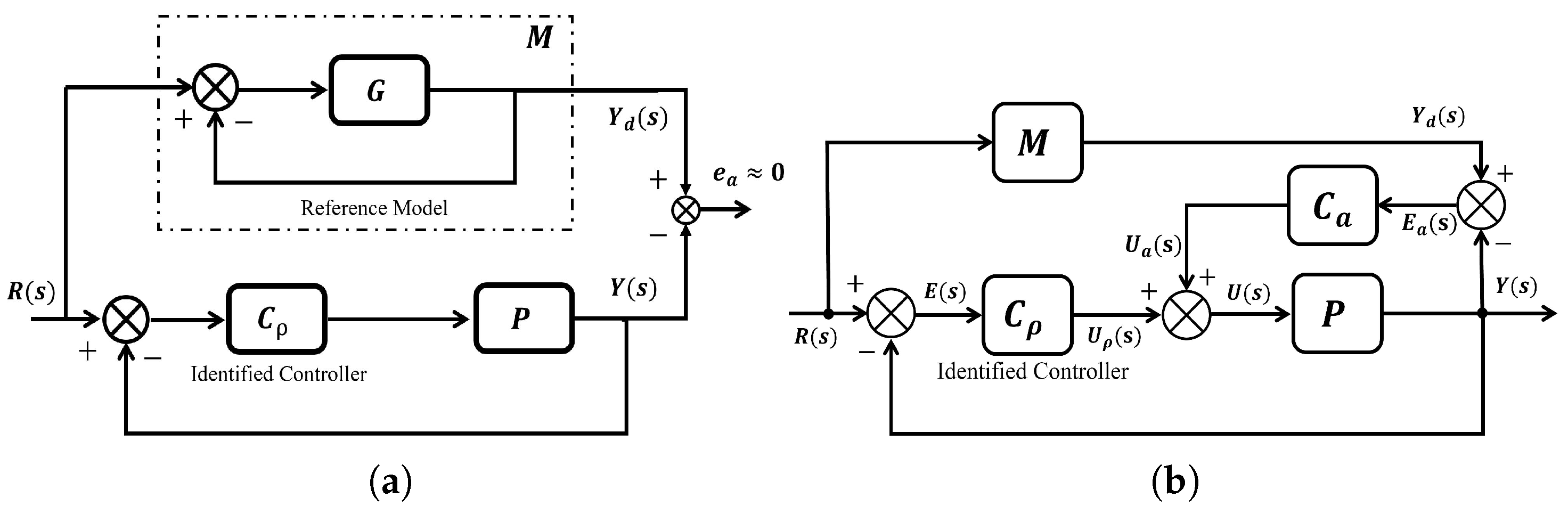
2. VRFT Control Framework

The VRFT framework is shown in Figure 1. Initially, an input–output u ( t ) , y ( t ) open-loop response dataset of the system P is obtained, and a reference model M is defined to establish the system’s desired behavior. So, using the inverse reference model M 1 , the virtual reference r v ( r ) is created to compute the virtual error e v ( t ) . Thus, after selecting a structure for the controller C ρ , its coefficients are determined using the virtual error signal e v ( t ) to make the virtual control action u v ( t ) closer to the real system’s control action u ( t ) [28,29]. During the data acquisition process, it is important that the input signal u ( t ) satisfies the persistent excitation conditions to ensure a representative output y ( t ) in terms of system identification. Likewise, filtering y ( t ) is crucial for calculation of the virtual error e v ( t ) and the controller’s synthesis quality [21,28]. Thus, using the filtered version of the input–output signals u f ( t ) = u ( t ) F ( t ) y y f ( t ) = y ( t ) F ( t ) , where F ( t ) is the filter transfer function, the virtual reference signals r v f and e v f can be computed as (1)
r v f ( t ) = y f ( t ) M 1 , e v f ( t ) = r v f ( t ) y f ( t ) .
So, using the filtered signals [ e v f ( t ) , u f ( t ) ] , the parameters of the selected C ρ can be obtained by minimizing (2), where N is the total amount of data samples and θ is the vector of controller parameters.
J V R = lim N t = 1 N ( u f ( t ) C ρ ( z ; θ ) e v f ( t ) ) 2 .
Assuming that C ρ ( z ; θ ) is in the discrete domain z and is in the form C ρ ( z ; θ ) = β ( z ) θ , (2) can be rewritten as (3)
J V R = lim N t = 1 N ( u f ( t ) φ f T θ ) ) 2 φ f = β ( z ) e v f ( t ) .
Thus, (3) can be rewritten as a least squares problem, defined as (4), where θ ^ N is the estimated controller’s parameters’ vector.
θ ^ N = ( t = 1 N φ f ( t ) φ f T ( t ) ) 1 t = 1 N φ f ( t ) u f ( t ) .
It is important to notice that for standard controller structures, such as PI, PID, or PD, the VRFT problem can be straightforwardly expressed using (3) and (4). However, for more complex architectures, such as high-order transfer function-based or non-linear controllers, expressing the VRFT problem is harder. Therefore, this paper proposes solving (3) by using standard optimization procedures, leveraging the virtual error and reference signals for controller synthesis.

3. Recursive VRFT Controller Synthesis

The procedure to perform a recursive VRFT controller synthesis is shown in Figure 2. The first step defines the reference model M and the controller structure C ρ and collects the input–output data of the open-loop stable process.
In the second step, the input–output data are filtered to compute the reference signal’s E v using M. This procedure is illustrated on Figure 3. According to [21,28], the virtual error E v can be computed using Y ( s ) and the inverse reference model M 1 , as shown in Figure 3a, which can be simplified using the equivalent reference system G 1 shown in Figure 3b. Thus, M and G can be related in the frequency domain as (5).
M ( s ) = G ( s ) 1 + G ( s ) .
Likewise, (1) can be rewritten in the frequency domain as (6) and (7)
R v ( s ) = Y ( s ) M 1 ( s ) ,
E v ( s ) = R v ( s ) Y ( s ) .
Replacing (6) with (7), the virtual error in terms of M is given by (8)
E v ( s ) = Y ( s ) M 1 ( s ) Y ( s ) = Y ( s ) [ M 1 ( s ) 1 ] .
Now, substituting (5) in (8), the virtual error E v is expressed in terms of G ( s ) by (9), as shown in Figure 3b.
E v ( s ) = Y ( s ) 1 + G ( s ) G ( s ) 1 = Y ( s ) G 1 ( s ) .
Finally, in the third step, the coefficients of the controller C ρ can be calculated using an optimization algorithm using e v f and u v f as input/output signals, respectively. In this manuscript, the optimization stage is performed using the Matlab system identification toolbox in order to synthesize complex high-order controllers rather than classic PI or PID regulators.

Feedforward VRFT-SISO Controller Recursive Synthesis

As can be observed in Figure 4a, if the controller is ideal, it means C ρ = C i d e a l = G / P , and the error between the desired response of the system y d ( t ) and the current one y ( t ) is zero. However, the obtained controller C ρ is not ideal in almost all the cases, making e a 0 , showing a difference between the desired and actual system response. For this reason, the Feedforward VRFT-SISO controller shown in Figure 4b can be implemented to account for this mismatching. As can be observed, it uses the error signal E a ( s ) = Y d ( s ) Y ( s ) multiplied by C a ( s ) to produce an additional correction U a ( s ) to the control action U ( s ) to minimize the difference between the desired and actual process response. To analyze the controller response, the system response is computed as (10):
Y ( s ) = [ E ( s ) C ρ ( s ) + E a ( s ) C a ( s ) ] P ( s ) = [ [ R ( s ) Y ( s ) ] C ρ ( s ) [ Y d ( s ) Y ( s ) ] C a ( s ) ] P ( s ) ,
replacing Y d ( s ) = R ( s ) M in (10),
Y ( s ) [ 1 + P ( s ) [ C ρ ( s ) + C a ( s ) ] ] = R ( s ) [ C ρ ( s ) + M ( s ) C a ( s ) ] P ( s ) .
So, the system’s transfer function is given by (12)
Y ( s ) R ( s ) = P ( s ) [ C ρ ( s ) + M ( s ) C a ( s ) ] 1 + P ( s ) [ C ρ ( s ) + C a ( s ) ] .
Replacing C a ( s ) = k · C ρ ( s ) and (5) in (12), where k is a proportional gain, the closed-loop response is given as (13):
Y ( s ) R ( s ) = P ( s ) C ρ ( s ) [ 1 + ( k + 1 ) G ( s ) ] [ 1 + G ( s ) ] [ 1 + P ( s ) C ρ ( s ) ( k + 1 ) ] .
If the controller is ideal, C ρ ( s ) = C i d e a l ( s ) = G ( s ) / P ( s ) , and the feedforward will not affect the controller performance. However, if C ρ (s) is not ideal, the feedforward improves the process response. The effect will be more noticiable for a value of k that makes G ( s ) [ k + 1 ] 1 , so (13) can be approximated as (14).
Y ( s ) R ( s ) P ( s ) C ρ ( s ) [ G ( s ) ( k + 1 ) ] [ 1 + G ( s ) ] [ P ( s ) C ρ ( s ) ( k + 1 ) ] G ( s ) 1 + G ( s ) .

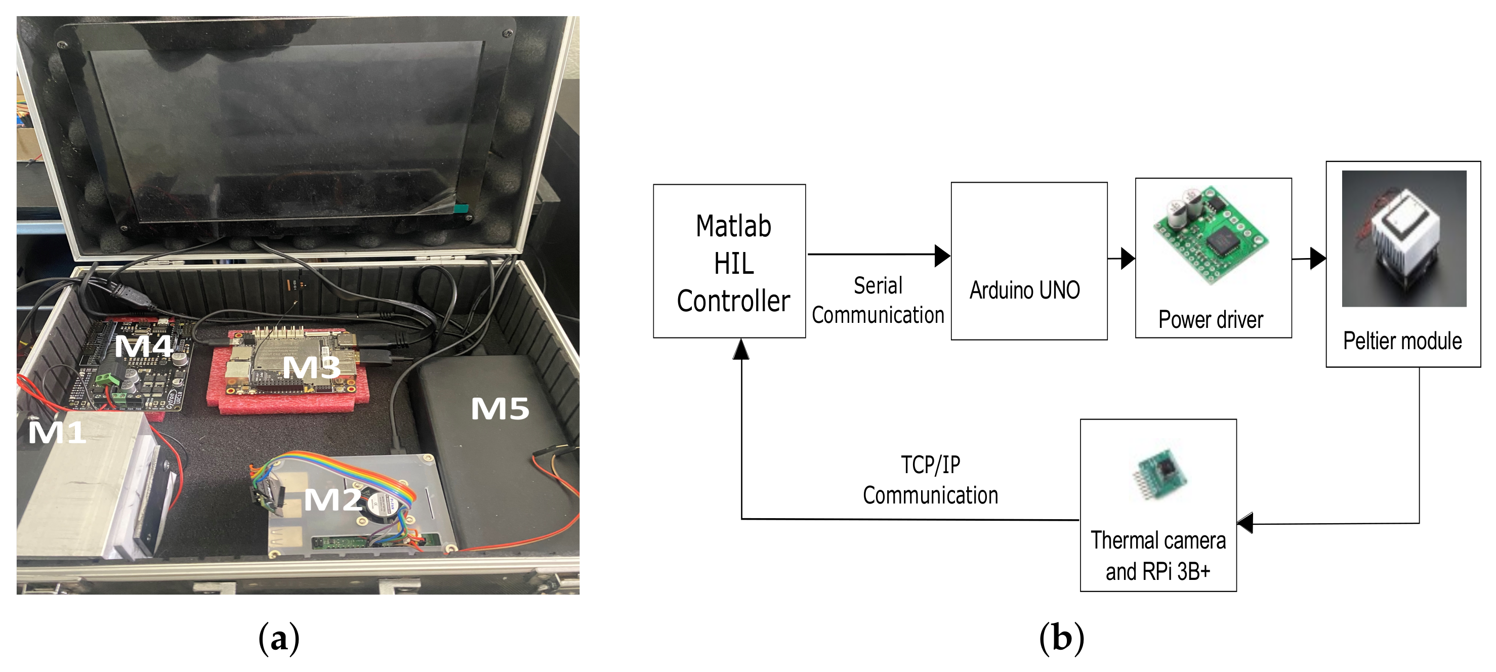
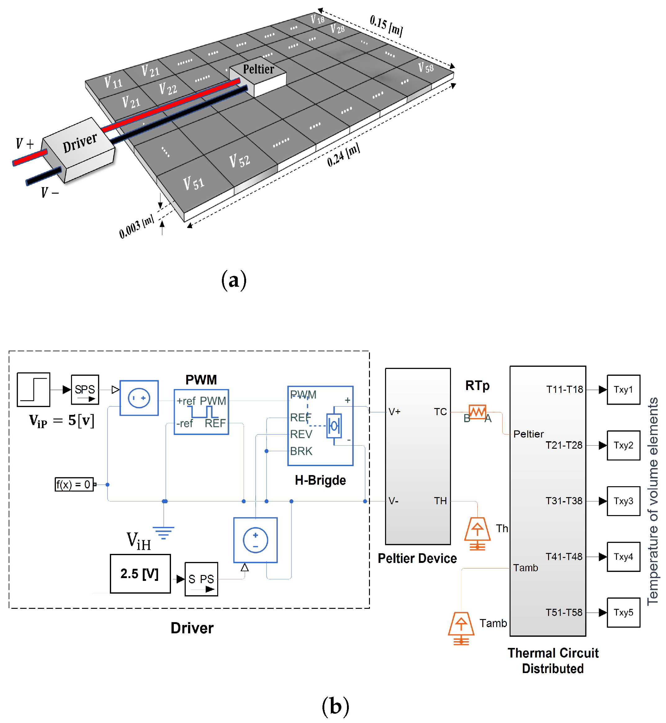
4. A Case Study: Temperature Uniformity Control System

The temperature uniformity control system using real-time thermal infrared (TIR) vision feedback presented in Figure 5 is employed as a case study for VRFT controller design and implementation. The system is composed of a Peltier thermoelectric module (M1) acting as a heating/cooling element, a thermal infrared camera (M2) with TCP/IP communication protocol as a temperature feedback sensor running on a Raspberry Pi and communicated using TCP/IP communication protocol, a LattePanda Embedded board (M3) running Windows 10 that executes Matlab in a hardware in the loop configuration (HIL). The power applied to the Peltier module is controlled using the power driver (M4) via PWM. The platform is equipped with a battery (M5) that provides the power for all of the components in the box with four hours of autonomy. A detailed description of the components of the temperature uniformity control system is presented in Table 1. Likewise, a guide for the system implementation can be found in [30,31].
The main components of the system are the Peltier thermoelectric module and the power driver, whose detailed representations are shown in Figure 6a. They consist of the cascade connection of the driver, the Peltier cell, and an aluminum plate divided in V i j volumetric elements sorted in an 8 × 5 array, where the Peltier and plate are thermally coupled through the volume element V 34 , providing forty measurement points equally separated by 0.03 m.
The system is simulated using Matlab/Simscape, and the corresponding simulation model is shown in Figure 6b containing three main elements: the power driver, the Peltier device, and the plate thermal circuit.
The power driver is configured so that the Peltier cell cools the plate when V i H < 2.5 [V]. For V i H 2.5 [V], the Peltier acts as a heater. The electrical power input to the Peltier cell is regulated by Pulse Width Modulation (PWM), modulating the input voltage in the range 0 [V] V i P 5 [V].
Likewise, the Peltier equivalent circuit is implemented in Simscape using discrete thermal and electrical components as shown in Figure 7. It shows the implemented thermoelectric circuit for the Peltier cell, where the gray blocks represent the Seebeck, Joule, and Peltier effects given by (15)–(17), respectively, where α is the Seebeck coefficient, T c , q c and T h , q h are temperatures and heat on the cold and hot sides of the Peltier, and I , R E are the Peltier current and resistance. The manufacturer’s datasheet specifications for the Peltier coefficients can be found in [32]. Likewise, a complete and detailed description of each parameter of the Peltier and thermal plate modeling can be found in [33]. For this paper, the values employed to simulate the Peltier are α = 0.0421 [V/K], R E = 2.65 [Ω].
F E M = α ( T h T c ) ,
q j = I 2 R E ,
q c = α T c I q h = α T h I .
Finally, the plate heat transfer is modeled by conduction and convection based on the finite element method in a volumetric grid as shown in Figure 8a, where each element is modeled as a thermal resistive–capacitive (RC) network, shown in Figure 8b, with a constant temperature per element volumetric element, as shown in [33]. The Matlab/Simscape implementation of the plate thermal circuit is shown in Figure 8b, where each volume element V n m is represented with a thermal capacitance C T n m and resistance R T n m .

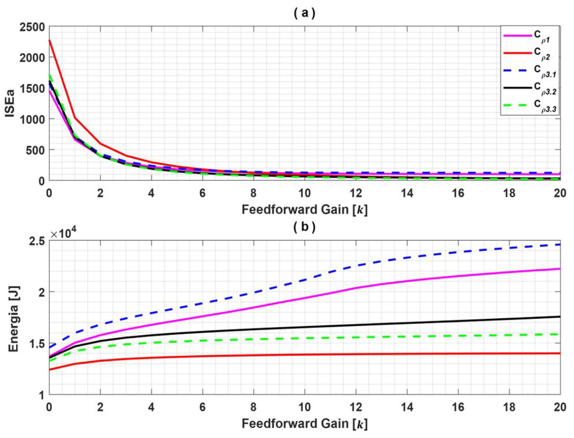
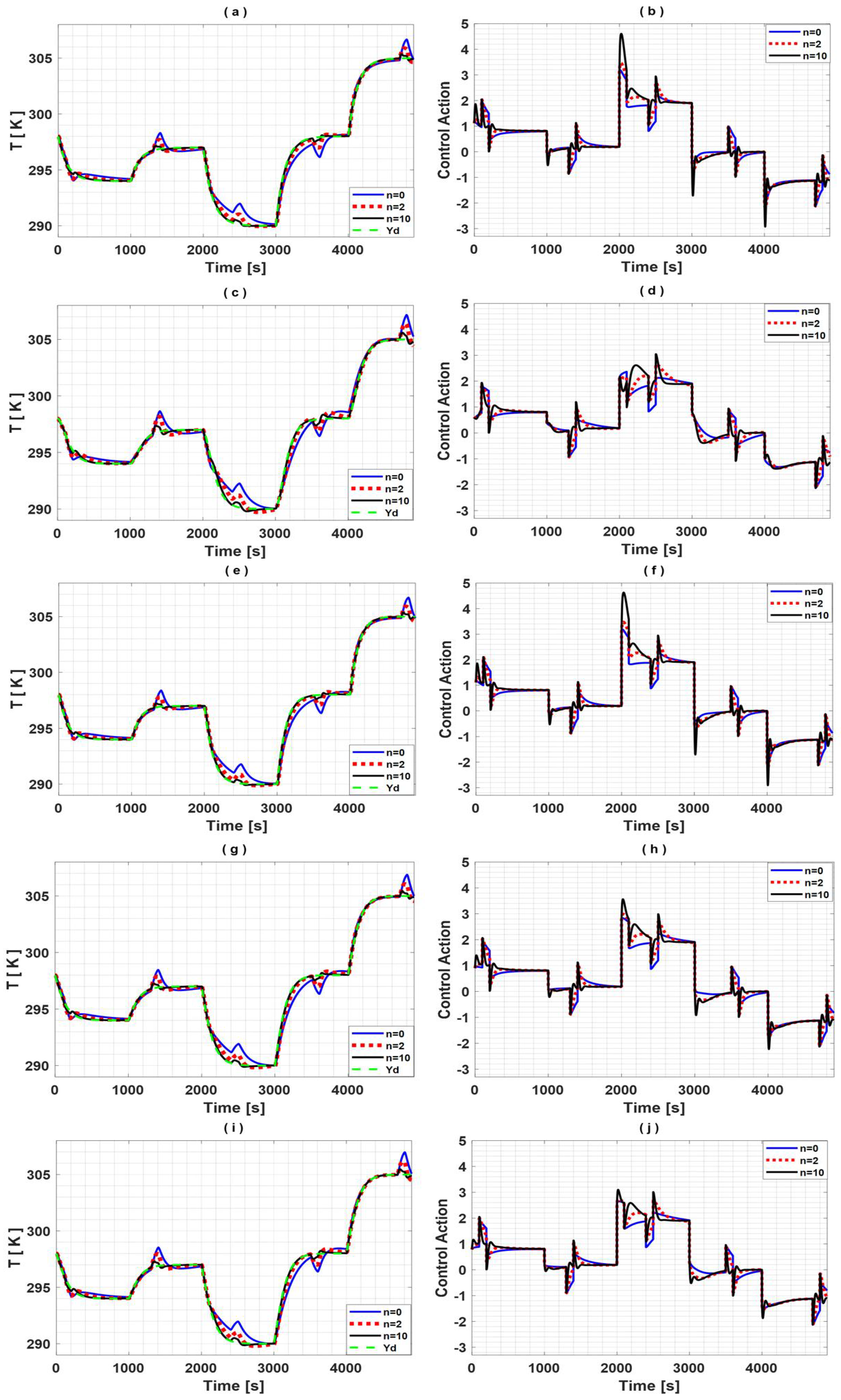
4.1. Feedforward VRFT Controller Design

The VRFT controller synthesis is performed using the procedure shown in Figure 2. Initially, the reference models are defined, which are given by (18):
M 1 ( s ) = w n s + w n , M 2 ( s ) = w n 2 s 2 + 2 w n s + w n 2 , M 3 ( s ) = w n 2 ( T z s + 1 ) s 2 + 2 w n s + w n 2 .
By replacing (18) in (8) and (9), the open-loop transfer functions G 1 , 2 , 3 for the reference models M 1 , 2 , 3 are given by (19):
G 1 ( s ) = w n s , G 2 ( s ) = w n 2 s ( 2 w n + s ) , G 3 ( s ) = w n 2 ( T z s + 1 ) s 2 + w n ( 2 w n T z ) s .
Once the models are defined, the open-loop response of the system is simulated by applying the PRBS signal shown in Figure 9a that sets a ± 100 % duty cycle in random periods to the Peltier system via the power driver to produce the output signal y ( t ) shown in Figure 9b.
So, the virtual error signal e v r is computed by evaluating the response of G 1 , 2 , 3 using y ( t ) as input for w n = 11.66 × 10 3 and T z = [ 1 1.5 w n , 1 2 w n , 1 2.5 w n ] , resulting in five virtual error signals e v r 1 , , 5 , shown in Figure 9c–g. In this case, a first-order compensator is selected as controller C ρ n ’s structure, given by (20), where α , β are the controller coefficients. It is important to notice that for the proposed application, a lag-type compensator is selected ( α 0 < β 0 ) to achieve a smooth response.
C ρ n = α 1 s + α 0 β 1 s + β 0 .
Finally, based on the virtual error signals e v r 1 5 , the VRFT controller can be determined via optimization, which is performed using Matlab’s system identification toolbox, using as the input signal the virtual error e v r 1 , , 5 and the input signal u ( t ) as output following the logic shown in Figure 3. Thus, five controllers are obtained which are defined in (21) with an adjustment of 59.51 % , 64.42 % , 60.48 % , 62.13 % , and 59.95 % , respectively.
C ρ 1 = 278.61 · 10 3 s 1.181 · 10 3 s + 150.48 · 10 6 , C ρ 2 = 136.39 · 10 3 s 1.17 · 10 3 s + 260.29 · 10 6 , C ρ 3.1 = 277.86 · 10 3 s 1.35 · 10 3 s + 175.89 · 10 6 , C ρ 3.2 = 225.23 · 10 3 s 1.281 · 10 3 s + 172.61 · 10 6 , C ρ 3.3 = 196.79 · 10 3 s 1.27 · 10 3 s + 190.58 · 10 6 .
The controllers (21) are evaluated using the simulation model shown in Figure 10, which incorporates the feedforward compensation that uses the reference model and the controller transfer function with a tuning gain k as shown in Figure 4b. The closed-loop responses of the Peltier system and the control actions for the VRFT controllers can be observed in Figure 11. When k = 0 , the feedforward is not active on the system, indicating an error regarding the desired trajectory y d . Likewise, as k increases for k [ 0 ; 2 ; 10 ] , the error is minimized and becomes closer to the reference temperature.
The Integral Square Error I S E for the adaption error e a and the Peltier cumulative energy u indices E p given by (22) and (23) are used as key performance indicators (KPI) for the VRFT controller’s quantitative analysis, where m is the number of samples. Likewise, the performance quantification against the feedforward gain is defined with the indices P D I S E and P I E P , defined in (24)–(25). These indices compute the percentage ratio between the I S E and E P without feedforward I S E ( 0 ) , E P ( 0 ) and those related to the current feedforward employed I S E ( k ) E P ( k ) . The ISE and ITAE performance indices are standard KPIs to evaluate the transient response of the temperature in the Peltier cell given by the proposed VRFT compensators’ C ρ and the PI-IMC and PID-IMC controllers used as benchmark strategies. They also measure the tracking of the system to the desired response given by the reference model. Likewise, E p is a performance index used to quantify the energy consumption of the Peltier Cell. Thus, the proposed indices can be used to provide a metric to determine a reasonable trade-off between the desired model’s reference tracking and the energy consumption to find a suitable tuning rule for the feedforward gain k. Table 2 presents the performance indices for the synthesized VRFT controllers C ρ 1 , , 5 . For example, in the controller C ρ 3.3 , for k = 0 , the adaptation error ISE I S E a ( 0 ) = 6008.65 is bigger for any k. For values of k other than zero, for example, with k = 2 , the adjustment to the desired response is improved by 75%, but the energy consumption increases by 8.7 %.
The effect of the feedforward gain k is further analyzed using the I S E and E P indices as shown in Figure 12. As can be observed, the sweeping of k for 1 k 20 for the controller C ρ 3.3 shows that more energy is required as the adjustment error is minimized. Moreover, for the five controllers C ρ 1 , , 5 , it is noticeable that controller C ρ 1 provides the best fit to the reference model without a feedforward. On the other hand, the controller C ρ 2 presents the greatest deviation compared to the desired response, although it should be noted that it has the lowest energy consumption. Likewise, it is noticeable that the most significant changes in the adjustment to the desired response as k increases occur in the interval 0 < k 6 . However, the performance can be affected for considerably large values of k, which can generate problems with noise and saturation of the control action. Additionally, it can be observed that for k = 4 , the controller C ρ 3.3 achieves the best performance.
On the other hand, the VRTF controller’s robustness is evaluated in the presence of external disturbance in the control action at t = [ 1500 , 2500 , 3500 , 4500 ] s, whose response is shown in Figure 13, and its quantitative evaluation is presented in Table 3. It can be observed that increasing k improves the tracking response and disturbance rejection. However, by increasing k, the control action becomes more aggressive, which, in turn, results in higher energy consumption.
I S E = 1 m j = 0 m e a 2 ( j ) ,
E P = 1 m j = 0 m u 2 ( j ) ,
P D I S E = | I S E ( 0 ) I S E ( k ) I S E ( 0 ) | 100 % ,
P I E P = | E p ( 0 ) E p ( k ) E p ( 0 ) | 100 % .

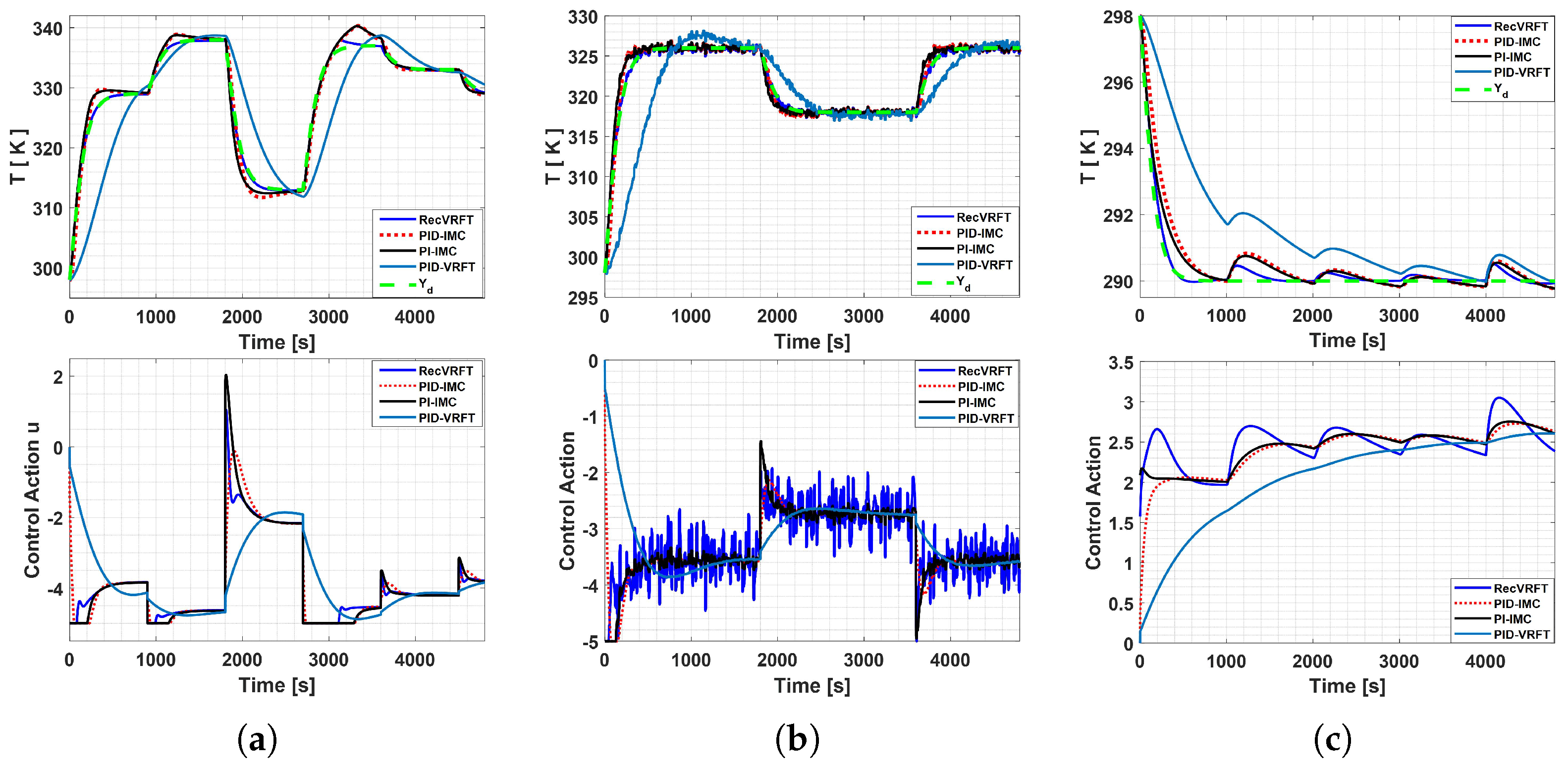
4.2. VRFT against PID Controllers Comparison

The obtained VRFT controllers are compared against three standard PID controllers: one tuned using the VRFT methodology proposed by [34] and PI and PID controllers tuned using the Internal Model Control (IMC) Method. For the PID-VRFT controller tuning, the system input/output response, shown in Figure 9a,b, is used with the reference model (26) and the PID controller structure (27). After the synthesis process, the controller parameters are K p = 18.08 · 10 3 , K d = 2.2 · 10 3 , and K i = 365.03 · 10 6 .
M ( z 1 ) = 2.34 · 10 3 + 67.27 · 10 6 z 1 2.27 · 10 3 z 2 1 1.977 z 1 + 0.9769 z 2 ,
C V R F T P I D = K p + K i s + K d s 1 + T s s .
The design of the PI-IMC and PID-IMC controllers follows the method proposed in [35,36]. As shown in Figure 14a, the controller G c is the inverse of the process model P ˜ 1 followed for a nth-order filter to ensure a proper controller implementation, making λ the only tuning parameter, where G ( s ) is given by (28) and P ˜ is the approximated process model.
G c ( s ) = P ˜ ( λ s + 1 ) n .
So, (28) can be simplified, as shown in Figure 14b, where the resulting controller C I M C can be represented as (29), according to [36].
C I M C ( s ) = G c ( 1 P ˜ G c ) = P ˜ 1 ( λ s + 1 ) n 1 .
Thus, for the PI-IMC controller design, P 1 ˜ is selected as a first-order system calculated using the system response shown in Figure 9, resulting in (30),
P 1 ˜ = a 0 b 1 s + 1 = 5.58 211.51 s + 1 ,
which can be rewritten as (31)
C I M C 1 ( s ) = ( b 1 a 0 λ 1 + 1 a 0 λ 1 s ) .
and, considering the PI controller form in (32), its terms can be compared with (31) to obtain the PI controller’s parameters as K p 1 = b 1 a 0 λ 1 , I 1 = 1 b 1 , resulting in k p 1 = 261.21 e 3 , k i 1 = 4.727 e 3 for λ = 145 .
P I ( s ) = K p 1 ( 1 + I 1 s ) .
For the PID-IMC, a second-order model of the process is obtained, which is given by (33)
P 2 ˜ = c 0 s 2 + d 1 s + 1 + d 0 = 2.929 · 10 3 s 2 + 108.97 · 10 3 s + 545.65 · 10 6 ,
and replacing (33) in (29) with n = 1 , the IMC controller can be expressed as (34)
C I M C 2 ( s ) = s 2 + d 1 s + d 0 ( c 1 s + c 0 ) λ 2 s = ( s 2 + d 1 s + d 0 c 0 λ 2 s ) ( 1 c 1 c 0 + 1 ) .
Thus, comparing the PID controller form given by (35) with (34), the PID controller’s gains can be calculated as K p 2 = d 1 2 c 0 λ 2 , T d 2 = 1 d 1 ; I 2 = d 0 d 1 ; T f 2 = λ 2 2 resulting in K p 2 = 206 e 3 , I 2 = 9.176 , T d 2 = 5 e 3 , and T f 2 = 45 for λ 2 = 45 .
P I D ( s ) = K p 2 ( 1 + I 2 s + T d 2 s ) ( 1 T f 2 s + 1 ) .
The performances of the PI-IMC and PID-IMC controllers are contrasted against the VRFT controller C ρ 3.3 in three operating conditions: nominal, random noise, and external disturbance (adding external thermal load) using the I S E (22), I T A E (36), and E p (23) performance indices. The heat load disturbance used for the testing, shown in Figure 15c, modifies the thermal properties of the V i j volumetric element. The thermal disturbance added to each V i j element is given by C T = m c p , where m is a thermal mass of 1 kg and c p is the specific heat of c p = 3671 J/kg/K. The volumetric elements affected are V i j = [ V 24 , V 25 , V 36 , V 33 ] , and the disturbance is set at each element at the times t = [ 1500 , 2500 , 3500 , 4500 ] s, respectively.
The controller’s response to different temperature setpoints without disturbance (nominal) is shown in Figure 15a and Table 4. It is observed how, with the feedforward, the VRFT control performs better setpoint tracking compared to the PID-VRFT, PI-IMC and PID-IMC controllers. Likewise, the VRFT control action reacts faster to changes in process operation with an energy consumption similar to the other control systems. In the presence of random noise, the controllers response is shown in Figure 15b and Table 5. In this case, the feedforward VRFT is more sensitive to random noise compared with the PI-IMC, and PID-IMC controllers. Finally, when thermal load disturbance at t = [ 1500 , 2000 , 3000 , 4000 ] s is added to the system, the controller’s response is given by Figure 15c and Table 6. It is observed how the feedforward VRFT controller rejects the disturbances more efficiently than the PI-IMC and PID-IMC controllers but requires a greater energy consumption to perform the disturbance rejection.
I T A E = t s m j = 0 m e a 2 ( j ) .

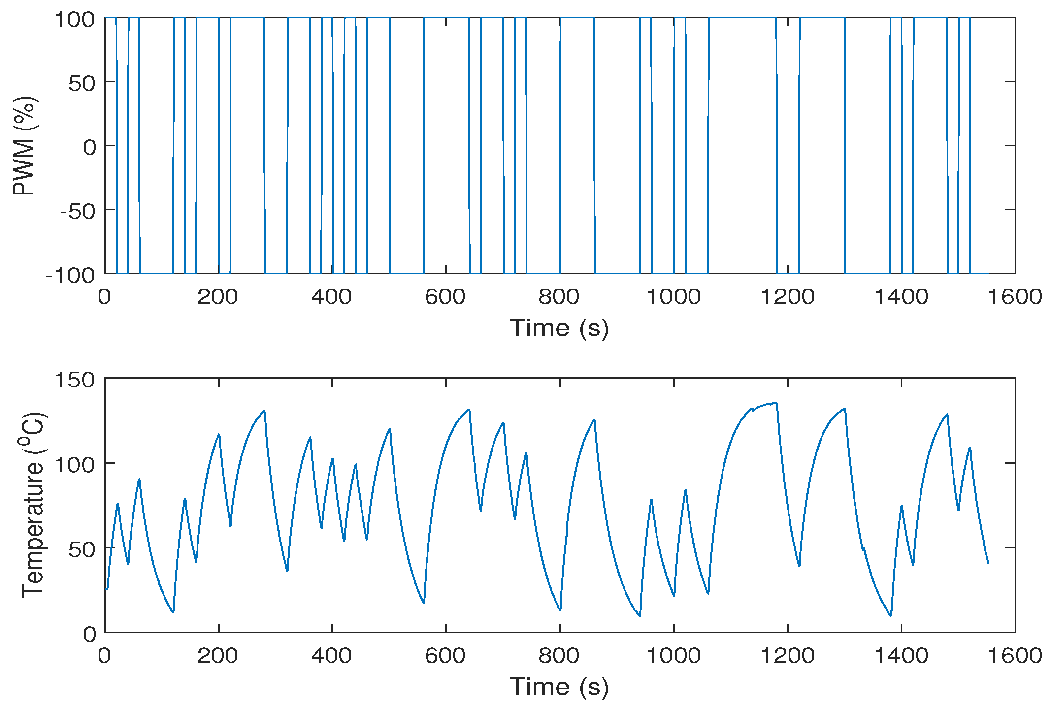
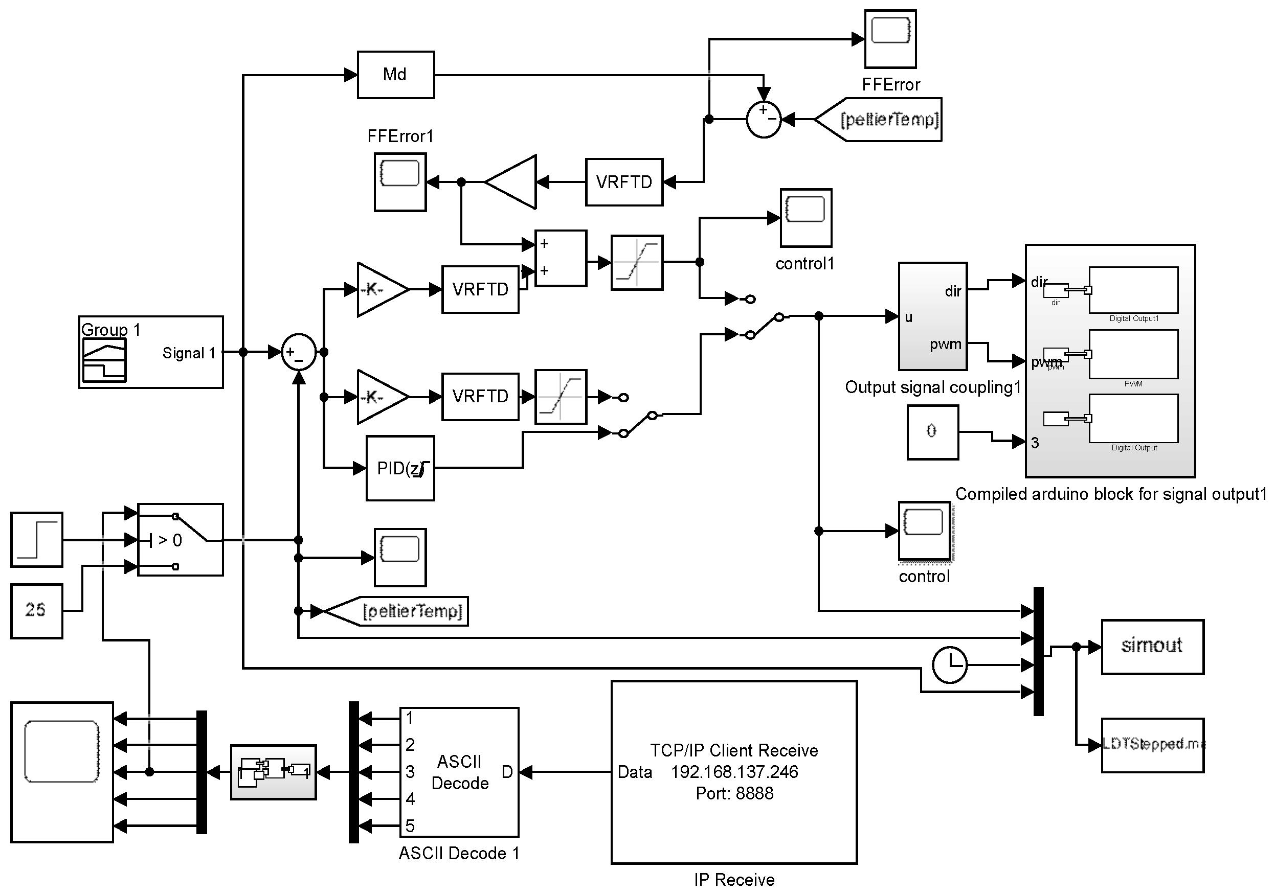
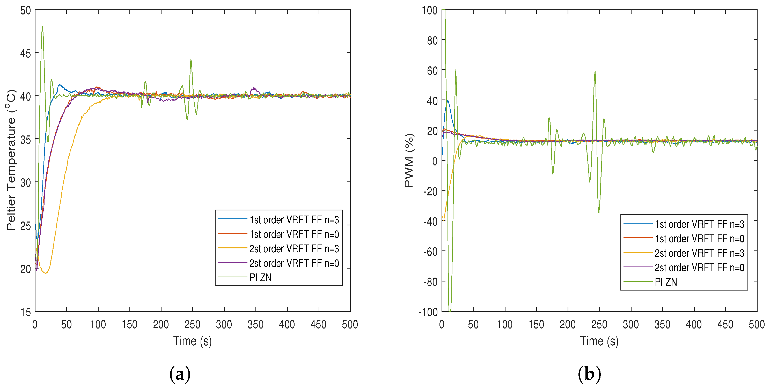
5. Experimental Validation of Recursive VRFT

The experimental platform shown in Figure 5 is employed to perform experimental validation of the proposed recursive VRFT. Thus, the procedure described in Figure 2 is followed again to synthesize the controllers. First, second- and first-order reference models (37) are employed, which are based in G 1 , G 2 defined in (19) with w n = 8 × 10 3 for G 1 and w n = 11.66 × 10 3 for G 2 . Each model includes a low-pass filter H ( s ) = 1 0.1371 s + 1 to compensate for the thermal camera feedback noise. In this case, the low-pass filter deals with the existing temperature randomness. However, it may not be accurate for more complex systems involving more variables with more robust stochastic behavior. Therefore, including a stochasticity awareness mechanism based on the randomness modeling that performs entropy minimization on the VRFT controller synthesis, such as [37,38], could lead to a more robust and stable compensator.
G 1 ( s ) = w n 2 s ( 2 w n + s ) H ( s ) G 2 ( s ) = w n s H ( s ) .
Then, the open-loop response of the system is obtained by applying a PRBS signal, which is shown in Figure 16. So, the virtual error signals are computed using (37) along with the data in Figure 16. Thus, the VRFT controllers are synthesized using the compensator structures (38) and (39), along with the reference models (37), to obtain the first- and second-order controllers, respectively.
C 1 ( s ) = A 1 s + A 0 B 1 s + B 0 = 2.75 s + 0.1 s + 640 · 10 6 ,
C 2 ( s ) = A 2 s 2 + A 1 s + A 0 B 2 s 2 + B 1 s + B 0 = 2.12 s 2 + 0.11 s + 543 · 10 6 s 2 + 6.6 · 10 3 s + 6.38 · 10 12 .
Likewise, a PI controller is tuned using the Ziegler–Nichols method to compare the performance of the obtained VRFT controllers whose gains are k p = 25.05 k i = 0.713 . The controller implementation is performed using a hardware in the loop configuration, shown in Figure 17, that can be downloaded from https://github.com/tartanus/Recursive-VRFT (accessed on 16 October 2023). As can be observed, the VRFT controllers are implemented in Simulink with real-time TCP/IP feedback for the infrared camera. Likewise, the PWM is applied using an Arduino board communicated via serial communication.
The response and control action for the VRFT controllers with a feedforward gain ( k = 3 ), without a feedforward ( k = 0 ), and the PI controller are shown in Figure 18a,b. As can be observed, the first-order VRFT controller with a feedforward has a better response, reaching a settling time of 100 s with a reasonable overshoot. Moreover, the second-order VRFT controller performance induces a slower response without feedforward compensation. Likewise, the PI controller has a faster settling time but a high overshoot and sensitivity in the presence of small feedback fluctuations. In this case, the presence of jitter during the time range [150–300] s is caused by the infrared thermal camera. It performs an automatic recalibration at 169 s to adjust the brightness and irradiance, which can be considered an external disturbance to the system. Thus, the high proportional and integral gains obtained for the ZN-PI controller compared with the gains on the C1 and C2 controllers synthesized using the recursive VRFT method make the system more sensitive to external disturbances and the presence of random noise, causing the aggressive response on the ZN-PI controller. In terms of control action, the first-order VRFT requires slightly more energy in the beginning compared with the second-order controller but provides a fast correction of the setpoint. Therefore, we can say that for the Peltier system, the VRFT controller with a feedforward can improve the system response as well as improve its robustness in the presence of small disturbances.

6. Conclusions and Future Works

This paper presented a framework for synthesizing VRFT controllers with a feedforward using an optimization approach that allows the parameter calculation for different controller architectures based on a desired reference model and the system’s open-loop response. It incorporates a feedforward strategy that minimizes the adjustment error between the desired reference model and system output. It employs a proportional gain k times the synthesized controller, providing an additional corrective control action that minimizes the adjustment error. The method was tested for the VRFT controller design of a temperature uniformity control system, using first and second-order reference models. The simulation and experimental results indicate that the VRFT controller with a feedforward improves the system’s setpoint tracking response and external disturbance rejection, which increases as the feedforward gain k is increased. Due to the system’s nature, the first-order compensator responds better than the high-order synthesized controllers. However, it is important to note that for more complex systems and controller architectures, the proposed VRFT synthesis can provide a reasonable and robust controller response based only on the available open-loop system’s data. In future work, the proposed VRFT controller synthesis method can be modified for online controller tuning based on the open-loop or closed-loop system responses while ensuring its robustness and stability. Likewise, the evaluation of different reference models and controller architectures, such as non-linear or multivariable controls, is proposed.

Author Contributions

Conceptualization, J.G.A., L.A., J.V. and Y.C.; methodology, J.G.A. and L.A.; software, J.G.A. and L.A.; validation, J.G.A., L.A. and J.V.; formal analysis, L.A. and Y.C.; investigation, J.G.A. and L.A.; resources, J.G.A., L.A., J.V. and Y.C.; data curation, J.G.A., L.A. and J.V.; writing—original draft preparation, J.G.A., L.A. and J.V.; writing—review and editing, J.G.A., L.A., J.V. and Y.C.; visualization, J.G.A. and L.A.; supervision, L.A. and Y.C.; project administration, L.A.; funding acquisition, L.A. All authors have read and agreed to the published version of the manuscript.

Funding

This research received no external funding.

Institutional Review Board Statement

Not applicable.

Informed Consent Statement

Not applicable.

Data Availability Statement

Not applicable.

Conflicts of Interest

The authors declare no conflict of interest.

References

  1. Hou, Z.S.; Wang, Z. From model-based control to data-driven control: Survey, classification and perspective. Inf. Sci. 2013, 235, 3–35. [Google Scholar] [CrossRef]
  2. Guardabassi, G.O.; Savaresi, S.M. Virtual reference direct design method: An off-line approach to data-based control system design. IEEE Trans. Autom. Control 2000, 45, 954–959. [Google Scholar] [CrossRef]
  3. David, J.; Fernández, R. Extensions and Applications of the Virtual Reference Feedback Tuning. Ph.D. Thesis, Universitat Autònoma de Barcelona, Barcelona, Spain, 2011. [Google Scholar]
  4. Beninca, M.R. Virtual Reference Feedback Tuning of Controllers Parametrized Using Orthonormal Basis Functions. Ph.D. Thesis, Paraná Federal Univeristy, Parana, Brazil, 2015. [Google Scholar]
  5. Imchen, S.; Das, D.K. Scheduling of distributed generators in an isolated microgrid using opposition based Kho-Kho optimization technique. Expert Syst. Appl. 2023, 229, 120452. [Google Scholar] [CrossRef]
  6. Tian, J.; Zeng, Y.; Ji, L.; Zhu, H.; Guo, Z. Control Method of Cold and Hot Shock Test of Sensors in Medium. Sensors 2023, 23, 6536. [Google Scholar] [CrossRef] [PubMed]
  7. Wang, S.; Zhao, B.; Yi, S.; Zhou, Z.; Zhao, X. GAPSO-Optimized Fuzzy PID Controller for Electric-Driven Seeding. Sensors 2022, 22, 6678. [Google Scholar] [CrossRef] [PubMed]
  8. Pradhan, S.K.; Subudhi, B. Position control of a flexible manipulator using a new nonlinear self-tuning PID controller. IEEE/CAA J. Autom. Sin. 2020, 7, 136–149. [Google Scholar] [CrossRef]
  9. Zhu, G.; Ma, Y.; Hu, S. Event-Triggered Adaptive PID Fault-Tolerant Control of Underactuated ASVs Under Saturation Constraint. IEEE Trans. Syst. Man Cybern. Syst. 2023, 53, 4922–4933. [Google Scholar] [CrossRef]
  10. Chen, Q.; Wang, Y.; Song, Y. Tracking Control of Self-Restructuring Systems: A Low-Complexity Neuroadaptive PID Approach With Guaranteed Performance. IEEE Trans. Cybern. 2023, 53, 3176–3189. [Google Scholar] [CrossRef]
  11. Sánchez-Palma, J.; Ordoñez-Ávila, J.L. A PID Control Algorithm with Adaptive Tuning Using Continuous Artificial Hydrocarbon Networks for a Two-Tank System. IEEE Access 2022, 10, 114694–114710. [Google Scholar] [CrossRef]
  12. Shiro, M.; Matsui, Y. Data-Driven Control and Learning Systems. IEEE Trans. Ind. Electron. 2017, 64, 4070–4075. [Google Scholar] [CrossRef]
  13. Hjalmarsson, H.; Gevers, M.; Gunnarsson, S.; Lequin, O. Iterative feedback tuning: Theory and applications. IEEE Control Syst. Mag. 1998, 18, 26–41. [Google Scholar] [CrossRef]
  14. Kutz, J.N.; Brunton, S.L.; Brunton, B.W.; Proctor, J.L. Dynamic Mode Decomposition; Society for Industrial and Applied Mathematics: Philadelphia, PA, USA, 2016. [Google Scholar] [CrossRef]
  15. Chen, Y.; Wen, C. Iterative Learning Control: Convergence, Robustness and Applications, 1st ed.; Springer: London, UK, 1999; p. 204. [Google Scholar] [CrossRef]
  16. Ariyur, K.; Krstic, M. Real-Time Optimization by Extremum-Seeking Control; Wiley-Interscience: Hoboken, NJ, USA, 2003. [Google Scholar]
  17. Hou, Z.; Jin, S. Model Free Adaptive Control: Theory and Applications; CRC Press: Boca Raton, FL, USA, 2013. [Google Scholar]
  18. Safonov, M.; Tsao, T.C. The unfalsified control concept and learning. IEEE Trans. Autom. Control 1997, 42, 843–847. [Google Scholar] [CrossRef]
  19. Spall, J.C. Introduction to Stochastic Search and Optimization, 1st ed.; John Wiley & Sons, Inc.: Hoboken, NJ, USA, 2003. [Google Scholar]
  20. Lecchini, A.; Campi, M.C.; Savaresi, S.M. Sensitivity shaping via virtual reference feedback tuning. In Proceedings of the Proceedings of the 40th IEEE Conference on Decision and Control (Cat. No.01CH37228), Orlando, FL, USA, 4–7 December 2001; Volume 1, pp. 750–755. [Google Scholar] [CrossRef]
  21. Campi, M.C.; Lecchini, A.; Savaresi, S.M. Virtual reference feedback tuning: A direct method for the design of feedback controllers. Automatica 2002, 38, 1337–1346. [Google Scholar] [CrossRef]
  22. Sato, T.; Sakai, Y.; Kawaguchi, N.; Arrieta, O. Dual-Rate Data-Driven Virtual Reference Feedback Tuning: Improvement in Fast-Tracking Performance and Ripple-Free Design. IEEE Access 2021, 9, 144426–144437. [Google Scholar] [CrossRef]
  23. Remes, C.L.; Gomes, R.B.; Flores, J.V.; Líbano, F.B.; Campestrini, L. Virtual Reference Feedback Tuning Applied to DC–DC Converters. IEEE Trans. Ind. Electron. 2021, 68, 544–552. [Google Scholar] [CrossRef]
  24. Ding, Y.; Xu, N.; Ren, L.; Hao, K. Data-Driven Neuroendocrine Ultrashort Feedback-Based Cooperative Control System. IEEE Trans. Control. Syst. Technol. 2015, 23, 1205–1212. [Google Scholar] [CrossRef]
  25. Campestrini, L.; Eckhard, D.; Chía, L.A.; Boeira, E. Unbiased MIMO VRFT with application to process control. J. Process Control 2016, 39, 35–49. [Google Scholar] [CrossRef]
  26. Chiluka, S.K.; Ambati, S.R.; Sonawane, S.H.; Seepana, M.M.; Babu Gara, U.B. Robust IMC-PID Controller Design using VRFT: Theoretical and Experimental Investigation; IFAC-PapersOnLine. In Proceedings of the 7th International Conference on Advances in Control and Optimization of Dynamical Systems ACODS 2022, Silchar, India, 22–25 February 2022; Volume 55, pp. 241–246. [Google Scholar] [CrossRef]
  27. Vilanova, R.; Visioli, A. PID Control in the Third Millennium: Lessons Learned and New Approaches; Springer: London, UK, 2012. [Google Scholar]
  28. Formentin, S.; Campi, M.C.; Carè, A.; Savaresi, S.M. Deterministic Continuous-Time Virtual Reference Feedback Tuning (VRFT) with Application to PID Design. Syst. Control Lett. 2019, 127, 25–34. [Google Scholar] [CrossRef]
  29. Freddy, F.; Valderrama Gutierrez, F.O.R. Novel Data-Driven Control Approaches. Ph.D. Thesis, Pontifical Javerian University, Bogota, Colombia, 2019. [Google Scholar]
  30. Viola, J.; Radici, A.; Dehghan, S.; Chen, Y. Low-cost real-time vision platform for spatial temperature control research education developments. In Proceedings of the International Design Engineering Technical Conferences and Computers and Information in Engineering Conference, Anaheim, CA, USA, 18–21 August 2019; American Society of Mechanical Engineers: New York, NY, USA, 2019; Volume 59292, p. V009T12A030. [Google Scholar]
  31. Viola, J.; Oziablo, P.; Chen, Y. A Portable and Affordable Networked Temperature Distribution Control Platform for Education and Research. IFAC-PapersOnLine 2020, 53, 17530–17535. [Google Scholar] [CrossRef]
  32. Lineykin, S.; Ben-Yaakov, S. Modeling and analysis of thermoelectric modules. IEEE Trans. Ind. Appl. 2007, 43, 505–512. [Google Scholar] [CrossRef]
  33. Araque–Mora, J.; Angel, L. Distributed Equivalent Circuit for Modeling Heat Transfer Process in a Thermoelectric System. In Proceedings of the 2021 IEEE 5th Colombian Conference on Automatic Control (CCAC), Ibague, Colombia, 19–22 October 2021; pp. 326–331. [Google Scholar] [CrossRef]
  34. Carè, A.; Torricelli, F.; Campi, M.C.; Savaresi, S.M. A Toolbox for Virtual Reference Feedback Tuning (VRFT). In Proceedings of the 2019 18th European Control Conference (ECC), Naples, Italy, 25–28 June 2019; pp. 4252–4257. [Google Scholar] [CrossRef]
  35. Angel, L.; Viola, J.; Paez, M. Speed control of a motor-generator system using internal model control techniques. In Proceedings of the 2017 IEEE 3rd Colombian Conference on Automatic Control (CCAC), Cartagena, Colombia, 18–20 October 2017; pp. 1–6. [Google Scholar] [CrossRef]
  36. Nath, U.M.; Dey, C.; Mudi, R.K. Review on IMC-based PID Controller Design Approach with Experimental Validations. IETE J. Res. 2021, 69, 1640–1660. [Google Scholar] [CrossRef]
  37. Mifeng Ren, Q.Z.; Zhang, J. An introductory survey of probability density function control. Syst. Sci. Control. Eng. 2019, 7, 158–170. [Google Scholar] [CrossRef]
  38. Zhang, Q.; Zhou, Y. Recent Advances in Non-Gaussian Stochastic Systems Control Theory and Its Applications. Int. J. Netw. Dyn. Intell. 2022, 1, 111–119. [Google Scholar] [CrossRef]
Figure 1. Classic VRFT framework [28].
Machines 11 00975 g001
Figure 2. Recursive VRFT controller synthesis framework for a general controller architecture design based on an optimization algorithm to find controller parameters according to (4).
Machines 11 00975 g002
Figure 3. Recursive VRFT signal architecture. (a) shows the the virtual error E v ( s ) calculation using the closed-loop model M ( s ) , which feeds the identification algorithm to find the controller parameters. Likewise, (b) simplifies the computation of E v ( s ) by using the open-loop G ( s ) reference model.
Machines 11 00975 g003
Figure 4. VRFT feedforward controller proposal. (a) Model reference scheme of VRFT; (b) feedback feedforward VRFT control system.
Machines 11 00975 g004
Figure 5. Case study: real-time vision feedback infrared temperature uniformity control system. (a) Physical asset; (b) HIL closed-loop controller implementation using Simulink/Arduino.
Machines 11 00975 g005
Figure 6. Temperature uniformity system process. (a) The 3D schematic including driver, Peltier module, and the volumetric modeled thermal plate; (b) Simulink/Simscape process model representation.
Machines 11 00975 g006
Figure 7. Peltier RC thermal circuit equivalent assembly in Simulink/Simscape including Peltier, Seebeck, and Joule effects.
Machines 11 00975 g007
Figure 8. Thermal plate interaction modeling: (a) based on RC network for individual volumetric elements and (b) Simulink/Simscape model.
Machines 11 00975 g008
Figure 9. Peltier open-loop system identification. (a) Input ( P R B S signal with 1 / 10 Hz periods), (b) Peltier temperature output T ( t ) , and (cg) virtual errors for the reference models G 1 5 ( s ) .
Machines 11 00975 g009
Figure 10. Feedforward VRFT controller implemented in Simulink composed by the reference models M 1 , , 5 , the feedforward error compensation C a , and the temperature uniformity control system.
Machines 11 00975 g010
Figure 11. Temperature performance of controllers C ρ 1 , , 5 (ae) and their control actions (fj) for different feedforward gains k. The feedforward compensates the tracking error but induces control action saturation as k increases.
Machines 11 00975 g011
Figure 12. Sweeping of the adjustment error gain k vs. I S E and E p for the synthesized controllers C ρ . (a) explains the variation of I S E against k showing a error reduction for higher values of k. Likewise, (b) describes the variation of E p against k showing an evident increment of energy consumption for higher k. Therefore, an acceptable performance is reached for 6 k 8 with a good trade-off between error minimization and energy consumption.
Machines 11 00975 g012
Figure 13. Temperature performance of controllers C ρ 1 , , 5 (ae) and their control actions (fj) for different feedforward gains k in the presence of external disturbance in the control action at t = [ 1500 , 2500 , 3500 , 4500 ] s. The feedforward provides a disturbance rejection but increases the rejection energy required as k is bigger.
Machines 11 00975 g013
Figure 14. IMC controller framework design. (a) G c is the inverse of the estimated process P ˜ 1 plus a low-pass filter to obtain a proper and realizable controller. (b) shows the rearrangement of the IMC controller as a PI feedback regulator C I M C given by (32).
Machines 11 00975 g014
Figure 15. Recursive feedforward VRFT and PI/PID controllers’ response: (a) temperature setpoint tracking; (b) random noise in the feedback loop; and (c) external disturbance produced by thermal load on the plate. The VRFT controller with a feedforward provides a more robust response for tracking and external disturbance.
Machines 11 00975 g015
Figure 16. Temperature uniformity system open-loop response for a PRBS input signal.
Machines 11 00975 g016
Figure 17. Matlab/Simulink feedforward VRFT HIL implementation. The implementation includes the TCP-IP feedback from thermal camera, VRFT controller, and feedback scheme with output interface using Arduino.
Machines 11 00975 g017
Figure 18. Temperature uniformity control response (a) for the VRFT and PI controllers computed control action (b) for a 40 °C setpoint. As can be observed, the time response (a) for the first-order VRFT controller with Feedforward gain k = 3 provides a faster response with less sensitivity to random noise compared with the other controllers. Also, the control action (b) of the VRFT first and second controller controllers provides an smooth and robust response compared with the PI-ZN in the presence of external disturbances as at t = 250 s caused by the thermal camera automatic recalibration.
Machines 11 00975 g018
Table 1. Temperature Uniformity Control System Specifications.
ComponentFeatures
FLIR lepton thread
Infrared thermal camera
Wavelength: 8 to 14 μm
Resolution: 80 × 60 pixels
Accuracy: ±0.5 °C
TEC1-12706
Peltier Module
Q m a x = 50  W
Δ T m a x = 75 C
I M a x = 6.4  A
V m a x = 16.4  V
MC33926 DC
Power Driver
Input: 0–5 V
Output: 0–12 V
Peak Current: 5 A
LattePanda board5 inch Windows 10 64 bits PC
Intel Atom μ p
4 GB of RAM
Built-in Arduino Leonardo board
Table 2. VRFT controllers quantitative performance for different feedforward gain k on setpoint tracking tasks.
ControllerGain
k
ISEa P D I S E a [%] E P [J] P I E p [%]
C ρ 1 05227.240.046,981.760.0
21997.8161.854,220.9115.4
51391.2173.461,055.7530.0
101328.2074.670,605.2550.3
C ρ 2 012,341.970.041,406.340.0
22745.8577.843,332.894.7
51028.7991.745,161.899.1
10406.0896.746,495.3012.3
C ρ 3.1 05440.110.049,806.090.0
22250.3858.658,327.4817.1
51733.0868.168,945.0638.4
101724.1268.378,772.2858.2
C ρ 3.2 05225.760.045,982.250.0
21466.7471.950,930.1010.8
5666.4587.254,343.6518.2
10409.3392.259,674.2029.8
C ρ 3.3 06008.650.044,689.470.0
21503.1075.048,560.128.7
5578.6990.450,752.7413.6
10264.0695.652,740.1318.0
Table 3. VRFT controllers quantitative performance for different feedforward gain k on setpoint tracking tasks in the presence of thermal load disturbance.
ControllerGain
k
ISEa P D I S E a [%] E P [J] P I E p [%]
C ρ 1 01982.440.010,466.430.0
2496.8774.911,650.0611.3
5176.8691.112,217.2716.7
1068.7396.512,947.2723.7
C ρ 2 02534.2109702.820.0
2918.8263.710,496.298.2
5420.3783.410,647.119.7
10179.4792.910,708.0710.4
C ρ 3.1 01849.710.010,893.320.0
2467.9574.712,094.3511.0
5169.1590.912,697.6716.6
1066.7896.413,523.1624.1
C ρ 3.2 02069.790.010,468.950.0
2562.1372.811,443.269.3
5208.8789.911,744.0412.2
1077.5996.311,944.2814.1
C ρ 3.3 02153.580.010,299.650.0
2625.0771.011,186.998.6
5243.0088.711,399.5510.7
1091.9995.711,485.1011.5
Table 4. Process performance by changing the operating point.
Control
System
ISE a ITAE a E P
R e c u r s i v e - V R F T 1009.653,543,789.93120,879.63
I M C - P I D 8796.4010,322,383.31122,416.94
I M C - P I 10,426.4410,251,645.23124,000.37
V R F T - P I D 187,220.9335,687,688.87113,657.34
Table 5. Control system performance with feedback noise.
Control
System
ISE a ITAE a E P
R e c u r s i v e - V R F T 718.743,275,236.0883,427.47
I M C - P I D 2644.184,284,296.6583,738.90
I M C - P I 4079.304,801,885.6084,462.43
V R F T - P I D 91,064.2114,019,821.7577,352.45
Table 6. Process performance applying thermal load on the metallic plate.
Control
System
ISE a ITAE a E P
R e c u r s i v e - V R F T 193.761,228,571.9149,499.74
I M C - P I D 1619.682,599,650.8446,954.49
I M C - P I 736.252,306,393.5347,797.99
V R F T - P I D 16,352.037,674,062.4736,716.94
Disclaimer/Publisher’s Note: The statements, opinions and data contained in all publications are solely those of the individual author(s) and contributor(s) and not of MDPI and/or the editor(s). MDPI and/or the editor(s) disclaim responsibility for any injury to people or property resulting from any ideas, methods, instructions or products referred to in the content.

