A Sliding Mode Approach-Based Adaptive Steering Control Algorithm for Path Tracking of Autonomous Mobility with Weighted Injection

Abstract

The increasing complexity of mathematical models developed as part of the recent advancements in autonomous mobility platforms has led to an escalation in uncertainty. Despite the intricate nature of such models, the detection, decision, and control methods for autonomous mobility path tracking remain critical. This study aims to achieve path tracking based on pixel-based control errors without parameters in the mathematical model. The proposed approach entails deriving control errors from a multi-particle filter based on a camera, estimating the error dynamics coefficients through a recursive least squares (RLS) approach, and using the sliding mode approach and weighted injection to formulate a cost function that leverages the estimated coefficients and control errors. The resultant adaptive steering control expedites the convergence of control errors towards zero by determining the magnitude of the injection variable based on the control errors and the finite-time convergence condition. The efficacy of the proposed approach is evaluated through an S-curved and elliptical path using autonomous mobility equipped with a single steering and driving module. The results demonstrate the capability of the approach to reasonably track target paths through driving and steering control facilitated by a multi-particle filter and a lidar-based obstacle detection system.

1. Introduction

Autonomous mobility is undergoing development across various platforms, catering to specific use cases that enhance user convenience and operational efficiency. These platforms encompass domains such as smart factories, smart farms, automobiles, and healthcare facilities. Within the realm of autonomous mobility, sensors, including cameras, lidars, and radars, play a pivotal role in obstacle detection, path tracking, and environmental perception. Additionally, the strategic placement of these sensors is a crucial consideration for effective autonomous operation. However, the diversification of autonomous mobility platforms introduces heightened complexity and uncertainty in mathematical modeling. The implications of such uncertainty can exert detrimental effects on control mechanisms. Hence, the development of perception, decision, and control techniques that account for disturbances and uncertainties is of paramount significance.

Zhang et al., employed camera-derived lane detection and lateral error calculations to propose a path-tracking algorithm for intelligent electric vehicles. This algorithm integrated a linear quadratic regulator based on error dynamics and sliding mode control [1]. Muthalagu et al., presented an algorithm that utilizes vision or camera data to detect straight lines, curves, and steep lanes through a combination of edge detection, polynomial regression, perspective transformation, and histogram analysis [2]. Jiao et al., introduced a lane detection approach that incorporated a multi-lane following Kalman filter. Their algorithm centered on lane voting vanishing points derived from camera-based original images for simplified grid-based noise filtering [3]. Miyamoto et al., devised a unique road-following technique that combines image processing with semantic segmentation. The practicality of this method was confirmed through a 500 m test drive employing three webcams and a robot [4]. De Morais et al., outlined a hybrid control architecture merging deep reinforcement learning with a robust linear quadratic regulator. This architecture leveraged RGB information from vision-based images to maintain an autonomous vehicle within the lane center, even amidst uncertainties and disturbances [5]. Khan et al., proposed an efficient conventional neural network approach featuring minimal parameters and a lightweight structural model, which can be implemented in embedded devices for accurate lane detection using vision or camera-based images [6].

Recent research dedicated to the advancement of human-following mobile robots has focused on object tracking algorithms leveraging techniques such as histogram of oriented gradient, support vector machines, color histogram comparison [7], and correlation filters utilizing RGB and pixel data [8]. Investigations are also in progress to devise path tracking for mobile robots that incorporate the robustness of sliding mode control [9,10] with the uncertainties and disturbances inherent in mathematical models and parameters and reflect the physical characteristics of the robot based on a model predictive controller [11,12]. Additionally, some studies are exploring path-following strategies for mobile robots, harnessing GPS and vision or camera sensors [13,14].

The particle filter, which is suitable for nonlinear and non-Gaussian filtering, finds application across diverse signal processing fields and mathematical models. It is widely utilized for visual tracking and localization using vision or cameras. Camera-based visual tracking is used in multiple applications ranging from automated surveillance to object tracking and medical care. Since the surrounding environment continuously changes when an object moves, studies are being conducted on object tracking that is robust despite changes in lighting, background confusion, and scale [15,16,17,18]. In the context of autonomous driving and vehicle navigation, researchers are actively engaged in refining location estimation through particle filter-based approaches for autonomous vehicles and robots. This aims to secure accurate location determination within indoor environments, mitigating the uncertainties associated with GPS sensors [19,20,21]. A controller based on a mathematical model for path following autonomous vehicles and robots may adversely affect control performance due to uncertainties in parameters and mathematical models, as well as disturbances in various driving situations. Studies are currently being conducted to enhance the performance of path-tracking control by compensating for uncertainties and disturbances in parameters and mathematical models. This is achieved using neural networks and deep reinforcement [22,23,24,25,26], as well as adaptive rules [27,28].

Previous research has explored methodologies for lane and object detection utilizing pixel and RGB data from camera images, particle filters, and image processing techniques. Furthermore, ongoing investigations have validated the evolution of robust path-tracking control algorithms based on artificial intelligence and adaptive principles. These algorithms are designed to counterbalance uncertainties and disturbances inherent in mathematical models and parameters. This framework has culminated in diverse forms of autonomous mobility tailored to distinct use cases, such as human following and path tracking, to enhance worker safety and operational efficiency. However, these path tracking algorithms based on artificial intelligence require extensive learning methods using reliable and sufficient training data that represent normal path tracking conditions. Additionally, since the results are derived from learned data, there is a limitation in the determination and quantification of path misjudgment, especially when obstacles are present in the path. Therefore, the present study proposes an adaptive steering control algorithm for autonomous mobility systems. The central objective is to enhance worker convenience and operational efficiency by tracking color-coded paths in initial infrastructure settings, such as smart farms and factories, with adaptive control algorithms without depending on the parameters of complex mathematical models. Additionally, by utilizing a particle filter to detect the target path, it becomes feasible to develop a functional safety algorithm that can identify in real-time path misjudgment with distance index. The control errors used for the autonomous path-tracking mechanism were derived through a multi-particle filter-based approach based on camera RGB data. The adaptive steering control algorithm harnesses the control error alongside the estimated coefficients derived from simplified error dynamics via an RLS methodology. The cost function incorporates the sliding mode approach and weighted injection while considering the control error. The weighted injection ensures swift convergence of control errors to zero, as it dynamically adjusts the injection magnitude based on the control error magnitude while also considering the finite-time convergence condition. To evaluate the performance of the adaptive steering control algorithm, tests were conducted on S-curved and elliptical paths using autonomous mobility with a single steering and driving module.

The remainder of this paper is structured as follows. Section 2 introduces the concept of control error derivation through a multi-particle filter mechanism and describes the adaptive steering control algorithm. Section 3 discusses the performance of the proposed algorithm in tests conducted in working environments using developed autonomous mobility. Finally, Section 4 and Section 5 present the conclusions and future avenues of research.

2. Adaptive Path Tracking Algorithm of Autonomous Mobility

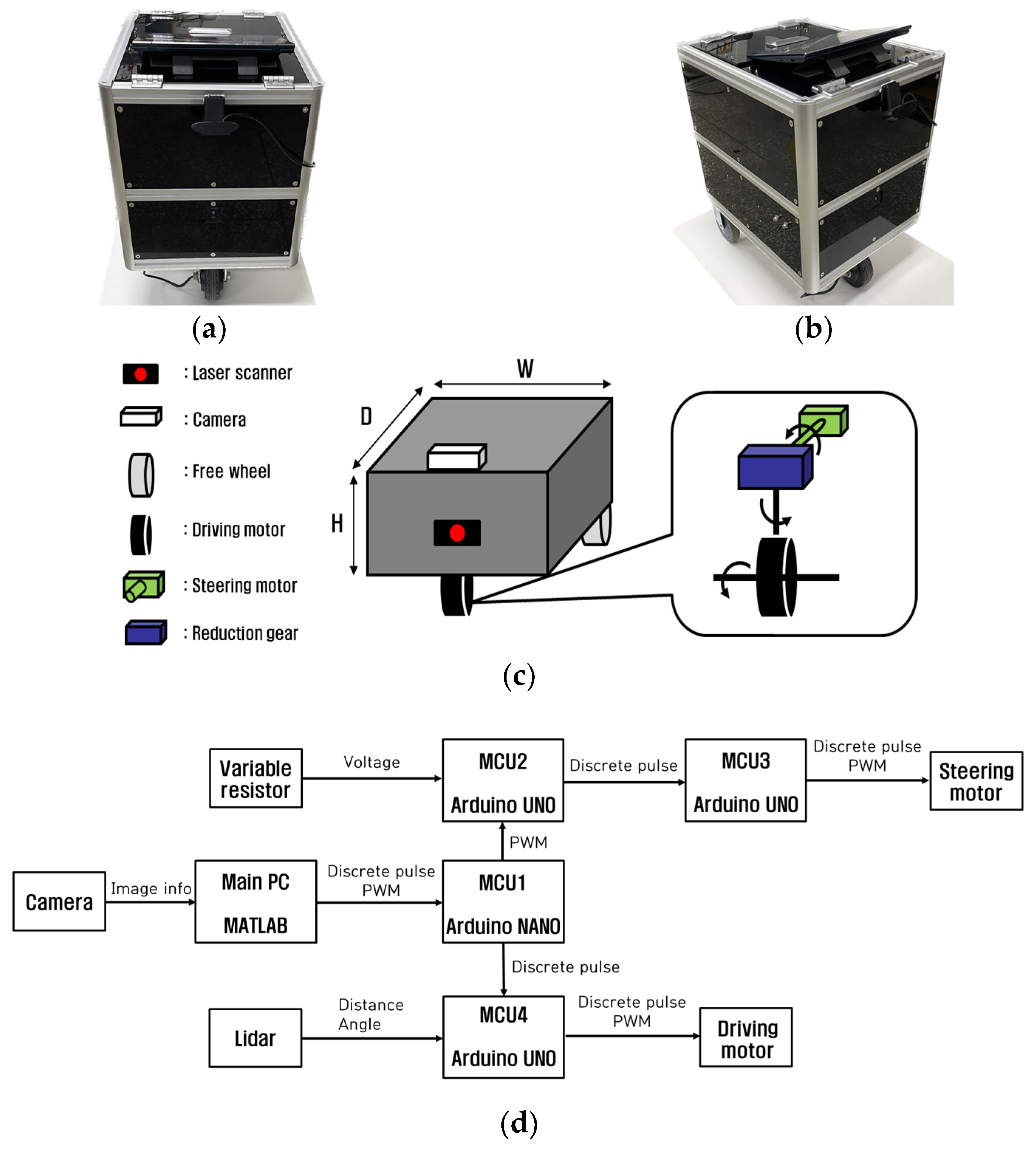
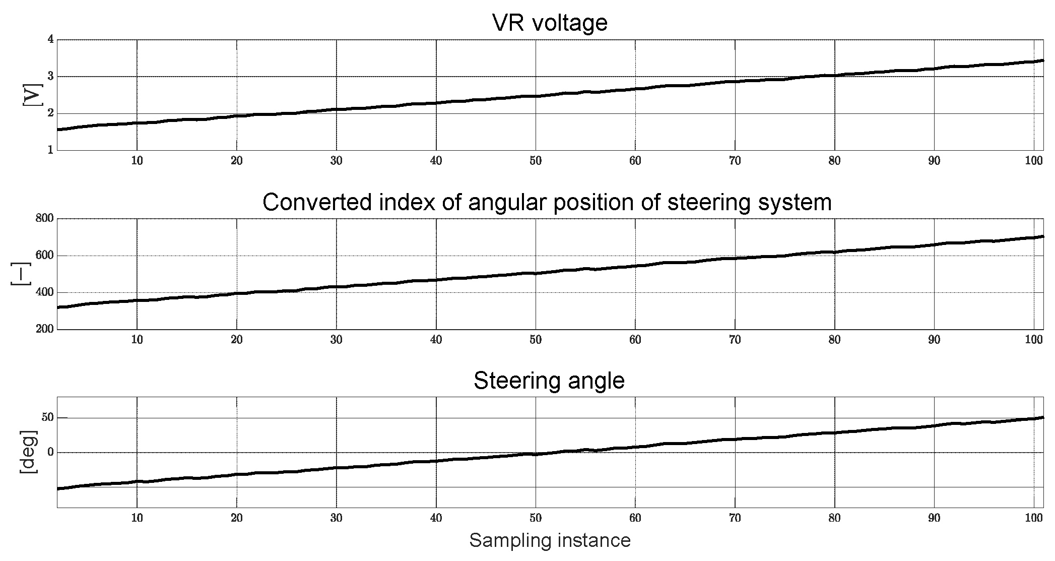
Figure 1 illustrates the comprehensive model schematic of the autonomous mobility path tracking algorithm. In the perception section, control errors and RGB errors were calculated using a camera based on a multi-particle filter. The current steering angle was calculated using a variable resistor (VR), while distance and angle data were measured using lidar to detect obstacles in the surrounding environment. In the decision section, the steering angle error is calculated by using the control errors obtained from the multi-particle filter and the target steering angle derived from the adaptive steering control algorithm. Moreover, based on RGB errors and lidar-based measured distance and angle data, path recognition and obstacle detection were determined. In the control section, a pulse signal was generated to control the direction of the steering motor rotation based on the steering angle error. Additionally, a PWM signal was generated to converge the steering angle error to zero. These signals were then applied to the steering motor. The driving motor was controlled by a driving signal that passed through a functional safety algorithm for driving. Constant PWM signals were applied and traveled at a constant velocity.

Section 2.1 describes a method for deriving control errors using a camera based on a multi-particle filter. In Section 2.2, an adaptive steering control algorithm designed based on a sliding mode approach and weighted injection using control errors and coefficients of simplified error dynamics estimated based on RLS is described.

2.1. Multi-Particle Filter-Based Control Errors Derivation

The particle filter converges towards the RGB value that best matches the camera image by iteratively executing particle update, likelihood calculation, and resampling steps. Equation (1) outlines the procedure for updating the generated particles. It predicts the current particles’ position and speed based on the preceding state value.

$$X_k=X_{k-1}+{\mathrm{w}}_{\mathrm{k}-1}$$

(1)

In Equation (1), the current particles’ positions and velocities $\left(X_k\right)$ are forecasted by adding the discrete-time particles from the previous ($X_{k-1}$), coupled with the system noise sequence ($w_{k-1})$. This noise sequence results from the product of the standard deviation of position and velocity and the disturbance [29].

$$L_{log}=\log \left(\frac{1}{\sqrt{2\pi }{\sigma }_{RGB}}{e}^{\frac{-d^2}{2{\sigma }_{RGB}^2}}\right)$$

(2)

$$d=\sqrt{{\left(R_c-R_t\right)}^2+{\left(G_c-G_t\right)}^2+{\left(B_c-B_t\right)}^2}$$

(3)

$$w_N={\sum }_{i=1}^N\frac{{\mathrm{L}}_{\mathrm{N}}}{\sum L_i}$$

(4)

$${\widehat{X}}_k={\sum }_{i=1}^N{w}_N{X}_{k,i}$$

(5)

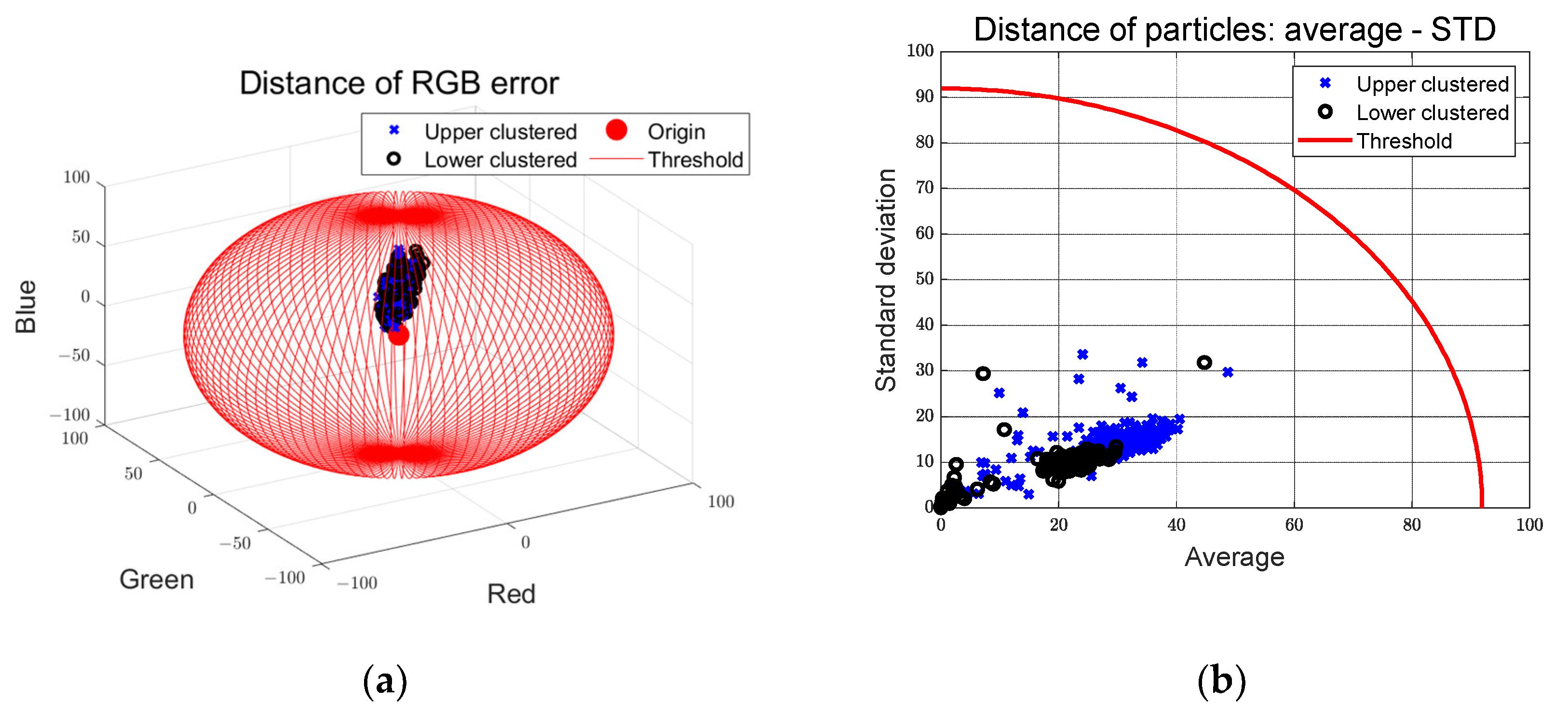
As shown in Equations (2) and (3), the likelihood is calculated using a Multinomial resampling methodology that takes into account the error between the target RGB value and the RGB standard deviation. Particles with a low weight are then replaced by particles with a high weight through weight calculation, as shown in Equation (4). This enables the determination of the predicted location that most closely corresponds to the target RGB, as illustrated in Equation (5). The iterative execution of particle update, likelihood calculation, weight update, and resampling engenders the iterative refinement of the predicted location. 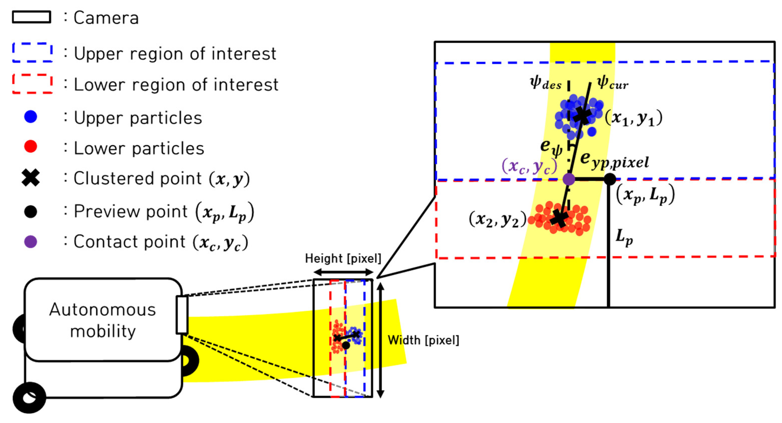Figure 2 presents a schematic illustration of the control error derivation using a multi-particle filter.

Particles within two regions of interest (ROIs), denoted as upper and lower, are generated. Clustering these particles yields two clustering points emanating from the location most akin to the target path RGB. Employing a straight line that intersects the two cluster points and a contact point $\left(x_c,y_c\right)$ perpendicular to the preview point $\left(x_p,y_p\right)$, pixel-based lateral preview error $e_{yp,pixel}$ and current yaw angle error $e_{\psi }$ are derived (Equations (6)–(8)).

$$e_{yp,pixel}=x_c-x_p$$

(6)

$${\psi }_{cur}={\tan }^{-1}\left(\frac{y_2-y_1}{x_2-x_1}\right)$$

(7)

$$e_{\psi }={\psi }_{cur}-{\psi }_{des}$$

(8)

The preview point is designed at the camera’s width midpoint, with preview distance and ROI range being predetermined design parameters. To accommodate camera distortion and perspective, the upper and lower ROIs are set at a 2:1 ratio. The desired yaw angle, as determined through the multi-particle filter for a straight path, approximates zero based on experimental findings. The derived value for the target yaw angle is approximately −0.04 (rad).

2.2. Adaptive Steering Control Algorithm

Figure 3 presents the schematic model illustrating the proposed adaptive steering control algorithm. Multi-particle filter-based control errors are derived using the RGB data from the camera image. The coefficients pertinent to the RLS-based simplified error dynamics are estimated, alongside control errors, by assessing the rate of change in errors obtained through the Kalman filter. The adaptive steering control algorithm, designed based on the sliding mode approach and weighted injection, is responsible for determining the desired steering angle. This algorithm effectively employs both the estimated coefficient and control error.

Equation (9) encapsulates the integrated error achieved by assigning weights to the lateral preview and yaw angle errors, both of which stem from the multi-particle filter. Building upon this foundation, a simplified error dynamics is formulated, as depicted in Equation (10).

$$e=w_1{e}_{yp,pixel}+w_2{e}_{\psi }$$

(9)

$$\dot{e}=Ae+B+u$$

(10)

To deduce the coefficients pertinent to the error dynamics described in Equation (10), RLS with multiple forgetting factors is employed. This method involves the definition of output $\left(y\right)$, regressor $\left(\varphi \right)$, and estimate $\left(\theta \right)$, as outlined in Equations (11) and (12).

$$y=\varphi {\theta }^T, \varphi =\left[\begin{array}{cc}{\varphi }_1& {\varphi }_2\end{array}\right], \theta ={\left[\begin{array}{cc}{\theta }_1& {\theta }_2\end{array}\right]}^T$$

(11)

$$y=\dot{e}(k-1)-u(k-1), \varphi =\left[\begin{array}{cc}e(k-1)& 1\end{array}\right], \theta ={\left[\begin{array}{cc}A\left(k\right)& B\left(k\right)\end{array}\right]}^T$$

(12)

Equation (13) presents a cost function for RLS with multiple forgetting factors that span from zero to one. As the value approaches unity, preceding data is accorded greater weight, thereby instigating gradual parameter estimation changes.

$$\begin{gathered} V\left({\widehat{\theta }}_1\left(k\right),{\widehat{\theta }}_2\left(k\right),k\right)=\frac{1}{2}\sum _{i=1}^k{\lambda }_1^{k-i}{\left(y\left(i\right)-{\varphi }_1\left(i\right){\widehat{\theta }}_1\left(k\right)-{\varphi }_2\left(i\right){\theta }_2\left(k\right)\right)}^2+ \\ \frac{1}{2}\sum _{i=1}^k{\lambda }_2^{k-i}{\left(y\left(i\right)-{\varphi }_1\left(i\right){\theta }_1\left(k\right)-{\varphi }_2\left(i\right){\widehat{\theta }}_2\left(k\right)\right)}^2 \end{gathered}$$

(13)

By leveraging the regressor outlined in Equation (12), the coefficients governing the estimation simplified error dynamics, which minimize the cost function of the recursive least squares method defined in Equation (13), are computed. This process is embodied in Equation (14) [30].

$$\begin{gathered} \left[\begin{array}{c}{\widehat{\theta }}_1\left(k\right)\\ {\widehat{\theta }}_2\left(k\right)\end{array}\right]={\left[\begin{array}{cc}1& L_1\left(k\right){\varphi }_2\left(k\right)\\ L_2\left(k\right){\varphi }_1\left(k\right)& 1\end{array}\right]}^{-1}\times \\ \left[\begin{array}{c}{\widehat{\theta }}_1\left(k-1\right)+L_1\left(k\right)\left(y\left(k\right)-{\varphi }_1\left(k\right){\widehat{\theta }}_1\left(k\right)-{\varphi }_2\left(k\right){\theta }_2\left(k\right)\right)\\ {\widehat{\theta }}_2\left(k-1\right)+L_2\left(k\right)\left(y\left(k\right)-{\varphi }_1\left(k\right){\theta }_1\left(k\right)-{\varphi }_2\left(k\right){\widehat{\theta }}_2\left(k\right)\right)\end{array}\right] \end{gathered}$$

(14)

Within Equation (14), the gain value $\left(L\right)$ for estimation and the covariance $\left(P\right)$, which remains positively oriented, are updated at each sampling instance. This is outlined in Equation (15).

$$\begin{gathered} L_1\left(k\right)=P_1\left(k-1\right){\varphi }_1\left(k\right){\left({\lambda }_1+{{\varphi }_1}^T\left(k\right)P_1\left(k-1\right){\varphi }_1\left(k\right)\right)}^{-1} \\ {P}_1\left(k\right)=\left(I-L_1\left(k\right){{\varphi }_1}^T\left(k\right)\right)P_1\left(k-1\right)/{\lambda }_1 \\ {L}_2\left(k\right)=P_2\left(k-1\right){\varphi }_2\left(k\right){\left({\lambda }_2+{{\varphi }_2}^T\left(k\right)P_2\left(k-1\right){\varphi }_2\left(k\right)\right)}^{-1} \\ {P}_2\left(k\right)=\left(I-L_2\left(k\right){{\varphi }_2}^T\left(k\right)\right)P_2(k-1)/{\lambda }_2 \end{gathered}$$

(15)

To assess the stability of the control algorithm and devise the control input, an A Lyapunov candidate function is introduced, as shown in Equation (16). The integrated error is factored into this process. Equation (17) lays out two conditions for the Lyapunov candidate function and its derivative, ensuring the integrated error’s convergence to zero within a finite time.

$$J=\frac{1}{2}{e}^2$$

(16)

$$\begin{gathered} Condition (1) \dot{J}\le -\alpha V^{\frac{1}{2}}, \alpha >0 \\ Condition (2) \underset{\left|e\right|\to \infty }{\lim }V=\infty \end{gathered}$$

(17)

To ascertain the magnitude of the injection term required to expedite the integrated error’s convergence to zero within a finite duration, the integrated error’s rate of change, defined in Equation (10), can be substituted for the time derivative of the Lyapunov candidate function. This leads to the representation shown in Equation (18).

$$\dot{J}=e\dot{e}=e\left(Ae+B+u\right)$$

(18)

The control input, devised to minimize errors and ensure control stability, is defined in Equation (19). Within this equation, coefficients of the simplified error dynamics are estimated using RLS, and the injection term is established using integrated error, as denoted in Equation (20).

$$u=-\widehat{A}e-\widehat{B}+\nu$$

(19)

$$\nu =-\rho sign\left(e\right)$$

(20)

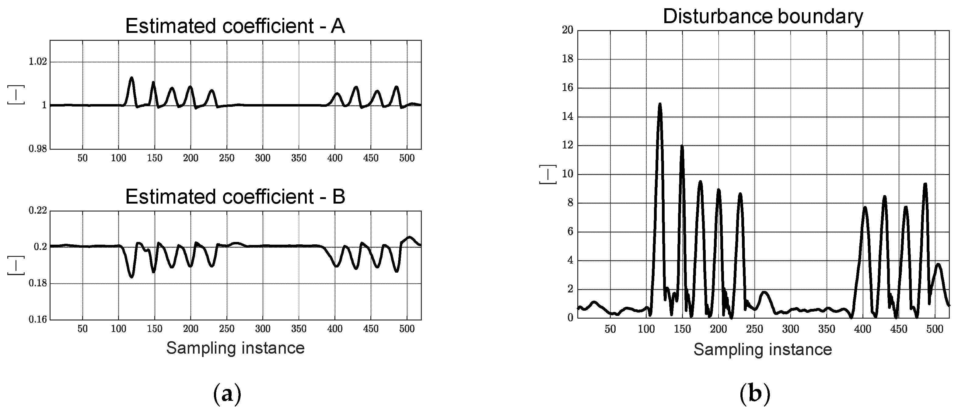
Substituting Equations (19) and (20) into the derivative of the Lyapunov candidate function results in the formulation depicted in Equation (21). The disparity between the actual system and the estimated value is represented as demonstrated in Equation (22). The scope of the disturbance boundary can be characterized using the reachability factor, as expounded upon in Equations (23) and (24).

$$\dot{J}=e\left(Ae+B-\widehat{A}e-\widehat{B}+\nu \right)=e\left(\left(A-\widehat{A}\right)e+\left(B-\widehat{B}\right)-\rho sign\left(e\right)\right)$$

(21)

$$r=\left(A-\widehat{A}\right)e+\left(B-\widehat{B}\right)$$

(22)

$$\left|r\right|+\eta =L_b$$

(23)

$$\left|r\right|\le L_b$$

(24)

By substituting the disturbance’s boundary, as compliant with Equation (24), into Equation (21), it can be expressed as Equation (25). Furthermore, by leveraging convergence condition 1 within a finite time, it can also be represented as Equation (26).

$$\dot{J}=e\left(r+\nu \right)\le \left|e\right|L_b-\left|e\right|\rho =-\left|e\right|(\rho -L_b)$$

(25)

$$\dot{J}\le -\alpha V^{\frac{1}{2}}=-\frac{\alpha }{\sqrt{2}}\left|e\right|$$

(26)

When the right-hand sides of Equations (25) and (26) are equated, the injection term’s magnitude can be determined using Equation (27).

$$\rho =\frac{\alpha }{\sqrt{2}}+L_b$$

(27)

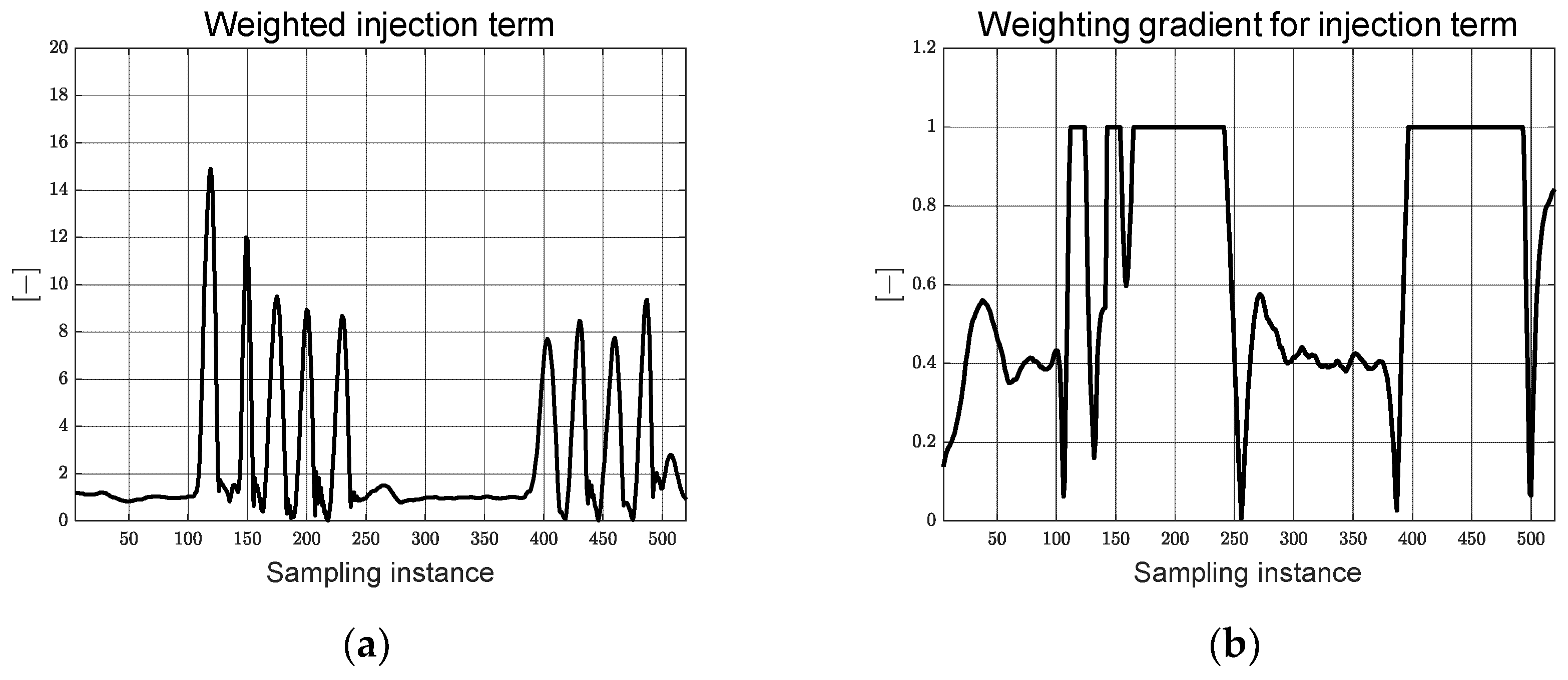
The weighted injection term’s magnitude is defined as per Equation (28), with the weighting factor $\left(m\right)$ ranging from zero to one. The weighting factor is designed using the absolute integrated error value and threshold for the integrated error ($e_{th}$), as elucidated in Equation (29). Where the threshold in Equation (29) is a design parameter used to adjust the gradient of the weighting factor. When the absolute value of the integrated error is smaller than the threshold, the weighting factor is computed by a linear function of less than one, which significantly impacts the finite time convergence condition. Conversely, when the absolute value of the integrated error is larger than the threshold, the weighting factor is set to a value of one. This ensures swift convergence to zero during instances of significant control error by modulating the injection term’s magnitude based on the error’s magnitude while adhering to the finite time convergence condition.

$$\rho =\frac{\alpha }{\sqrt{2}}\left(1-m\right)+m\left(\left|r\right|+\eta \right)$$

(28)

$$m=\frac{\left|e\right|}{e_{th}}, \left(\left|e\right|\ge {\mathrm{e}}_{th},m=1\right)$$

(29)

By constructing a Lyapunov candidate function grounded in a sliding mode approach and weighted injection, an adaptive steering control input is derived. Equation (30) showcases the derivation of the control input employing control errors and coefficients of the simplified error dynamics, as estimated through RLS. To mitigate the chattering phenomenon induced by the sign function, a sigmoid function is employed. When Equation (30) is integrated into Equation (18), which represents the Lyapunov function’s derivative, it yields Equation (31). This underlines that the algorithm’s Lyapunov stability is established based on the designed weighted injection term.

$$u=-\widehat{A}e-\widehat{B}-\rho sign\left(e\right)$$

(30)

$$\dot{J}=-\left|e\right|\frac{\alpha }{\sqrt{2}}\left(1-m\right)+m\left(\left|r\right|+\eta \right)<0, (e\ne 0)$$

(31)

The ensuing section delves into the performance evaluation outcomes of the adaptive steering control algorithm, anchored in actual autonomous mobility.

3. Performance Evaluation

To evaluate the proposed adaptive steering control algorithm, a simplified error equation based on a multi-particle filter and sliding modes was utilized. This approach eliminates the need for a mathematical model and camera calibration. The evaluation was conducted on the actual autonomous mobility developed, using S-curved and elliptical path tracking performance evaluation. The adaptive steering control algorithm was implemented in a MATLAB environment.

3.1. Design of Autonomous Mobility Platform

Figure 4 shows the front view, side view, concept, and hardware architecture of the developed autonomous mobility. Autonomous mobility consists of a single steering and driving system equipped with a camera, lidar sensor, VR, and two free wheels. The lidar detects surrounding obstacles, and the camera is used for path tracking based on multi-particle filters. VR calculates the angle of the current steering motor. The steering control operates by applying PWM and pulse to the steering motor to minimize the error between the desired steering angle, determined using adaptive steering control, and the current steering angle calculated based on VR. The goal is to make the error converge to zero. Additionally, a pulse signal is applied in the rotation direction based on the sign of the steering angle error to allow for steering and path tracking. The driving control operates at a constant speed by applying a constant PWM signal to the driving motor. Driving and braking actions are performed by applying a pulse signal based on the driving flag derived from lidar and multi-particle filter-based functional safety algorithms. Since the particle filter follows a path based on the principle of moving towards the point that is most similar to the target RGB based on probability, it is necessary to determine the error in target path recognition. The functional safety algorithm applied for this purpose was designed using upper and lower clustered points and other particles derived from multi-particle filters. This algorithm is used to determine target path recognition errors and detect obstacles in the surrounding environment. The error in target path recognition is determined by comparing the distance between the cluster point defined in Equation (3) and the target RGB value error and the distance between the cluster point and other particles, as shown in Equation (32), based on the designed threshold. Here, ${\mu }_{particles}$ and ${\sigma }_{particles}$ represent the average and standard deviation of the distance between the clustered point and other particles, respectively.

$$e_{f.s}=\sqrt{{\mu }_{particles}^2+{\sigma }_{particles}^2}$$

(32)

As can be seen in Figure 4d, the developed autonomous mobility system utilized one main PC and four Micro Control Units (MCUs) to control the driving and steering motors, as well as to measure serial communication-based sensor data from lidar and VR. Using a main PC equipped with an Intel Core i7-1195 CPU, we implemented a multi-particle filter algorithm by connecting the main PC to a camera in the MATLAB environment. The desired steering angle, calculated by the main PC, is transmitted to MCU2 through MCU1 using a PWM signal. The steering angle error was calculated by comparing the current between the steering angle calculated based on VR and the reference value. The steering angle error is transmitted to MCU3 using a discrete pulse signal to control the steering motor. In addition, the driving signal generated by the functional safety algorithm in the main PC is transmitted to MCU4 through MUC1 using a discrete pulse signal to control the driving motor. The clock frequency of the MCUs is 16 MHz, and the MCUs are configured in a distributed structure with three Arduino UNOs and one Arduino NANO operating at 5 V. The four MCUs used a 6 V battery, while the steering and driving motors were powered by two 24 V batteries. In addition, Ublox’s GPS was used to confirm the trajectory of the autonomous mobility, while RTK was applied to acquire data at a frequency of 8 Hz.

Table 1. Autonomous mobility and camera specifications.

Parameter	Unit	Value
Mass $\left(M\right)$	kg	About $38.6$
Height $\left(H\right)$	m	$0.45$
Depth $\left(D\right)$	m	$0.55$
Width $\left(W\right)$	m	$0.45$
Wheel base $\left(L\right)$	m	0.5
Wheel tread $\left(t_w\right)$	m	0.375
Resolution of camera	pixel	$1280\times 720$

presents the specifications of the developed autonomous mobility and the resolution of the camera utilized in the experiment. The mass of the autonomous mobility is relatively small, about 38.6 kg.

The steering angle was determined by translating the VR voltage into a converted index value that reflects the angular position of the steering system, as illustrated in Equation (33). Within Equation (33), ‘$A_{VR}$’ denotes the converted index value of the angular position, which spans from 0 to 1023, while ‘$V_{VR}$’ signifies the VR voltage, which spans from 0 to 5 V. Figure 5 visualizes the VR voltage and the converted index of angular position as the steering angle changes from −50 to 50 degrees.

$$\begin{gathered} {\delta }_{cur}=0.2685\times A_{VR}-138.0615 \\ Where, A_{VR}=V_{VR}\times \frac{1023}{5} \end{gathered}$$

(33)

3.2. S-Curved Path Tracking Scenario

In this section, an assessment of the adaptive steering control algorithm was conducted within an S-curved path scenario. The designated path was delineated by yellow color bands, encompassing two semicircles, each with a 2 m radius, as depicted in Figure 6. The intended path was devoid of any obstructions within its vicinity. The design parameters for both the adaptive steering control algorithm and the multi-particle filter are detailed in

Table 2. Design parameters of the multi-particle filter and adaptive steering control.

Parameter	Unit	Value
Standard deviation of position $\left({\sigma }_{pos}\right)$	-	$20$
Standard deviation of velocity $\left({\sigma }_{vel}\right)$	-	$25$
Standard deviation of RGB $\left({\sigma }_{RGB}\right)$	-	$20$
The number of particles $\left(N\right)$	-	$1000$
RGB of target path $\left(r_t,g_t,b_t\right)$	-	$\left(254, 252, 164\right)$
Threshold of RGB data error	-	$100$
Threshold of standard deviation and average of RGB distance	-	$\left(65, 65\right)$
ROI of upper particle	pixel	$200<H_{pixel}<300$
ROI of lower particle	pixel	$300<H_{pixel}<350$
Preview point $\left(x_p, L_p\right)$	pixel	$\left(640, 300\right)$
Weightings of control error $\left(w_1, w_2\right)$	-	$\left(0.028, 1.2\right)$
Integrated error threshold $\left(e_{th}\right)$	-	$4$
Decay rate of the Lyapunov function $\left(\alpha \right)$	-	$1.8$
Reachability factor $\left(\eta \right)$	-	$0.01$
Initial value of estimated states $\left({\widehat{\theta }}_1, {\widehat{\theta }}_2\right)$	-	$\left(1, 0.2\right)$
Forgetting factor $\left({\lambda }_1, {\lambda }_2\right)$	-	$\left(0.998, 0.998\right)$

. These identical parameters were employed for the execution of both the S-curved and elliptical scenarios. These parameters were determined using the trial-and-error method.

Figure 7 displays four frames derived from real experiments, offering a visual representation of the multi-particle filter’s execution. Where, green and purple dots represent upper and lower particles, and black dots indicate clustered points. Furthermore, Figure 8 presents four frames showcasing the environmental conditions during the experiments. The observations made from Figure 7 affirm that particles within the ROI, established at a 2:1 ratio, gather along the desired path. Both Figure 7 and Figure 8 reveal a coherent pursuit of the target RGB tracking through the multi-particle filter and the desired path through adaptive steering control.

Figure 9 illustrates the control error acquired from the multi-particle filter, the integrated error computed through control error weighting, and the estimated integrated error differential derived from the Kalman filter. The converted lateral preview error in Figure 9 shows the result of converting pixels to actual distances. To convert to the actual distance of lateral preview distance, 15 cm rulers were placed at 20 cm intervals, and the actual distance for each pixel was measured through an experiment. Accordingly, a function to convert the lateral preview error based on camera pixels to the actual distance was experimentally derived, as shown below in Equation (34), and the function consists of preview distance and pixel-based lateral preview error.

$$e_{yp} \left[m\right]=(\left(-0.0001L_p+0.0976\right)\times e_{yp,pixel})/100$$

(34)

As can be seen from the integrated error, the symmetric nature of the control error’s fluctuation, both in the positive and negative directions, is evident due to the S-curved path. Moreover, the phenomenon of control error oscillation during curved driving is discernible. This oscillation can be attributed to factors such as data communication between the MCU and the main PC, the discrete pulse signals, and the fixed ROI.

Figure 10a exhibits the real-time derived coefficients A and B of the simplified error dynamics through RLS, and Figure 10b presents the computed disturbance boundary based on the residual between the actual system and its estimated system. In Figure 11, the weighted injection is depicted, considering finite-time convergence conditions and the disturbance boundary with the integrated error’s magnitude. Notably, as the integrated control error fluctuates in both directions, the estimated RLS-based coefficients display analogous fluctuations. This correspondence in behavior leads to observable variations in the magnitude of the weighted injection based on the integrated error’s magnitude.

Figure 12a displays the desired steering angle derived from the adaptive steering control algorithm alongside the present steering angle computed from VR. Figure 12b presents the steering angle error. Figure 13a showcases the clockwise and counterclockwise rotation flags used for discerning the rotation direction predicated on the steering angle error’s status. In this paper, the threshold value of the steering angle error is set to 0 degrees. As a result, excessive rotation steering pulse signals are applied to the steering motor, leading to unnecessary energy consumption. In order to maintain reasonable path tracking performance and improve energy efficiency in the future, we plan to reduce the rotational steering flag ratio by applying a threshold value for the steering angle error. Within Figure 13b, a driving flag of one signifies the implementation of consistent-speed driving, achieved by applying a specific PWM to the driving motor. Conversely, a driving flag of zero corresponds to a braking arrangement activated through a pulse signal. Notably, because there are no obstacles within the target path and the surrounding environment, the driving signal remains at one. As observed in Figure 12 and Figure 13, the desired steering angle is tracked by applying PWM and pulse to the steering motor based on the steering angle error. Vibration phenomena can be observed at the desired steering angle determined by the adaptive steering control algorithm. This confirms that the oscillation phenomenon of the control error, which is derived based on the aforementioned particle filter, also affects control performance. In the future, it is expected that the vibration phenomenon at the desired steering angle will be alleviated through algorithm improvements in the perception section, specifically in the control error derivation process.

Figure 14 presents the distance between the cluster and other particles alongside the multi-particle filter-induced RGB error pertaining to a functional safety algorithm. Given the absence of obstructions along the target path, it is evident that both the RGB error and particle spacing adhere to the specified threshold. Moving to Figure 15, normal driving is observable, devoid of particle filters and lidar-identified obstacles, as evident in the depicted sampling instances.

Figure 16a displays the trajectory of the autonomous mobility utilizing Ublox’s GPS alongside the waypoint trajectory gauged through several walks along the generated path. In the future, we plan to determine lateral errors by conducting experiments in a controlled environment using reasonable GPS data measurements. Meanwhile, Figure 16b delineates an experimental duration of approximately 60 s, with a loop cycle time averaging around 0.229 s per individual sampling instance.

3.3. Elliptical Path Tracking Scenario in Working Environment

In various industrial sites, obstacles or workers may be present in the target path due to the complex surrounding environment, including items and workers. When such obstacles or workers exist, braking or avoidance is necessary for worker safety, work efficiency, and convenience. Accordingly, in this section, a scenario has been executed to augment work efficiency and offer convenience to workers in diverse fields, such as smart farms and smart factories. As shown in Figure 17, autonomous mobility presents obstacle and worker in black squares contrasting with the target path within an elliptical trajectory, encompassing two 5 m straight segments and two semicircles with a 2 m radius. In this paper, autonomous mobility was designed to brake in the presence of obstacles or workers. Therefore, this scenario shows not only the results of elliptical path tracking but also the results of functional safety algorithms to ensure the convenience and safety of workers when they load autonomous mobility or when obstacles are present.

Figure 18 is the image of the multi-particle filtering; the 135th frame demonstrates the particles deviating from the path due to the presence of an obstacle. Where, green and purple dots represent upper and lower particles, and black dots indicate clustered points. Additionally, in the 310th frame, it is apparent that the autonomous mobility is braking, even though particles have converged on the target path. This response is attributed to the detection of a worker using lidar while loading items onto the autonomous mobility. Figure 19 offers a snapshot from the experimental video, affirming that the braking is performed by the functional safety algorithm when the obstacle and worker are present in the target path.

As shown in Figure 20a, the yaw angle error, attributed to obstacles in the target path, experiences rapid changes at approximately 135 sampling instances. In addition, it is noticeable that control errors and oscillation occur due to driving on curved roads, sampling instances at 100 to 200 and 380 to 520. In Figure 20b, the integrated control remains within the threshold in the positive as it follows the counterclockwise path along the elliptical track. As shown in Figure 21 and Figure 22, the control error increases in the curved section. This results in an increased magnitude of the weighted injection. Accordingly, when the integrated error exceeds the threshold, the weighting factor becomes one, and the control input is determined by considering the disturbance boundary derived from the estimated residual A and B based on RLS.

At approximately 135 and 300 sampling instances, the functional safety algorithm detects the obstacle and worker in the target path, causing the autonomous mobility to brake. This transition is reflected in the alteration of the driving flag from one to zero. Even in the state of braking, as particles continue their movement, the control error may experience rapid fluctuations in either direction. In this way, since the adaptive steering control utilizes the control error derived from the particle filter, when there is a misjudgment in path recognition, the control input is also miscalculated. As a result, as shown in Figure 23a, displaying the current steering angle, a mechanism has been devised to guide the current steering angle to zero to avert deviation from the path misjudgments in path recognition. Additionally, Figure 24a shows that rotational steering flag changes to zero.

Depicted in Figure 25 is the influence of an obstacle in the target path, resulting in an increase in the distance between the clustered point and the target path RGB error at approximately 130 sampling instances, surpassing the predefined threshold. Notably, the distance between the clustered point and the other particles remains within the set threshold. This indicates the convergence of particles to a location distinct from the target path. When either the RGB error distance or the relative distance of the particles equals or surpasses the threshold value, this is recognized as a misjudgment in path recognition. Correspondingly, Figure 26 illustrates the transition of the driving flag from one to zero. This shift occurs due to obstacle detection along the target path based on the RGB error distance at approximately 130 sampling instances, followed by worker detection through lidar at approximately 300 sampling instances. As can be seen in Figure 25 and Figure 26, when obstacles or workers exist within the target path, the braking performance can be verified to ensure worker safety and facilitate convenience using the functional safety algorithm. The trajectory of the GPS-based autonomous mobility, aligned with waypoints, is showcased in Figure 27. Resembling a semicircle with two 5 m straight segments and two 2 m radii, this trajectory captures the essence of the path. Furthermore, the experimental time amounted to approximately 130 s, with the loop cycle taking approximately 0.227 s.

4. Discussion

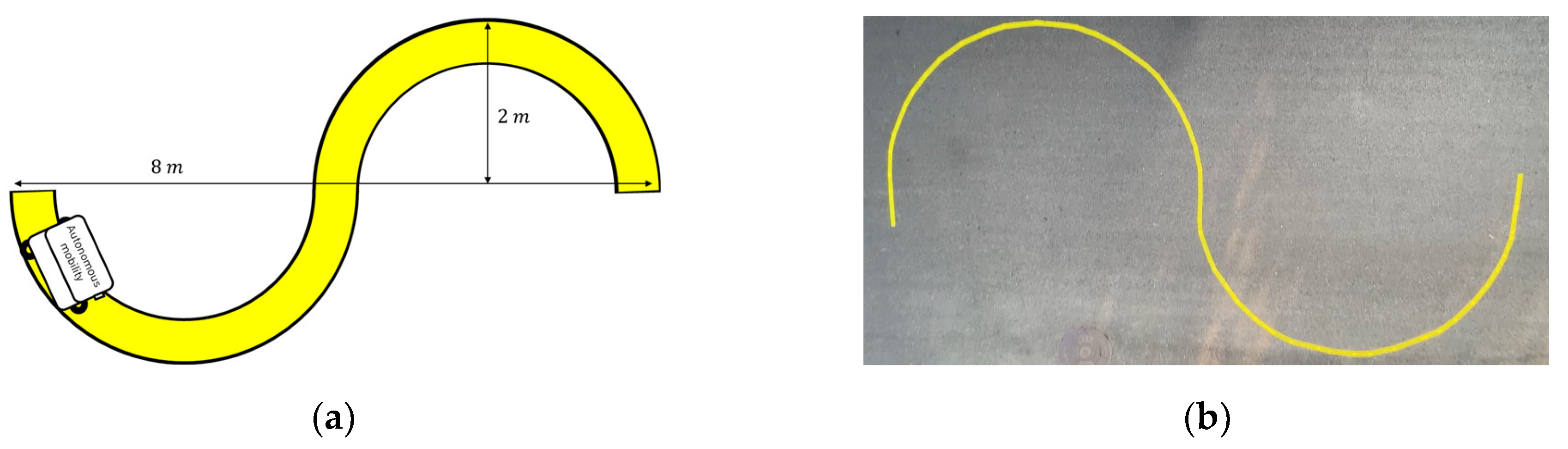
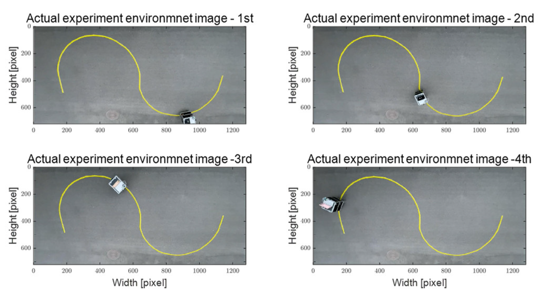
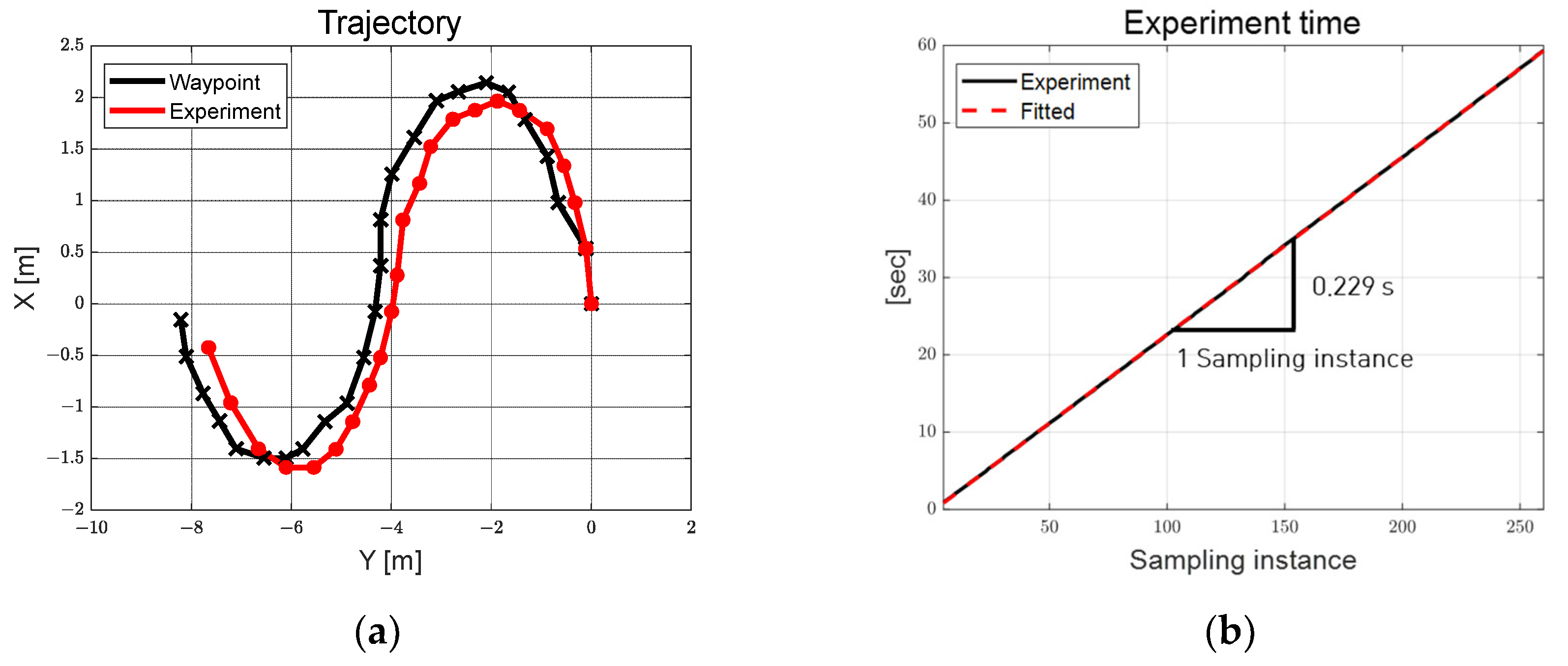
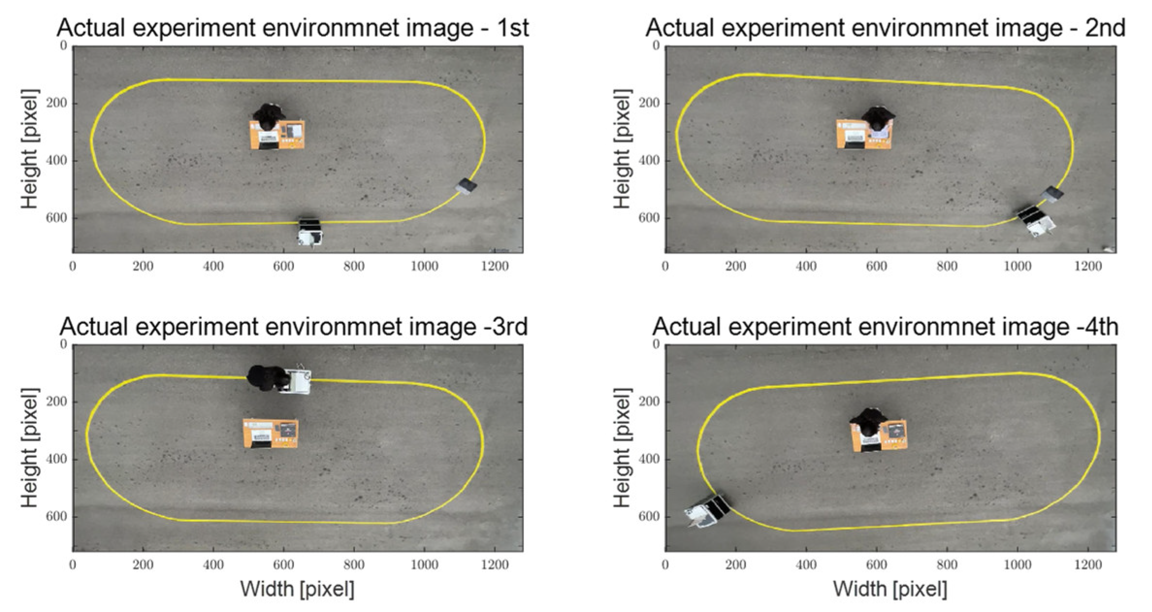
The performance of the adaptive steering control algorithm, as proposed in this study, was assessed using a single steering and driving system consisting of autonomous mobility. Evaluation scenarios encompass two distinct environments: an obstacle- and worker-free S-curved path and an elliptical path with obstacles and workers. These scenarios are designed to portray the utilization of autonomous platforms, catering to improve work efficiency and enhance worker convenience across diverse sectors, including smart farms and smart factories. The evaluation results confirm a reasonable path tracking performance of the adaptive steering control input, derived through multi-particle filter-based control error and coefficients estimated in real-time through RLS.

Since RLS-based coefficient estimation is sensitive to the initial value parameter setting, it was determined using the trial-and-error method. Additionally, the control error derivation in the recognition and the steering control process confirmed the oscillation phenomenon. This is expected to be the motion in the particle filtering process, the discrete signal of the rotation direction applied to the steering motor consisting of zero and one, and the signal processing process between the four MCUs and the main PC. The autonomous mobility used in this study traveled at a low speed of approximately 0.25 m/s, applying a constant PWM to the driving motor. With its relatively low mass of approximately 38.6 kg, the mobility exhibited reasonable path tracking outcomes even when experiencing oscillations. Nevertheless, it should be noted that such oscillations might potentially impact path tracking performance during high-speed operation. Addressing this concern is a goal for future work, potentially involving the utilization of filtering techniques like RLS and the Kalman filter to compute control errors, as well as smooth and fast signal processing between the MCUs and the main PC.

In addition, because the algorithm proposed in this paper relies on RGB images, changes in lighting conditions may affect the performance of the control. Since the control error is derived from tracking the RGB values of the target path using a particle filter, any sudden change in lighting requires modification of the particle filter parameters. Accordingly, the performance evaluation of the algorithm proposed in this paper was conducted between 6 and 8 PM, when sunlight does not have much influence. The average RGB values for scenarios 1 and 2 are shown in

Table 3. Average of RGB value at performance evaluation.

Division	Scenario 1	Scenario 2
Average of red value	128	140
Average of green value	126	129
Average of blue value	148	135

. In the future, we plan to enhance the algorithm by incorporating average RGB values to robustly detect the target path, even in varying lighting conditions.

5. Conclusions

In this paper, we propose an adaptive steering control algorithm employing a sliding mode approach and a weighted injection term. The multi-particle filter-based control error using a camera was derived, and simplified error dynamics based on integrated control were defined by applying weighting factors to the control error. We estimate the coefficients for this error dynamics using RLS with multiple forgetting factors. The adaptive steering control input is then formulated by designing a cost function that incorporates the weighted injection term and sliding mode approach using the control errors and estimated coefficients.

The objective of this study is to achieve path tracking steering control for autonomous mobility platforms, overcoming the complexity-induced uncertainty of mathematical models seen in the development of diverse autonomous systems. The adaptive steering control input can be determined using the control error derived from pixel via a multi-particle filter, avoiding reliance on mathematical model parameters. This is achieved by estimating coefficients of the simplified error dynamics using real-time RLS. Furthermore, by incorporating a weighted injection term that adjusts according to the control error’s magnitude, the adaptive control input capable of rapidly reducing the control error to zero is attained while adhering to finite time convergence conditions.

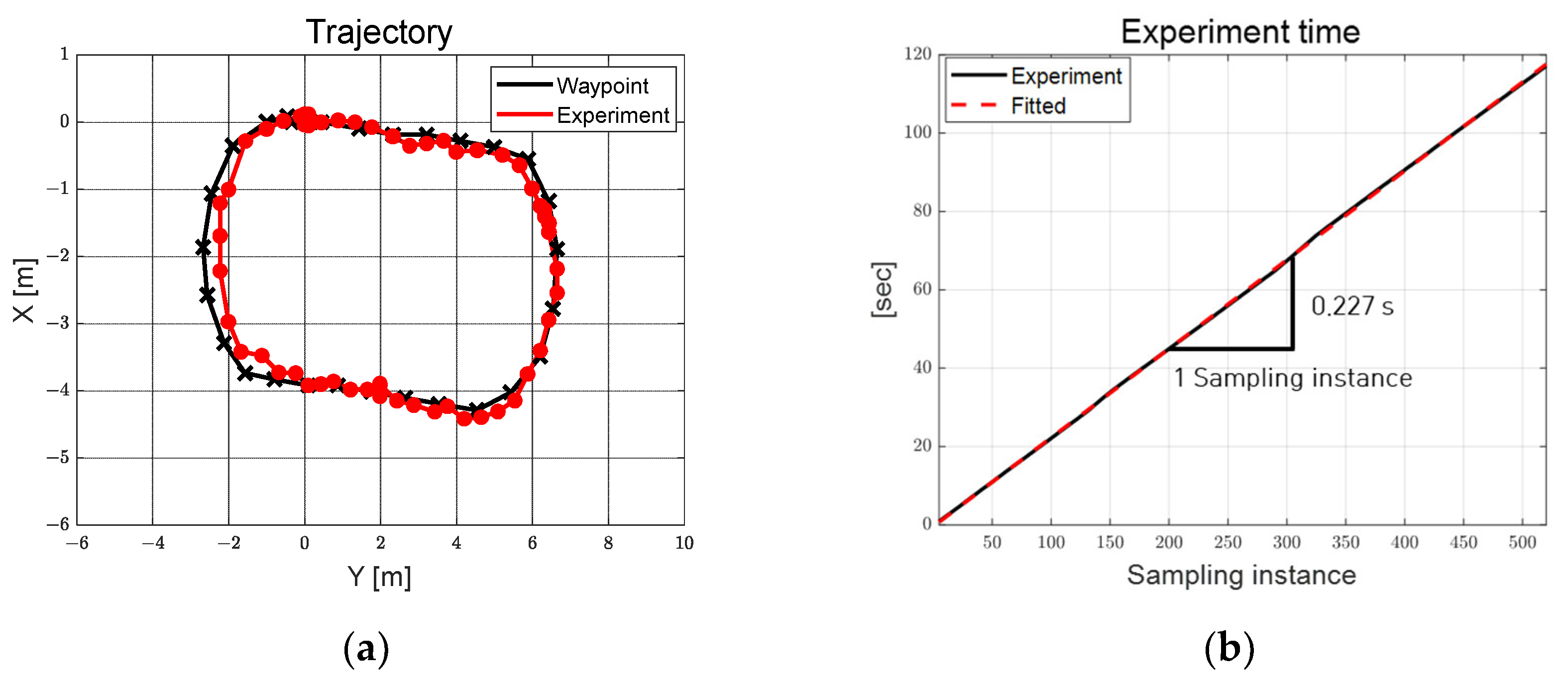
The multi-particle filter and RLS-based adaptive path tracking algorithm were implemented in the MATLAB environment and evaluated using actual autonomous mobility. As a result of the evaluation, it was confirmed that the proposed adaptive steering control algorithm demonstrated reasonable path tracking performance on an S-curved path without obstacles and an elliptical path with obstacles. On average, the algorithm took 0.228 s per sampling instance. Furthermore, by implementing a functional safety algorithm, we have confirmed the potential for utilizing autonomous mobility that enhances work safety, efficiency, and worker convenience in diverse industries. However, an oscillation was observed as a result of the particle filtering process used to derive the control error, the signal processing between the four MCUs and the main PC, the discrete pulse signals applied to the steering motor and the steering control process.

In the future, we intend to assess scenarios at varying speeds and paths, aiming to enhance data and signal processing through software and hardware enhancements to minimize oscillations phenomenon in the derivation of control errors and steering control process. Through the software and hardware advancements, it is anticipated that the proposed perception and control algorithms can be effectively applied to path tracking of autonomous mobility platforms in various other applications, such as autonomous vehicles and robots, for active collaboration with human workers.

References

1. Zhang, X.; Zhu, X. Autonomous path tracking control of intelligent electric vehicles based on lane detection and optimal preview method. Expert Syst. Appl. 2019, 121, 38–48. [Google Scholar] [CrossRef]
2. Muthalagu, R.; Bolimera, A.; Kalaichelvi, V. Lane detection technique based on perspective transformation and histogram analysis for self-driving cars. Comput. Electr. Eng. 2020, 85, 106653. [Google Scholar] [CrossRef]
3. Jiao, X.; Yang, D.; Jiang, K.; Yu, C.; Wen, T.; Yan, R. Real-time Lane detection and tracking for autonomous vehicle applications. Proc. Inst. Mech. Eng. Part D J. Automob. Eng. 2019, 233, 2301–2311. [Google Scholar] [CrossRef]
4. Miyamoto, R.; Nakamura, Y.; Adachi, M.; Nakajima, T.; Ishida, H.; Kojima, K.; Kobayashi, S. Vision-based road-following using results of semantic segmentation for autonomous navigation. In Proceedings of the 2019 IEEE 9th International Conference on Consumer Electronics, Berlin, Germany, 8–11 September 2019; pp. 174–179. [Google Scholar]
5. de Morais, G.A.; Marcos, L.B.; Bueno, J.N.A.; de Resende, N.F.; Terra, M.H.; Grassi, V., Jr. Vision-based robust control framework based on deep reinforcement learning applied to autonomous ground vehicles. Control Eng. Pract. 2020, 104, 104630. [Google Scholar] [CrossRef]
6. Khan, M.A.M.; Haque, M.F.; Hasan, K.R.; Alajmani, S.H.; Baz, M.; Masud, M.; Nahid, A. LLDNet: A Lightweight Lane Detection Approach for Autonomous Cars Using Deep Learning. Sensors 2022, 22, 5595. [Google Scholar] [CrossRef] [PubMed]
7. Tsai, T.H.; Yao, C.H. A robust tracking algorithm for a human-following mobile robot. IET Image Process. 2021, 15, 786–796. [Google Scholar] [CrossRef]
8. Han, D.; Peng, Y. Human-following of mobile robots based on object tracking and depth vision. In Proceedings of the 2020 3rd International Conference on Mechatronics, Robotics and Automation, Shanghai, China, 16–18 October 2020; pp. 105–109. [Google Scholar]
9. Matraji, I.; Al-Wahedi, K.; Al-Durra, A. Higher-order super-twisting control for trajectory tracking control of skid-steered mobile robot. IEEE Access 2020, 8, 124712–124721. [Google Scholar] [CrossRef]
10. Moudoud, B.; Aissaoui, H.; Diany, M. Robust trajectory tracking control based on sliding mode of Differential Driving Four-Wheeled Mobile Robot. In Proceedings of the 2020 IEEE 6th International Conference on Optimization and Applications, Beni Mellal, Morocco, 20–21 April 2020; pp. 1–5. [Google Scholar]
11. Fnadi, M.; Plumet, F.; Benamar, F. Model predictive control based dynamic path tracking of a four-wheel steering mobile robot. In Proceedings of the 2019 IEEE/RSJ International Conference on Intelligent Robots and Systems, Macau, China, 3–8 November 2019; pp. 4518–4523. [Google Scholar]
12. Bai, G.; Liu, L.; Meng, Y.; Luo, W.; Gu, Q.; Wang, J. Path tracking of wheeled mobile robots based on dynamic prediction model. IEEE Access 2019, 7, 39690–39701. [Google Scholar] [CrossRef]
13. AL Khatib, E.I.; Jaradat, M.A.K.; Abdel-Hafez, M.F. Low-cost reduced navigation system for mobile robot in indoor/outdoor environments. IEEE Access 2020, 8, 25014–25026. [Google Scholar] [CrossRef]
14. Kim, D.H.; Kim, S.B. Path following control of automated guide vehicle using camera sensor. In Proceedings of the AETA 2018-Recent Advances in Electrical Engineering and Related Sciences, Ostrava, Czech Republic, 11–13 September 2018; pp. 932–938. [Google Scholar]
15. Moghaddasi, S.S.; Faraji, N. A hybrid algorithm based on particle filter and genetic algorithm for target tracking. Expert Syst. Appl. 2020, 147, 113188. [Google Scholar] [CrossRef]
16. Nenavath, H.; Ashwini, K.; Jatoth, R.K.; Mirjalili, S. Intelligent trigonometric particle filter for visual tracking. ISA Trans. 2022, 128, 460–476. [Google Scholar] [CrossRef]
17. Wang, Y.; Wang, X.; Shan, Y.; Cui, N. Quantized genetic resampling particle filtering for vision-based ground moving target tracking. Aerosp. Sci. Technol. 2020, 103, 105925. [Google Scholar] [CrossRef]
18. Xiao, F.; Wu, Q.; Huang, H. Single-scale siamese network based RGB-D object tracking with adaptive bounding boxes. Neurocomputing 2021, 451, 192–204. [Google Scholar] [CrossRef]
19. Grami, T.; Tlili, A.S. Indoor mobile robot localization based on a particle filter approach. In Proceedings of the 2019 19th International Conference on Sciences and Techniques of Automatic Control and Computer Engineering, Sousse, Tunisia, 24–26 March 2019; pp. 47–52. [Google Scholar]
20. Ismail, K.; Liu, R.; Zheng, J.; Yuen, C.; Guan, Y.L.; Tan, U.X. Mobile robot localization based on low-cost LTE and odometry in GPS-denied outdoor environment. In Proceedings of the 2019 IEEE International Conference on Robotics and Biomimetics, Dali, China, 6–8 December 2019; pp. 2338–2343. [Google Scholar]
21. Gareis, M.; Fenske, P.; Carlowitz, C.; Vossiek, M. Particle filter-based SAR approach and trajectory optimization for real-time 3D UHF-RFID tag localization. In Proceedings of the 2020 IEEE International Conference on RFID, Orlando, FL, USA, 28 September–16 October 2020; pp. 1–8. [Google Scholar]
22. Hu, C.; Wang, Z.; Taghavifar, H.; Na, J.; Qin, Y.; Guo, J.; Wei, C. MME-EKF-based path-tracking control of autonomous vehicles considering input saturation. IEEE Trans. Veh. Technol. 2019, 68, 5246–5259. [Google Scholar] [CrossRef]
23. Chen, M.; Ren, Y.; Ou, M. Adaptive robust path tracking control for autonomous vehicles considering multi-dimensional system uncertainty. World Electr. Veh. J. 2023, 14, 11. [Google Scholar] [CrossRef]
24. Chen, I.M.; Chan, C.Y. Deep reinforcement learning based path tracking controller for autonomous vehicle. Proc. Inst. Mech. Eng. D J. Automob. Eng. 2021, 235, 541–551. [Google Scholar] [CrossRef]
25. Taghavifar, H. Neural network autoregressive with exogenous input assisted multi-constraint nonlinear predictive control of autonomous vehicles. IEEE Trans. Veh. Technol. 2019, 68, 6293–6304. [Google Scholar] [CrossRef]
26. Shan, Y.; Zheng, B.; Chen, L.; Chen, L.; Chen, D. A reinforcement learning-based adaptive path tracking approach for autonomous driving. IEEE Trans. Veh. Technol. 2020, 69, 10581–10595. [Google Scholar] [CrossRef]
27. Sabiha, A.D.; Kamel, M.A.; Said, E.; Hussein, W.M. ROS-based trajectory tracking control for autonomous tracked vehicle using optimized backstepping and sliding mode control. Robot. Auton. Syst. 2022, 152, 104058. [Google Scholar] [CrossRef]
28. Mohammadzadeh, A.; Taghavifar, H. A novel adaptive control approach for path tracking control of autonomous vehicles subject to uncertain dynamics. Proc. Inst. Mech. Eng. D J. Automob. Eng. 2020, 234, 2115–2126. [Google Scholar] [CrossRef]
29. Bhat, P.G.; Subudhi, B.N.; Veerakumar, T.; Laxmi, V.; Gaur, M.S. Multi-feature fusion in particle filter framework for visual tracking. IEEE Sens. J. 2019, 20, 2405–2415. [Google Scholar] [CrossRef]
30. Vahidi, A.; Stefanopoulou, A.; Peng, H. Recursive least squares with forgetting for online estimation of vehicle mass and road grade: Theory and experiments. Veh. Syst. Dyn. 2005, 43, 31–55. [Google Scholar] [CrossRef]
Figure 1. Overall block diagram of the path tracking algorithm for autonomous mobility.
Machines 11 00972 g001
Figure 2. Schematic of multi-particle filter-based control error derivation.
Machines 11 00972 g002
Figure 3. Block diagram of the adaptive steering control algorithm.
Machines 11 00972 g003
Figure 4. (a) Front and (b) side views of the actual autonomous mobility platform; (c) concept of the autonomous mobility platform; (d) hardware architecture of autonomous mobility system.
Machines 11 00972 g004
Figure 5. Steering angle calculated based on VR voltage.
Machines 11 00972 g005
Figure 6. (a) S-curved path tracking concept; (b) image of the S-curved path.
Machines 11 00972 g006
Figure 7. S-curved path tracking: actual multi-particle filtering images—20, 100, 150, 240 frames.
Machines 11 00972 g007
Figure 8. S-curved path tracking: images of the actual experimental environment images.
Machines 11 00972 g008
Figure 9. S-curved path tracking: (a) control errors; (b) integrated error and error differential.
Machines 11 00972 g009
Figure 10. S-curved path tracking: (a) RLS-based estimated coefficient; (b) disturbance boundary.
Machines 11 00972 g010
Figure 11. S-curved path tracking: (a) weighted injection; (b) weighting gradient for injection.
Machines 11 00972 g011
Figure 12. S-curved path tracking: (a) steering angles; (b) steering angles error.
Machines 11 00972 g012
Figure 13. S-curved path tracking: (a) rotational steering flag; (b) driving flag.
Machines 11 00972 g013
Figure 14. S-curved path tracking: (a) distance of RGB error; (b) distance of particles, average—STD.
Machines 11 00972 g014
Figure 15. S-curved path tracking: Functional safety for driving using multi-particle filter and lidar.
Machines 11 00972 g015
Figure 16. S-curved path tracking: (a) trajectory; (b) experiment time.
Machines 11 00972 g016
Figure 17. (a) Elliptical path concept; (b) image of the elliptical path.
Machines 11 00972 g017
Figure 18. Elliptical path tracking: actual multi-particle filtering images—50, 135, 310, 500 frames.
Machines 11 00972 g018
Figure 19. Elliptical path tracking: images of the actual experimental environment.
Machines 11 00972 g019
Figure 20. Elliptical path tracking: (a) control errors; (b) integrated error and error differential.
Machines 11 00972 g020
Figure 21. Elliptical path tracking: (a) RLS-based estimated coefficient; (b) disturbance boundary.
Machines 11 00972 g021
Figure 22. Elliptical path tracking: (a) weighted injection; (b) weighting gradient for injection.
Machines 11 00972 g022
Figure 23. Elliptical path tracking: (a) steering angles; (b) steering angles error.
Machines 11 00972 g023
Figure 24. Elliptical path tracking: (a) rotational steering flag; (b) driving flag.
Machines 11 00972 g024
Figure 25. Elliptical path tracking: (a) distance of RGB error; (b) distance of particles, average—STD.
Machines 11 00972 g025
Figure 26. Elliptical path tracking: functional safety for driving using multi-particle filter and lidar.
Machines 11 00972 g026
Figure 27. Elliptical path tracking: (a) trajectory; (b) experiment time.
Machines 11 00972 g027