Study on the Extraction Method for Track-Side Acoustic Features Based on Cyclic Stationary Analysis

Abstract

Because of its non-contact measurement characteristics, trackside acoustic technology is now utilized for train bearing fault diagnosis. However, the collected acoustic signal produces Doppler distortions that can impact the accuracy of bearing fault diagnosis. Additionally, when a fault occurs in the train bearing, it is analyzed using cyclostationary methods. In this study, we combine bearing fault characteristics with Doppler distortion correction and cyclostationary analysis methods. The trackside acoustic test platform is employed to collect and test the fault signals from bearings. These signals are processed and analyzed using Doppler distortion correction algorithms and cyclostationary techniques. A comparison between time domain maps and power spectrum maps before and after correction reveals an increase in SNR (signal to noise ratio) and a more concentrated energy distribution within the fault signals—at least a 50% improvement is observed. To further validate our method’s effectiveness, we select existing TADS equipment from a depot to collect bearing signals for analysis and processing using our proposed bearing fault diagnosis method. Comparison of time domain maps and power spectrum maps before and after correction shows clearer overall images and amplitude increase of nearly 125%. Therefore, we have successfully developed a stepwise method for bearing fault diagnosis based on cyclostationary Doppler distortion correction.

1. Introduction

During train operation, the bearings, bogies, gearboxes, and other vehicle components are subjected to prolonged heavy load conditions. The structural integrity of these parts is susceptible to changes that can lead to fatigue, cracks, wear, indentation, and fractures on their surfaces. These failures pose a significant threat to long-term safety and stability while also triggering a series of safety accidents [1]. Amongst these numerous components, the bearing plays a crucial role; therefore, accurate identification of its condition and effective fault diagnosis become imperative [2].

In the 1980s, the United States initiated research on train fault detection and diagnosis systems. The team of technical experts developed a trackside acoustic diagnostic system [3] with a focus on train bearings. Initially, independent microphones were employed to collect signals from rolling bearings, which were then analyzed by a mainframe computer to derive corresponding diagnostic results [4]. In 1990, the research unit further optimized sensor equipment and implemented a microphone array system for high-precision signal acquisition. Subsequently, through optimization efforts, the system evolved into a practical Trackside Acoustic Detector System (TADS) for track acoustic detection. This upgraded version incorporated advanced algorithms like neural networks to significantly enhance the accuracy of diagnostic results, achieving an impressive precision rate of 97.0% [5,6]. In 1991, the Australian company Vipac Engineers Scientists Ltd. (Sydney, Australia). initiated a significant increase in resources dedicated to researching acoustic monitoring and judgment control systems for train bearings. Eventually, in the late 1990s, they successfully developed a bearing acoustic diagnostic system known as the Railway Acoustic Monitoring System (Rail BAM). This system employs sensor arrays to effectively capture acoustic signals from moving trains. Subsequently, through computer-based logical analysis, early fault diagnosis reports of the trains can be generated. Furthermore, it possesses robust self-testing capabilities and has greatly enhanced stability [7,8].

Because of its non-contact measurement characteristics, trackside acoustic technology is currently employed for fault diagnosis of train bearings [9]. However, the relative motion between the detection equipment and the fault sound source during the detection process leads to Doppler aberration phenomenon in the acquired acoustic signals, which adversely affects bearing fault identification and diagnosis. Although various methods such as the energy center of gravity method [10], the adaptive correction method [11], and the Morse acoustic theory have been developed to correct the Doppler aberration phenomenon [12], they are unable to handle non-smooth characteristics exhibited by trackside acoustic signals from train bearings in complex fault situations. In such cases, analysis using the cyclic smoothing method becomes necessary for a more effective judgment [13]. The cyclostationary signal analysis method is employed for analyzing signals exhibiting cyclostationary characteristics. W.R. Bennett introduced the concept of “Cyclostationary (CS)” [14], and since then, the theory of cyclostationarity has witnessed significant advancements. W.A. Gardner initially proposed the correlation properties of cyclostationary signals [15]. The advancement of research has led to the incorporation of spectral correlation theory into the analysis of cyclic smooth signals, thereby establishing detection techniques and theoretical foundations based on methods for cyclic smooth analysis [16].

Frédéric Bonnardot et al. decomposed the cyclic smooth characteristic of vibration signals into three components: periodic [17], second-order cyclic smooth, and noise. They proposed a set of filtering methods to decompose the second-order cyclic smooth component. Riccardo Leonardi et al. integrated the theories of cyclic smoothness and wavelet analysis [18] and introduced a 3D wavelet-based method for cyclic analysis. D. Hanson et al. combined cepstrum with the concept of cyclic cepstrum, applying it to modal analysis parameter identification through cyclic smooth analysis [19]. Roger Boustany presented a blind source separation method based on cyclically smooth signals [20]. P. Borghesani et al. incorporated envelopment spectral analysis to propose a method for analyzing envelopment signals based on second-order cyclical smoothing [21]. Jacek Urbanek employed a time-frequency analysis method and effectively isolated the second order cyclically smooth component in the domain of time-frequency analysis [22]. These approaches integrate the principles of cyclic smoothness with theories and analytical methods from diverse fields, thereby broadening the scope of application for cyclic smooth analysis in various domains.

Dian Lei [23] analyzed the characteristics and anti-detection performance of traditional frequency-hopping spread-spectrum communication signals and non-smooth communication signals by comparing them with short-time Fourier transform and cyclic spectral correlation analysis methods. This analysis takes non-smooth communication signals as the research object and traditional frequency-hopping spread-spectrum communication signals as the reference. Weizheng Xu [24] explored the fault diagnosis method based on cyclic smooth analysis and convolutional neural network theory with rolling bearings as the research object. Through a combination of theoretical analysis, simulation, and experimental verification and comparison, a new rolling bearing fault diagnosis method based on cyclic smooth analysis and convolutional neural network is proposed. Aiming at the problem of difficult extraction of fault features in the main shaft bearings of turboshaft engines and the interference of background noise, Zhong Luo and Di Xu [25] proposed an improved second-order cyclic smooth deconvolution method for extracting the fault-feature frequency under strong noise background. The method adopts the particle swarm optimization algorithm to optimize the filter length parameter in the second-order cyclic smooth deconvolution method. When Yunhai Yan and Yu Guo [26] studied how to extract the fault features of rolling bearings, they found that there is a problem of being unable to extract the fault features of bearings effectively due to the strong interference components.

The characteristics of bearing fault signals, the Doppler aberration correction algorithm, and the advantages of the cyclic smooth analysis method are again-deduced and calculated in this paper. They are then organically combined to propose a novel bearing fault diagnosis method: the fault diagnosis method based on cyclic smooth Doppler aberration correction.

2. Doppler Distortion Correction of Rolling Bearing Fault Signals

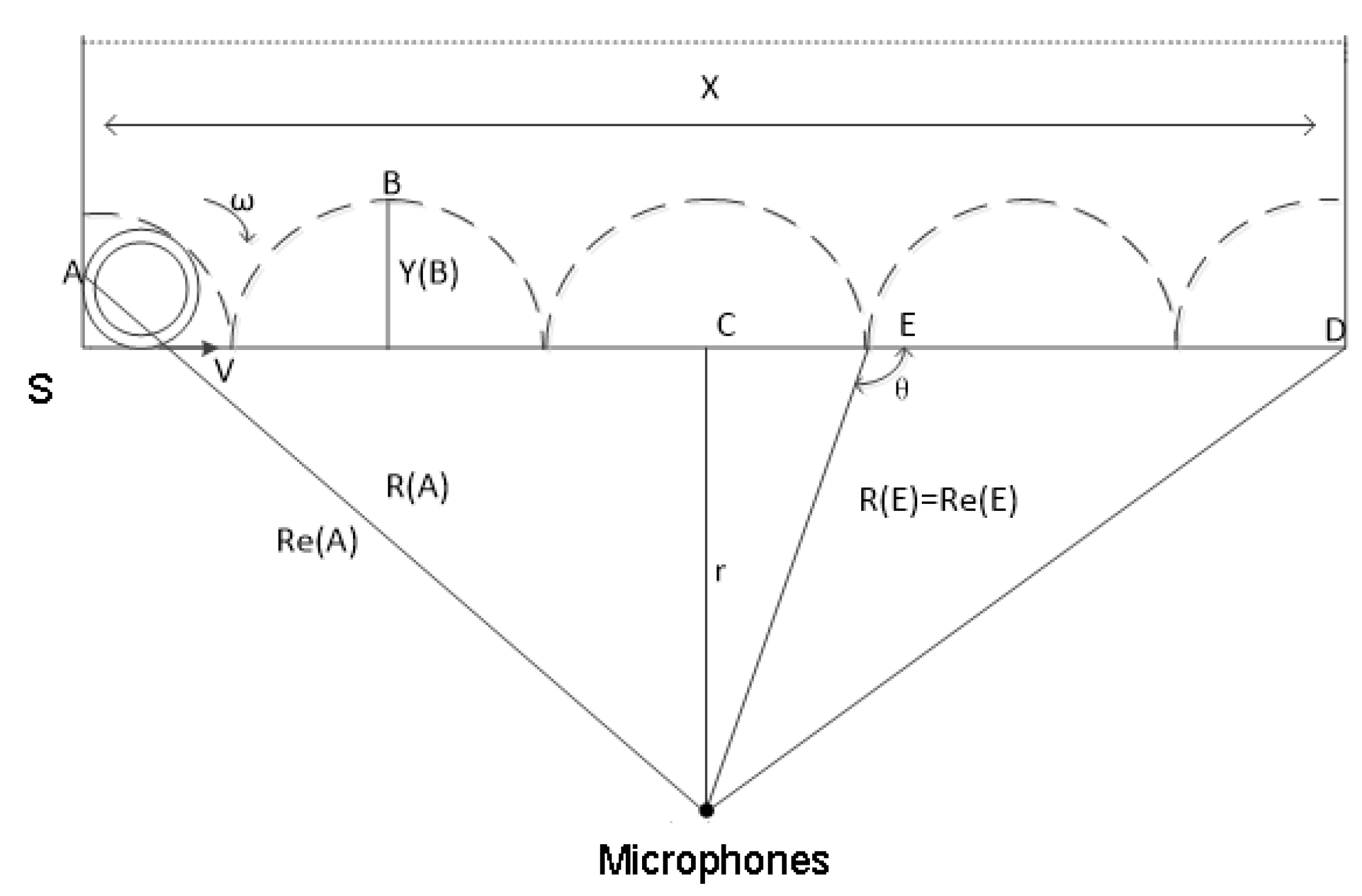
2.1. Rolling Bearing Failure Sound-Source Motion Model

When trackside acoustics are utilized for detection, the acquisition device is positioned at a fixed being installed on the train. The train maintains a constant and uniform speed, resulting in relative motion between the acquisition device and the bearing fault sound source. This relative motion causes Doppler distortion of the collected signal. The trackside acoustic system is illustrated in Figure 1, where 1 represents a magnetic sensor utilized for wheelset detection on passing trains. Auxiliary detection devices include 2, an infrared camera employed to inspect the underside of the car, and 3, a high-definition camera used for capturing train numbers. Additionally, 4 denotes a microphone employed for collecting fault signals from the wheelset bearing. Based on the positional relationship between the train wheel set and the acquisition device, a schematic diagram of the rail-edge acoustic detection device is established, as illustrated in Figure 2.

According to the physical model, a trackside acoustic detection test bench was constructed in the laboratory, and a bearing fault sound-source movement model was established. As illustrated in Figure 3, the bearing fault sound source undergoes a uniform linear motion from left to right, while simultaneously performing rotational motion along the vertical horizontal plane. The motion trajectory of the faulty sound source S is illustrated in the figure, where the horizontal distance of the motion path is X. The faulty bearing source moves with a uniform linear velocity v in the horizontal direction and rotates around the axis with an angular velocity ω in the vertical-horizontal direction. Using point A as the initial reference, the motion is executed along the trajectory illustrated in the diagram. When arriving at point B, take point B as the specific location of the fault sound source at a certain time, set the distance between the fault sound source and the acquisition device as Y(B), map the fault sound source to point E on the horizontal plane, and the distance from the fault sound source to the acquisition device as Re(E). In this case, the distance R(E) and Re(E) from the acquisition device to point E are equal. The angle between the horizontal motion trajectory and Re(E) is θ, the closest point of the acquisition device to the fault sound source is C, and the distance is r. When the fault sound source reaches point D, the distance from the fault sound source to the acquisition device is Re(D), and c is the propagation speed of sound in the air (M = v/c is Mach number). In view of the fact that the train speed is relatively much smaller than the sound propagation speed in the air, this analysis only focuses on the relevant problems when the faulty sound source moves at subsonic velocity, that is, M < 1 [27].

The fault sound source rotates around the bearing center, with the bearing center as the center of rotation. Based on the motion model of the bearing fault sound source, a plane rectangular coordinate system is established with the sound source s as the origin. In this case, let (x, y) represent the new coordinates of the fault sound source (0, 2R₁) after rotating a certain angle, where R₁ denotes the outer diameter of the faulty bearing. By applying relevant theoretical knowledge, we derive the geometric relationship between the fault sound source and acquisition device using the following formula:

$$x_1=v\cdot t$$

(1)

$$x=-R_1\cdot \sin \omega t$$

(2)

$$y=R_1+R_1\cdot \cos \omega t$$

(3)

$$v_x=R_1\cdot \omega \cdot \cos \omega t$$

(4)

$$R_e=\sqrt{r^2+{[(x_1+x)-(v+v_x)\cdot (i-1)\cdot t]}^2}$$

(5)

$$R_{11}=\sqrt{R_e^2+y^2}$$

(6)

2.2. Analysis of the Causes of Doppler Aberrations in Rolling Bearings

The derived equation for the geometric relationship obtained from the above analysis leads to the conclusion that the distance between the acquisition device and the bearing fault sound source exhibits a non-linear variation over time. The signal received by the microphone from the bearing fault sound source undergoes nonlinear changes. Consequently, the acquisition device also captures the bearing fault sound-source signal with non-linear variations. However, due to the equal time intervals at which the acquisition device collects the signal, a linear relationship is established during acquisition [28]. The sound source of the bearing fault undergoes a displacement in the vertical—horizontal plane during its propagation. Therefore, it is necessary to consider this displacement when determining the distance between the bearing fault sound source and the acquisition device. As a result, we express this distance as Formula (6). The acquisition device captures the bearing fault signal with a time delay phenomenon, which is represented by Equation (7), while Equation (8) illustrates the temporal sequence of receiving this signal, where c is the speed of sound in the air. R₁₁ is shown in Equation (6).

$$d{t}_i=\frac{R_{11}}{c}$$

(7)

$$T_i=(i-1)\cdot i+d{t}_i$$

(8)

The modeling process reveals a non-linear variation in the distance between the acquisition device and the bearing fault sound source, resulting in discrepancies in the sound pressure values of the acquired sound signals. Therefore, considering this as our theoretical foundation, we assume that the bearing fault sound source is a monopole point source, exhibiting uniform linear motion in the horizontal direction and rotational motion within its plane. Additionally, assuming an amplitude denoted by q representing the total mass flow rate emitted from the sound source s, we can express the distribution density of this point source as follows:

$$Q(\overrightarrow{r},t)=q(t)\delta (x-vt)\delta (y)\delta (z)$$

(9)

where q represents the total mass flow rate of the outgoing sound source S, x and y are obtained by Equation (2) and Equation (3), respectively, and the running speed of the faulty sound source of v bearing.

The fluctuation equation for the sound field can be expressed as follows [25]:

$${\nabla }^{2}P-\frac{1}{c}\frac{{\partial }^{2}P}{\partial t^2}=\frac{\partial }{\partial t}q(t)\delta (y)(z)$$

(10)

where p is the sound pressure and c is the speed of sound propagation in the air

The equation for the sound pressure of a bearing fault source received by the collecting device is derived based on the aforementioned equations and geometric relationships:

$$P=\frac{q^{\prime }(t-\frac{R}{c})}{4\pi R{(1-M\cos \theta )}^2}+\frac{q[t-\frac{R}{c}](\cos \theta -M)}{4\pi R{(1-M\cos \theta )}^2}$$

(11)

Equation (11) represents the variation in sound pressure of the bearing fault sound source during operation, where M denotes the Mach number, R stands for the outer diameter of the faulty bearing, and θ represents the angle between the horizontal motion trajectory and Re(E). This study focuses on investigating acoustic signals associated with wheel-bearing faults. Assuming that train speed is significantly lower than sound speed, it can be disregarded in this analysis as a factor affecting sound speed. Consequently, in the formula for sound pressure, the second term can be neglected relative to the first term without significantly impacting calculation results. For ease of computation, it is omitted here. By utilizing both the previous analysis on correlation between bearing fault sound source and acquisition device and considering fluctuations in sound pressure, we derive an expression for changes in sound pressure values of bearing fault sources during movement process, as shown by Equation (12):

$$P=\frac{\cos (\omega \cdot (t-\frac{R_{22}}{c}))}{4\pi R_{22}{(1-M\cdot \cos (u))}^2}$$

(12)

The sound pressure relationship of the bearing fault sound source can be derived from the aforementioned analysis. It is evident from the equation that the distance between the acquisition device and the bearing fault sound source exhibits non-linear variation, resulting in a corresponding non-linear change in sound pressure. Consequently, Doppler distortion primarily manifests as temporal and amplitude distortions in the acquired bearing fault signal. Therefore, it is necessary to correct for both time and amplitude aspects when addressing Doppler distortion.

2.3. Time Correction

According to the bearing motion model, the distance relationship and time sequence of the signal between the fault sound source and the acquisition device are obtained. The formula can be used to derive the time sequence of transmission from the fault sound source to the acquisition device. In practical detection processes, it is necessary for trains to continuously run. Consequently, during calculation of resampling time series, there will be constant changes in distance between the fault source and acquisition device. This dynamic aspect allows for more realistic and accurate time correction of distorted signals. Since signals are collected at equal time intervals while actual signal time series have unequal intervals, interpolation and resampling are required after collecting fault signals in order to obtain a more precise time series. The following equation presents the delayed time series and resampling time series corresponding to each point in operation:

$$d{t}_{i1}=\frac{R_{22}}{c}$$

(13)

$$T_{i1}=(i-1)\cdot t+\frac{R_{22}}{c}$$

(14)

The resampled time series is obtained by re-interpolating the faulty sound source’s time series T_i received by the acquisition device [29]. Interpolating and resampling a Doppler-distorted signal involves correcting the nonlinear variation in the acquired acoustic signal’s time series to a linear variation. In simpler terms, it means re-acquiring the acoustic signal using the same points and sampling frequency. Assuming that n and n + 1 are adjacent acoustic signals captured by the acquisition device, with coordinates (t_n, S_n) for point n and (t_n+1, S_n+1) for point n + 1, m represents an intermediate point between these two signal acquisition points. The schematic diagram can be seen in Figure 4.

The coordinates of point m are (t_m, S_m), where the sampling frequency and sampling interval of the bearing fault sound-source signal are known. The sampling interval is defined as 1/f, and a linear relationship is established between points n and n + 1 [12]. Furthermore, the following relationship holds true:

$$\frac{S_m-S_n}{t_m-t_n}=\frac{S_{n+1}-S_n}{t_{n+1}-t_n}$$

(15)

$$S_m=\frac{S_{n+1}-S_n}{t_{n+1}-t_n}(t_m-t_n)+S_n$$

(16)

The time series containing nonlinearity can be corrected through linear interpolation resampling, resulting in a new time series. At this stage, the signal has completed the process of interpolation resampling, indicating that the time correction of the acoustic signal has been accomplished.

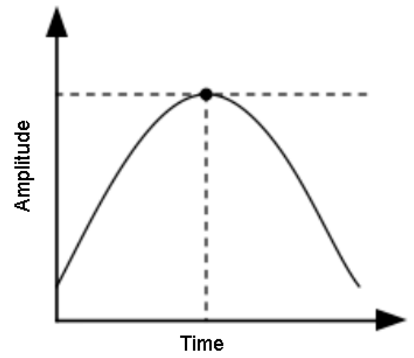
2.4. Magnitude Correction

The acoustic pressure of the signal received by the acquisition device varies with the changing location between the fault source and the acquisition device during train operation, resulting in amplitude distortion of the collected acoustic signal due to distance variation. In order to correct this Doppler-induced amplitude distortion in fault signals, a window function is created using the reference point closest to the acquisition device. The schematic is shown in Figure 5.

Equation (17) presents the derived sound pressure field of the bearing-failure sound source in the derivation process for the bearing motion model equation.

$$P=\frac{\cos [\omega \cdot (t-\frac{R_{22}}{c})]}{4\pi R_{22}{[1-M\cdot \cos (u)]}^2}$$

(17)

The sound pressure at the minimum distance between the bearing fault source and the acquisition device is utilized as the reference signal after amplitude correction of the fault signal. Subsequently, this sound pressure becomes a modulation function of the sound pressure generated by the relative motion between the bearing fault source and the acquisition device. The amplitude-corrected signal [14] can be expressed as shown in Equation (18). The acoustic signal obtained from Equation (18) undergoes theoretical corrections in both time and amplitude, resulting in an acoustic signal free from Doppler distortion.

$$S_f(t)=\frac{S_1}{A}$$

(18)

The distortion generated in time by the fault signal is corrected through a resampling algorithm. In terms of amplitude, the reference point closest to the acquisition device is utilized to create a window function, which compensates for the amplitude and restores its initial size. After both time and amplitude correction, the authentic fault sound-source signal is ultimately obtained.

3. Cyclic and Smooth Characteristics of Rolling Bearing Fault Signals

3.1. Smooth Second-Order Cycle

The vibration signal of rotating machinery, characterized by its periodic rotation, not only contains numerous random components but also exhibits prominent periodic components. The second-order statistical characteristics of the signal are non-smooth, indicating a cyclic smoothness in the signal. Consequently, conventional signal processing methods fail to analyze and identify it effectively. Recognizing the significance of periodic changes in signal statistics for bearing fault diagnosis, it is essential to employ a cyclic smoothing analysis method to extract crucial information for analysis [16].

The second-order cyclic statistics in the cyclic smooth analysis method provide a more accurate characterization of the cyclic smoothness of the signal. By analyzing these cyclic statistics, we can gain a comprehensive understanding of the characteristics and patterns of vibration fault signals, enabling us to make more precise diagnoses. Therefore, this study primarily employs the second-order cyclic smooth statistic [30], specifically utilizing the cyclic autocorrelation function and the cyclic spectral correlation density function, to conduct thorough cyclic smooth analysis.

3.2. Cyclic Smooth Model for Rolling Bearings

The cyclic smooth model of rolling bearings is established to account for the cyclic smooth characteristics. It is assumed that pitting failure in rolling bearings occurs after T cycles, where s(t) represents a specific shock oscillation and A_i denotes the amplitude of the ith shock. Considering the complexity of the working environment, which includes various disturbances from environmental noise, a zero-mean smooth and randomized environmental noise n(t) is introduced. Based on this information, the pitting fault model can be formulated as follows:

$$x(t)={\displaystyle {\sum }_{i=1}{A}_{I}s(t-iT)+n(t)}$$

(19)

The failure frequency of various components in rolling bearings is analyzed in conjunction with a pitting failure model.

The structure of the rolling bearing is illustrated in Figure 6, where D (mm) represents the raceway diameter, d (mm) denotes the rolling body diameter, and α indicates the bearing contact angle. Let N represent the number of rolling bodies, and N (r/min) denote the shaft speed.

The inherent frequency of the bearing when rotating is:

$$f_r=\frac{N}{60}$$

(20)

Bearing inner-ring failure, when the frequency of the rolling body passing a point on the inner ring (BPI) is:

$$BPI=\frac{1}{2}n(1+\frac{d}{D}\cos \alpha )f_r$$

(21)

Bearing outer-ring failure, when the frequency of the rolling body passing a point on the outer ring (BPO) is:

$$BPO=\frac{1}{2}n(1-\frac{d}{D}\cos \alpha )f_r$$

(22)

Bearing-rolling-element failure, when the frequency of rolling elements through the inner or outer raceway (BS) is:

$$BS=\frac{1}{2}\frac{D}{d}[1-{(\frac{d}{D})}^2{\cos }^2\alpha ]f_r$$

(23)

Bearing cage failure, when the rolling body of the common rotational frequency and cage speed frequency are consistent (FT) for:

$$FT=\frac{1}{2}(1-\frac{d}{D}\cos \alpha )f_r$$

(24)

The cyclic frequency characteristics of the cyclic smooth failure for each component of the bearing can be deduced by combining the specific features and theoretical knowledge of each component and the characteristic frequencies associated with them, as presented in

Table 1. Cycle frequency characteristics in the event of failure of individual rolling bearing components.

Fault Type	Rolling-Element Fault	Inner-Loop Fault	Outer-Ring Fault
Cycle frequency characteristic	$n{f}_{BS}\pm m{f}_{FT}$	$n{f}_{BPI}\pm m{f}_r$	$n{f}_{BPO}$

where$m,n\in Z$ denotes the characteristic frequency of the rolling body; f_FT denotes the rotational frequency; f_BPI and f_BPO denote the characteristic frequencies of the inner and outer rings, respectively; and f_r denotes the rotational speed.

.

4. Experimentation and Analysis

The fault diagnosis process, illustrated in Figure 7, is established based on the theoretical knowledge presented in the preceding two sections. Firstly, a Doppler distortion correction algorithm is employed to rectify the time and amplitude of the fault signal, ensuring its freedom from any Doppler distortion. Subsequently, cyclic smooth autocorrelation and cyclic smooth density spectrum analysis are applied to process the signal. Finally, fault diagnosis is conducted.

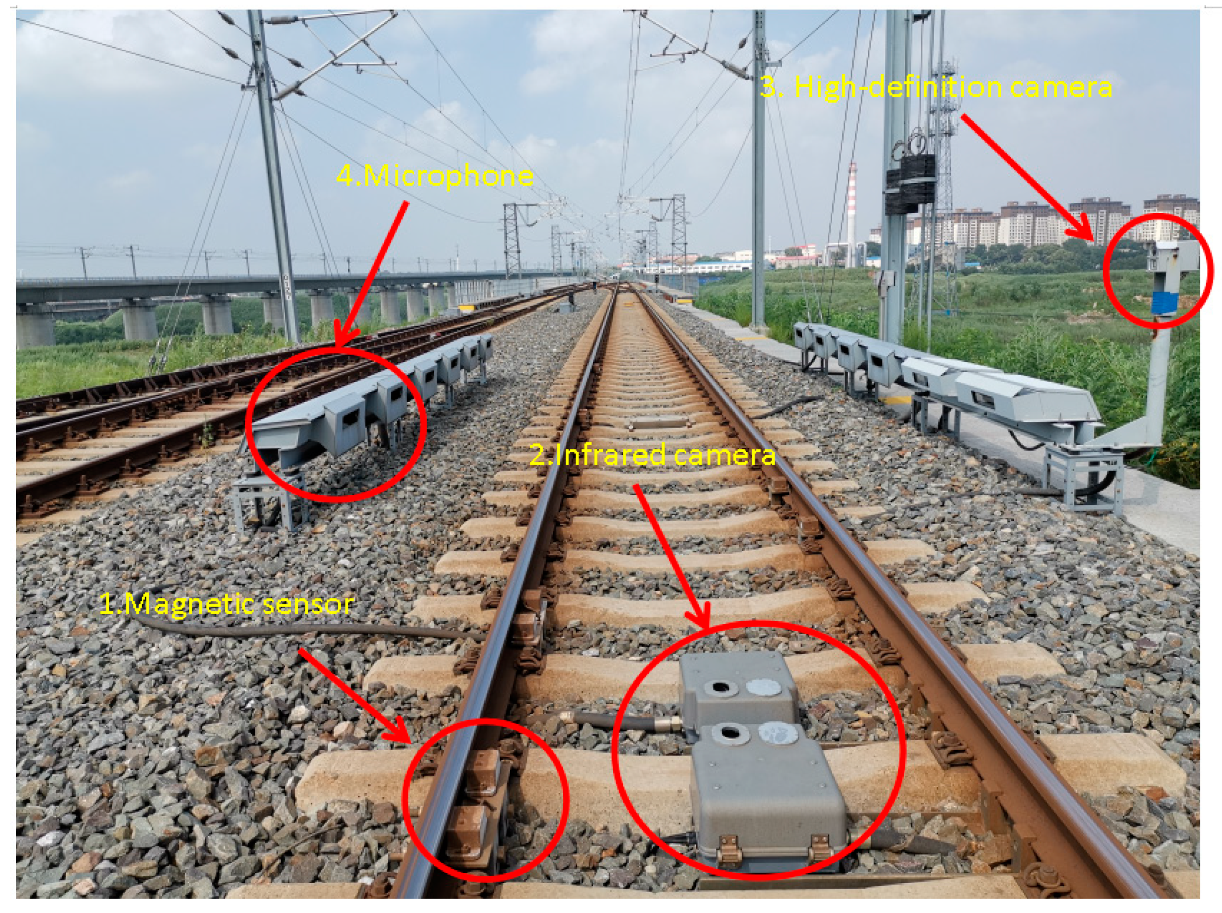
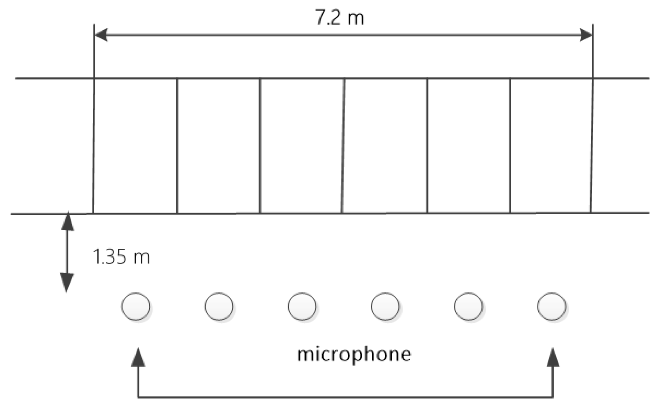
4.1. Trackside Acoustic Laboratory Bench

The trackside acoustic test bench, illustrated in Figure 8, comprises a servo motor, linear module, microphone, and acquisition card. This experimental setup emulates the motion of bearings in a trackside acoustic detection system and replicates the acoustic signals corresponding to various types of bearing faults [31]. It effectively simulates the actual operation of train bearings under simulated operating conditions while perceiving the bearing fault signals. In accordance with actual wheel operations, this experiment equates to a stable running length of 2 m within a 3-m long module. Additionally, the speed of the guideway experimental table can be adjusted between 0 and 3 m/s.

4.2. Rolling Bearing Experiments and Data Analysis

During the experiment, the bearing is loaded onto the slider and moves linearly in the horizontal direction. This means that the test bearing not only rotates perpendicular to the ground but also undergoes linear motion on a horizontally placed track. To accurately simulate the relationship between the bearing’s movement speed and its rotational speed in a train, it is necessary to set the horizontal speed of the slider to correspond with the vertical rotational speed of the bearing. In other words, the linear velocity of the test bearing during rotational motion is equivalent to that of the linear module slider. The calculation formula can be seen in Equations (25) and (26).

$$v_1=\frac{2\pi r{n}_1}{60}$$

(25)

$$n_2=\frac{60v_2}{s}$$

(26)

The equation above defines v₁ (m/s) as the equivalent horizontal linear speed of the test bearing and v₂ (m/s) as the speed of the linear module slider. It is important to note that v₁ and v₂ are numerically equal, i.e., v₁ = v₂. Additionally, n₁ (rpm) represents the speed of the test bearing, while n₂ (rpm) corresponds to the speed of the linear module AC motor. Furthermore, s (m) denotes the lead of the linear module, which refers to the displacement of the slider for one revolution of its drive motor. Please refer to your linear module manual for a specific value; in this case it is 0.165 m. Lastly, r (m) signifies the radius of the test bearing. The calculation results can be found in

Table 2. Calculation of rotational speed.

Test Bearing Speed n1 (rpm)	Slider Horizontal Speed v2 (m/s)	Slider Drive Motor Speed n2 (rpm)
150	0.4	145
300	0.8	291
600	1.6	582

.

The linear module slider requires a certain amount of time and distance to accelerate to the target speed as it moves horizontally in a straight line, and the same applies to the deceleration process. The effective length of the linear module is 3 m. To ensure that the slider does not collide with the edge block during movement, the first 0.5 m of the linear module is designated for placement and acceleration, while the second 0.5 m is used for deceleration. The middle 2 m represents the effective distance for actual signal acquisition. Positioned at a vertical distance of 1.35 m from the linear module, there is a microphone present in this experimental setup, as illustrated in Figure 9.

The trackside acoustic test bench is utilized to conduct bearing fault acquisition experiments, aiming to collect and analyze the acoustic signals for a wide range of experimental bearing faults. The known experimental bearing parameters are presented in

Table 3. Bearing parameters of bearing type N205.

Bearing Type	Inside Diameter (mm)	Pitch Diameter (mm)	Outside Diameter (mm)	Rolling Diameter (mm)	Number of Rolling Elements
N205	25	38.5	52	7.5	12

.

The test bearing can be manipulated to achieve different states by combining a damaged component with other intact components during the experiment, thus simulating the actual fault conditions of a real test bearing. The various types of faulty test bearings are illustrated in Figure 10.

Combined with the actual working conditions and the bearing motion model, the effect of data collection becomes more pronounced as the speed increases. Therefore, in order to verify the feasibility of the Doppler correction algorithm, a comparative analysis is conducted on the time domain waveform and power spectrum of the signal before and after correcting for outer-ring faults in bearings. As an example, a uniform speed of 1.6 m/s at 600 RPM is set for the bearing’s travel.

By comparing Figure 11 and Figure 12, it can be observed that the energy of the overall graph fault signal in Figure 12 is more concentrated, indicating a certain effectiveness of time domain correction and a slight increase in amplitude compared to Figure 11. This suggests that the algorithm processing improved the distortion to some extent by enhancing the amplitude. The comparison demonstrates that Doppler correction eliminates distortions in both time domain and amplitude to a certain degree. To further evaluate the corrective capability of the Doppler correction algorithm for distorted signals, power spectra of the initial signal and corrected signal for outer-circle faults are generated and compared, enabling clear visualization of changes. The power spectra for these signals are presented in Figure 13 and Figure 14.

By comparing the power spectrum of the initial signal in Figure 13 with that of the corrected signal in Figure 14, it can be observed that the overall image of the corrected signal exhibits a larger magnitude than the overall SNR (signal to noise ratio) of the initial signal, and there is a higher concentration of energy in the fault signal. This indicates that time-domain correction has achieved a certain level of effectiveness. In terms of the power spectrum image for the initial signal, we observe a prominent amplitude concentration between 200 and 300 Hz, accompanied by sidebands around 100–200 and 400–700 Hz. However, in the power spectrum image for the corrected signal, there is a significant increase (almost 50%) in amplitude at 200–300 Hz along with an approximately 25% increase in sideband amplitudes around both 100–200 and 400–700 Hz. These results demonstrate effective amplitude correction and elimination of distortion. Furthermore, through comparison between time domain waveforms and power spectra for outer-ring fault signals, we can conclude that the Doppler correction algorithm is feasible and yields good correction effects.

The bearing fault signal, after undergoing Doppler correction, is subjected to cyclic smoothing analysis in order to validate the accuracy and reliability of the bearing fault diagnosis method based on cyclic smoothing analysis with Doppler aberration correction. The experimental verification is performed using the example of the cyclic smoothing analysis applied to the bearing outer-ring fault signal after Doppler aberration correction. The cyclic autocorrelation spectrum of the initial signal for an outer-ring fault can be seen in Figure 15.

According to the established cyclic stationary model of the bearing fault and the specific parameters of the experiment, the cyclic characteristic frequency of a fault in the outer ring of the bearing is calculated to be 49.06 Hz. Cyclic stationary analysis is conducted on the fault signal from the outer ring after Doppler distortion correction, resulting in the cyclic autocorrelation spectrum illustrated in Figure 16.

The comparison between Figure 15 and Figure 16 reveals that as the SNR shown in Figure 16 increases, the active components of the fault signal are amplified, resulting in signals with prominent components in the cyclic autocorrelation spectrum. However, during signal processing, it is challenging to clearly observe cyclic frequencies and frequency components at other locations due to small amplitudes. To accurately determine characteristic cycle frequencies, appropriate processing methods must be adopted. The cyclic autocorrelation density spectrum of the initial signal’s outer-ring fault is displayed in Figure 17. A cyclic density spectrum analysis was conducted on the density spectrum function indicated in Figure 16 to obtain the cyclic autocorrelation density spectrum shown in Figure 18.

The comparison between Figure 17 and Figure 18 reveals that the active component of the fault signal in Figure 18 undergoes amplification, resulting in a highly pronounced cyclic characteristic frequency component within the cyclic density spectrum. Additionally, there are several sidebands observed near this cyclic characteristic frequency. Notably, a cluster of characteristic frequency points with concentrated signal distribution is evident in the figure. To ascertain the relationship between other characteristic frequencies, an elaborate analysis is conducted at these densely distributed characteristic frequencies, leading to the acquisition of a detailed slice diagram, as illustrated in Figure 19 and Figure 20.

The detailed slice diagram reveals the main frequency components, with 98 Hz corresponding to twice the characteristic frequency of the outer ring. This validates that cyclostationary analysis accurately detects fault signals in the bearing’s outer ring and highlights its characteristic frequency. Furthermore, a comparison between Figure 19 and Figure 20 demonstrates that after correcting for the fault signal in the outer ring, there is a significant amplification of active components. This indicates the feasibility of analyzing bearing fault signals post-Doppler correction and verifies the accuracy of the bearing fault diagnosis method based on Doppler distortion correction. Additionally, there are sidebands present in the detailed slice plot; however, their amplitudes are relatively small compared to those at the characteristic frequency and can be disregarded.

The method can be deemed correct and effective for bearing failure diagnosis, as it combines the bearing failure model and utilizes cyclic smooth analysis with Doppler aberration correction.

4.3. Project Example Analysis

To validate the efficacy of the proposed approach, a pre-existing TADS device was chosen within a vehicle section. The acquisition schematic of this device is illustrated in Figure 21, featuring a linear array comprising six microphones evenly spaced at a distance of 1.35 m from the track. With an acquisition range of 7.2 m, it facilitates capturing acoustic signals emitted by train bearings during uniform speed operation for subsequent analysis and identification of bearing signal faults.

Test bearing parameters are shown in

Table 4. Bearing parameters of bearing type 353130B.

Bearing Type	Inside Diameter (mm)	Pitch Diameter (mm)	Outside Diameter (mm)	Rolling Diameter (mm)	Number of Rolling Elements
353130B	150	200	250	22	23

.

During the inspection of the TADS equipment, anomalies were detected in the bearings. Subsequently, the novel bearing fault detection method proposed in this paper, namely the Doppler distortion correction method based on cyclic smooth analysis, was employed to analyze and process the bearing signals. The acquired acoustic signals underwent Doppler distortion correction, and a comparison was made between the time domain maps before and after correction. (Refer to Figure 22 and Figure 23 for further evaluation).

The comparison between Figure 22 and Figure 23 reveals that the SNR shown in Figure 23 exhibits a noticeable improvement compared to that in Figure 22. Additionally, the energy of the active component of the fault signal is amplified and more concentrated in Figure 23, indicating effective time domain correction. Moreover, there is a nearly 50% increase in amplitude compared to Figure 22 after algorithm processing, suggesting a certain level of distortion correction. The comparison of time domain waveforms reveals that both time domain and amplitude distortions are partially corrected following Doppler correction. To further assess the Doppler correction algorithm’s ability to restore bearing fault signals and correct Doppler distortion signals, power spectra for both the initial signal and corrected signal for outer-ring faults are generated and compared (Figure 24 and Figure 25).

By comparing the power spectrum of the fault signal in Figure 24 with that of the corrected signal in Figure 25, it can be observed that the overall image of the corrected signal exhibits an increased SNR compared to the initial signal. Furthermore, the energy of the fault signal is enhanced and more concentrated, indicating a successful time domain correction and rectification of time distortion. In terms of the initial signal’s power spectrum image, there is a prominent concentration of amplitude between 20 and 60 Hz, accompanied by sidebands around 100–120 and 160–200 Hz. However, in the power spectrum image of the corrected signal, there is a significant increase in power for fault signals within 20–60 Hz range by approximately 125%. Additionally, there is also an approximate increase by 25% in sidebands around 100–120 and 160–200 Hz. These observations demonstrate effective amplitude correction and rectification. Consequently, it can be concluded that by applying the Doppler correction algorithm, bearing fault signals were restored to their true form. The comparison between time domain waveforms and power spectra before and after bearing fault signal correction further confirms both feasibility and effectiveness of the Doppler correction algorithm.

The bearing fault signals, which have been corrected for Doppler aberration, were subjected to cyclic smoothing analysis in order to determine the type of bearing fault and verify the accuracy and feasibility of the diagnostic method based on cyclic smoothing analysis with Doppler correction. The resulting signal, after correcting for Doppler distortion, was then analyzed using cyclic smoothing techniques and the corresponding autocorrelation spectrum is presented in Figure 26.

The cyclic autocorrelation spectrum in Figure 26 reveals the presence of signals with prominent components. However, during the signal processing procedure, it is challenging to clearly observe the cyclic frequencies and frequency components at other locations due to their small amplitudes. To enhance our understanding of the cyclic characteristic frequency, we perform a thorough analysis using cyclic density spectrum and obtain the corresponding cyclic autocorrelation density spectrum, as illustrated in Figure 27.

The circular density spectrum in Figure 27 exhibits a distinct eigenfrequency component with prominent sidebands near the circular eigenfrequencies. Additionally, a cluster of signal concentrated distribution of eigenfrequency points is evident in the figure. To establish the relationship among the remaining eigenfrequencies, a refinement analysis was conducted on this concentrated distribution and yielded a refinement slice diagram, as illustrated in Figure 28.

The refined slice diagram reveals that the dominant frequency component is 76 Hz, accompanied by some minor frequency bands. However, their amplitudes are insignificant and can be disregarded. By integrating the cyclic smooth model of bearing failure established in Section 2 with the bearing speed of 396 rpm obtained from the TADS system and specific parameters of the bearing, we calculated the cyclic characteristic frequencies for each component in case of failure. The corresponding data are presented in

Table 5. Frequency of cyclic failure characteristics of rolling bearings.

Fault Type	Rolling-Element Fault	Inner-Loop Fault	Outer-Ring Fault
Cycle frequency characteristic	23.1 Hz	177.4 Hz	15.2 Hz

.

Comparison of characteristic frequencies in Table 5 reveals that the dominant frequency component of 76 Hz on the refined slice diagram illustrated in Figure 28 was five times higher than the outer-ring failure frequency of 15.2 Hz, leading to the deduction that the bearing failure occurred at the outer-ring location. Subsequently, disassembly of the bearing was carried out, as illustrated in Figure 29.

It is evident from the bearing failure diagram that the bearing failure was caused by a scratch on the outer ring of the bearing, resulting in an abnormal bearing signal detected by the TADS equipment. This confirms the accuracy of our previous inference. Therefore, utilizing cyclic smoothing analysis can effectively determine the location of bearing failure by identifying its cyclic characteristic frequency (or multiples thereof). This demonstrates both feasibility and accuracy when applying cyclic smoothing analysis to Doppler-corrected bearing fault signals, thus validating the reliability of our diagnostic method based on cyclic smoothing analysis with Doppler distortion correction. Through analyzing and verifying experimental and engineering signals, this paper illustrates the practicality and effectiveness of our proposed Doppler aberration correction method based on cyclic smoothing analysis.

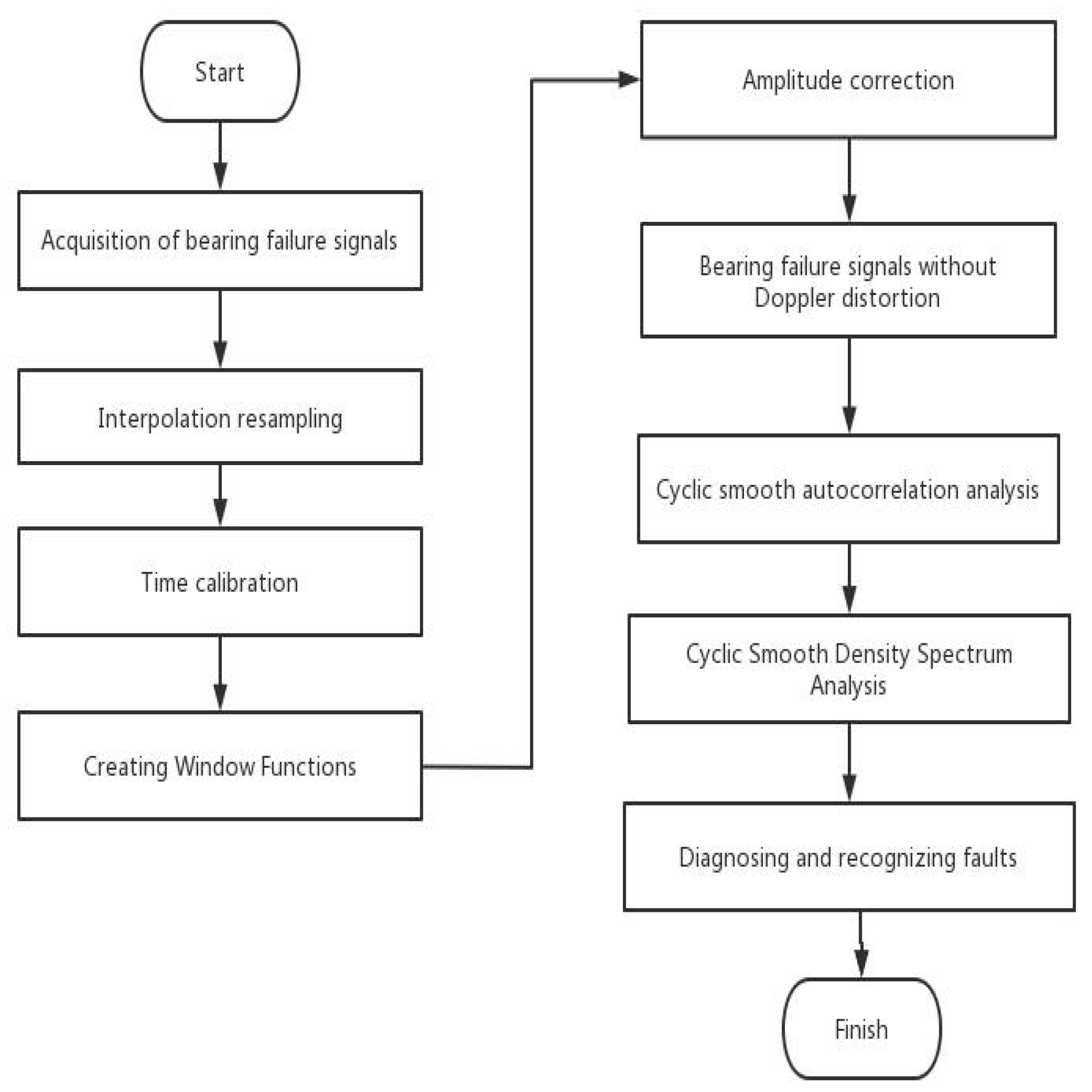
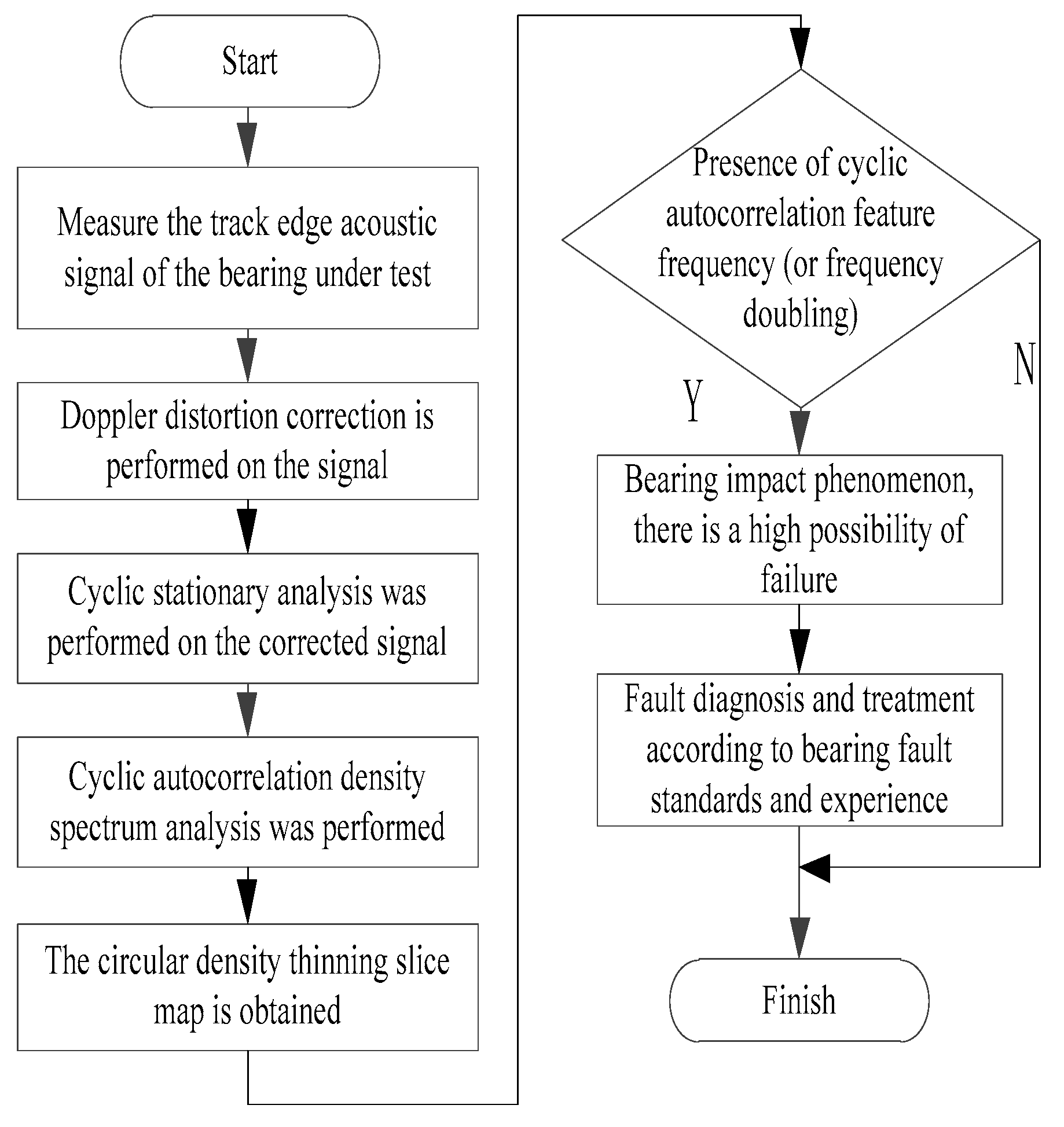
4.4. Steps in Bearing Fault Diagnosis

As follows, the steps for diagnosing rolling bearing faults with the Doppler aberration correction method based on cyclic smooth analysis are summarized by integrating the Doppler aberration correction algorithm, the cyclic smooth analysis method, and the rolling bearing model:

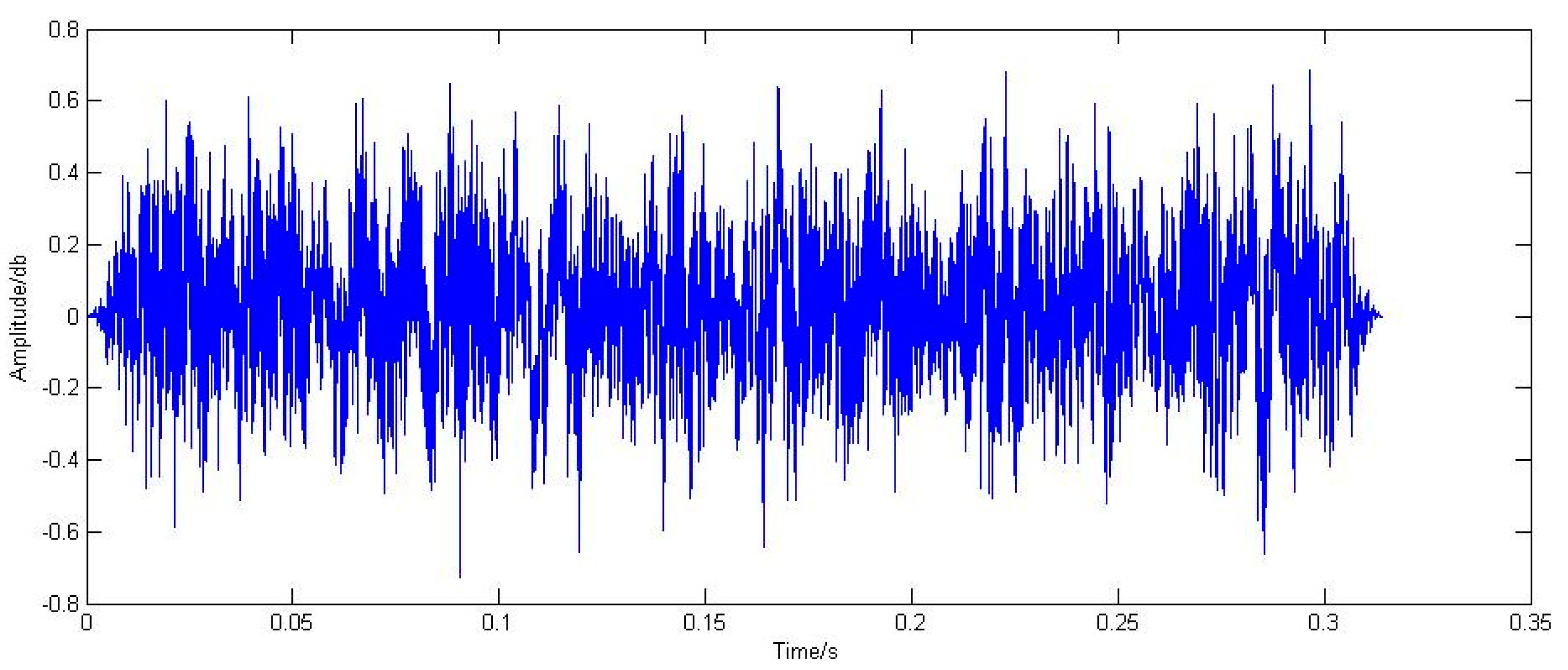
• The trackside acoustic signal of the bearing to be measured, primarily consisting of vibration and speed signals, is subject to measurement.
• The acoustic signals received trackside are corrected for Doppler distortion.
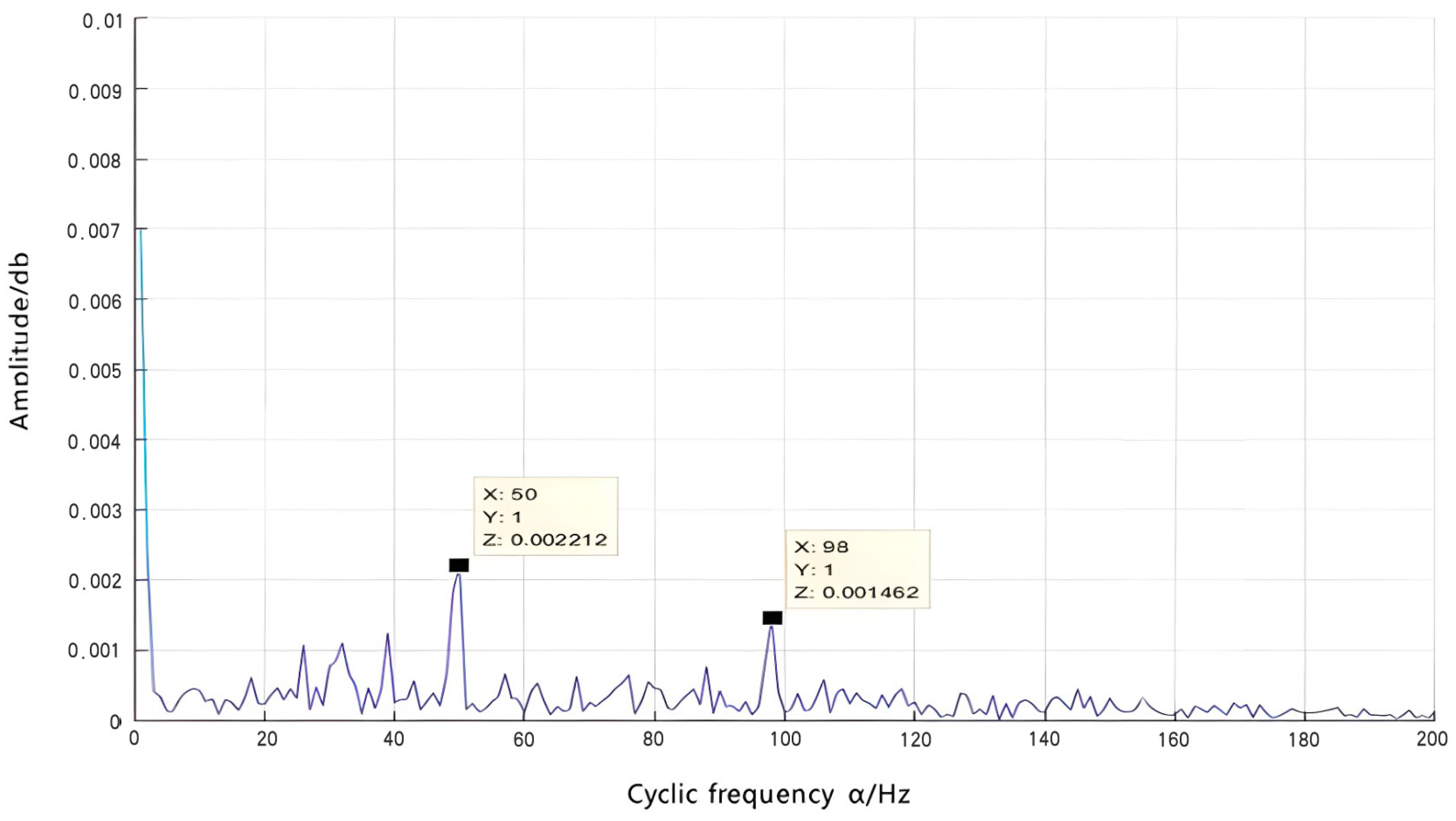
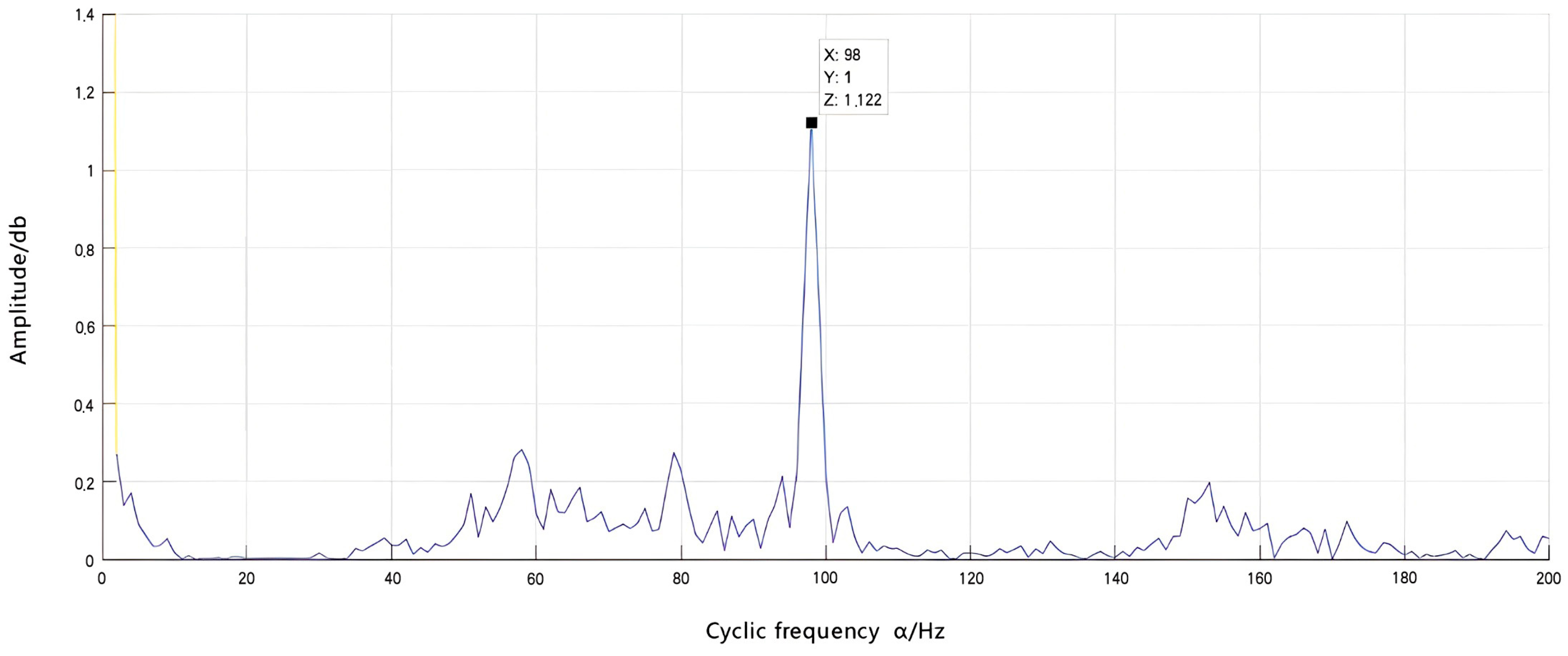
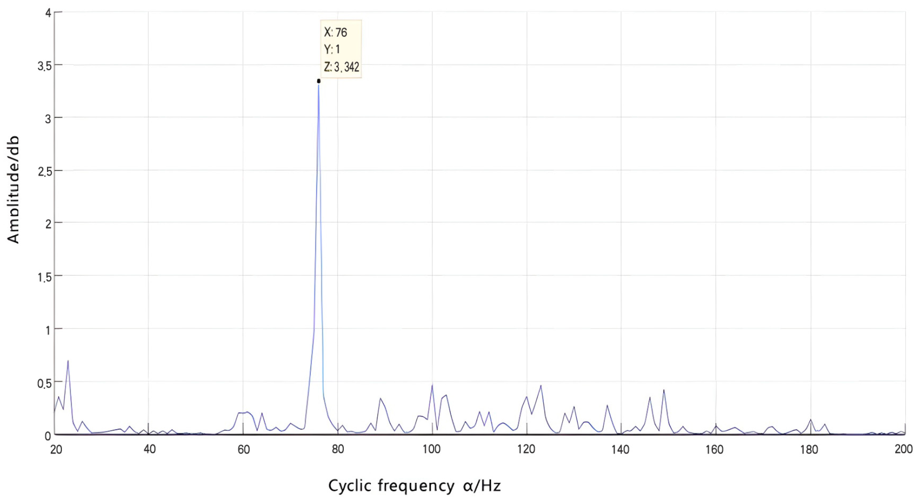
• The Doppler-corrected signal undergoes cyclic smoothing analysis. Firstly, a cyclic autocorrelation analysis is conducted to obtain a spectrum of cyclic autocorrelation. Secondly, the spectrum of cyclic autocorrelation density is examined to refine it into a slice of cyclic density refinement in order to determine the presence of a characteristic frequency or its multiple in the cyclic autocorrelation. If such frequency exists, it indicates the occurrence of shock phenomenon in the bearing at that time and suggests an impending failure.
• The faults are assessed based on predetermined criteria for evaluating bearing faults and practical experience to determine their impact on the component’s operation. Subsequently, appropriate handling procedures are implemented.

The sequence of diagnostic procedures is illustrated in Figure 30.

The proposed diagnostic procedure for faulty bearings is based on the Doppler distortion correction algorithm and cyclostationary analysis method investigated in this study. In comparison to the conventional diagnostic procedure, it is anticipated that the diagnostic accuracy will be enhanced by approximately 50%, leading to a reduction in error rate.

5. Summary

Based on the theory of Doppler correction and cyclostationary analysis, this paper presents a novel method for bearing fault diagnosis, namely the Doppler distortion correction method based on cyclostationary analysis. This method combines the characteristics of bearing fault signals, the Doppler correction algorithm, and the advantages of cyclostationary methods. Acoustic signals generated by bearing experiments were collected using a trackside acoustic experiment and processed using a Doppler distortion correction algorithm composed of interpolation resampling and numerical correction with window functions. The corrected signal was then analyzed using cyclic stationary analysis to compare and verify its time domain diagram, power spectrum diagram, and a cyclic stationary thinning slice diagram in order to demonstrate the feasibility of the method. To validate its applicability under practical conditions, existing TADS equipment from a car depot was used to collect bearing signals for further analysis and verification. This study explains both the applicability and effectiveness of this approach in real-world scenarios while also providing a fault diagnosis flow set for the Doppler distortion correction method based on cyclostationary analysis.

References

1. Sun, Y. Research on Key Technology of Rolling Bearing Fault Detection. Master’s Thesis, Harbin Engineering University of China, Harbin, China, 2019. [Google Scholar]
2. Ouyang, K. Research on Circular Array Short-Time Technique for Train Bearing Wayside Acoustic Signal Separation and Distortion Correction. Ph.D. Thesis, University of Science and Technology of China, Hefei, China, 2018. [Google Scholar]
3. Xia, J.; Liang, G. Trackside acoustic detector system(TADS) for rolling bearing of train. Harbin Bear. 2005, 6, 3–4. [Google Scholar]
4. Barke, D. Structural Health Monitoring in the Railway Industry: A Review. Struct. Health Monit. 2005, 4, 81–93. [Google Scholar] [CrossRef]
5. Choe, H.; Wan, Y.; Chan, A. Neural pattern identification of railroad wheel-bearing faults from audible acoustic signals: Comparison of FFT, CWT, and DWT features. Tex. A&M Univ. 1997, 30, 480–496. [Google Scholar]
6. Sneed, W.H.; Smith, R.L. On-board real-time railroad bearing defect detection and monitoring. In Proceedings of the 1998 ASME/IEEE Joint Railroad Conference, Philadelphia, PA, USA, 15–16 April 1998; pp. 149–153. [Google Scholar]
7. Southern, C.; Rennison, D.; Kopke, U. RailBAM: An advanced bearing acoustic monitor: Initial operational performance results. Core New Horiz. Rail 2004, 23, 01–07. [Google Scholar]
8. Snell, O.D.; Nairne, I. Acoustic bearing monitoring, the future RCM 2008. In Proceedings of the 4th IET International Conference on Railway Condition Monitoring, Derby, UK, 17–20 June 2008; pp. 32–47. [Google Scholar]
9. Zhang, S. Research on Time-Varying Array Analysis of Fault Spectrum Identification in Trackside Acoustic Diagnosis of Train Bearing. Ph.D. Thesis, University of Science and Technology of China, Hefei, China, 2017. [Google Scholar]
10. Zhang, A.; Hu, F.; Shen, C. Doppler distortion removal based on energy centrobaric method for wayside fault diagnosis of train bearings by acoustic signals. Vib. Shock 2014, 33, 17–19. [Google Scholar]
11. Liu, F.; Hou, C.; Zhai, T. An adaptive correction method for Doppler distorted signal of moving sound source. J. Acoust. 2022, 47, 820–831. [Google Scholar]
12. Zhang, H.; Lu, S.; He, Q. Fake time-frequency analysis of acoustic signals with Doppler distortion and its correction. Vib. Shock 2016, 35, 14–20. [Google Scholar]
13. Li, Q. Application Research on New Methods of Non-Stationary Signal Feature Extraction and Diagnosis. Techniques. Master’s Thesis, Tianjin University of China, Tianjin, China, 2005. [Google Scholar]
14. Bennett, W.R. Statistics of Regenerative Digital Transmission. Bell Syst. Tech. J. 1958, 37, 1501–1542. [Google Scholar] [CrossRef]
15. Gardner, W.A.; Franks, L. Characterization of cyclostationary random signal processes. IEEE Trans. Inf. Theory 1975, 21, 4–14. [Google Scholar] [CrossRef]
16. Gardner, W.A. Signal interception: A unifying theoretical framework for feature detection. IEEE Trans. Commun. 1988, 36, 897–906. [Google Scholar] [CrossRef]
17. Bonnardot, F.; Randall, R.B.; Guillet, F. Extractio of second-order cyclostationary sources—Application to vibration analysis. Mech. Syst. Signal Process. 2005, 9, 1230–1244. [Google Scholar] [CrossRef]
18. Leonardi, R.; Signoroni, A. Cyclostationary error analysis and filter properties in a 3D wavelet coding framework. Signal Process. Image Commun. 2006, 21, 653–675. [Google Scholar] [CrossRef]
19. Hanson, D.; Randall, R.B.; Antoni, J.; Thompson, D.J.; Waters, T.P.; Ford, R.A.J. Cyclostationarity and the cepstrum for operational modal analysis of mimo systems—Part I: Modal parameter identification. Mech. Syst. Signal Process. 2007, 21, 2441–2458. [Google Scholar] [CrossRef]
20. Boustany, R.; Antoni, J. Blind extraction of a cyclostationary signal using reduced-rank cyclic regression—A unifying approach. Mech. Syst. Signal Process. 2008, 22, 520–541. [Google Scholar] [CrossRef]
21. Bouaynaya, N.; Schonfeld, D. Nonstationary Analysis of Coding and Noncoding Regions in Nucleotide Sequences. IEEE J. Sel. Top. Signal Process. 2008, 2, 357–364. [Google Scholar] [CrossRef]
22. Urbanek, J.; Barszcz, T.; Antoni, J. Time–frequency approach to extraction of selected second-order cyclostationary vibration components for varying operational conditions. Measurement 2013, 46, 1454–1463. [Google Scholar] [CrossRef]
23. Lei, D. Research on the Non-Stationary Signal Based on Cyclic Stationary Feature. Master’s Thesis, University of Electronic Science and Technology of China, Chengdu, China, 2016. [Google Scholar]
24. Xu, W. Bearing Fault Diagnosis Based on Cyclostationary Analysis and Convolutional Neural Network. Master’s Thesis, Tianjin University of Technology and Education, Tianjin, China, 2022. [Google Scholar]
25. Luo, Z.; Xu, D.; Li, L. Bearing fault detection based on improved CYCBD method. J. Northeast. Univ. Nat. Sci. 2021, 42, 673–678. [Google Scholar]
26. Man, Y.; Guo, Y.; Wu, X. Robust rolling bearing fault feature extraction method based on cyclic spectrum analysis. Vib. Shock 2022, 41, 1–7. [Google Scholar]
27. Guo, X. Trackside Acoustic Signal Doppler Correction and Acoustic Detection Platform System Design. Master’s Thesis, Dalian Jiaotong University of China, Dalian, China, 2021. [Google Scholar]
28. Zhao, X. Study on fault diagnosis of rolling bearing based on angle-domain cyclostationary. Ph.D. Thesis, Dalian Jiaotong University, Dalian, China, 2017. [Google Scholar]
29. Liu, F. Research on Wayside Acoustical Fault Diagnosis for Train-Wheel Bearings when the Train Is Running at a Non-Uniform Velocity. Ph.D. Thesis, University of Science and Technology of China, Hefei, China, 2014. [Google Scholar]
30. Wu, Q.; Kong, F.; He, Q. Doppler shift correction for acoustic signals using resampling technique. Signal Process. 2012, 28, 1308–1313. [Google Scholar]
31. Han, Y. Design of Experimental Platform for Trackside Acoustic Detection Based on LabVIEW. Master’s Thesis, Dalian Jiaotong University of China, Dalian, China, 2022. [Google Scholar]
Figure 1. The trackside acoustic detection system.
Machines 11 00957 g001
Figure 2. Schematic diagram of the rai-edge acoustic detection device.
Machines 11 00957 g002
Figure 3. Sound-source motion model of bearing failure.
Machines 11 00957 g003
Figure 4. Resampling schematic.
Machines 11 00957 g004
Figure 5. Schematic diagram of amplitude correction.
Machines 11 00957 g005
Figure 6. Structure of the rolling bearing.
Machines 11 00957 g006
Figure 7. Fault diagnosis process based on cyclic smoothing.
Machines 11 00957 g007
Figure 8. Trackside acoustic testing experimental platform.
Machines 11 00957 g008
Figure 9. Experimental schematic.
Machines 11 00957 g009
Figure 10. (a) Test bearings outer-ring failure; (b) test bearing inner-ring fault; (c) test bearing rolling-element fault.
Machines 11 00957 g010
Figure 11. Outer-ring fault time domain waveform.
Machines 11 00957 g011
Figure 12. Corrected time domain waveform for the outer-ring.
Machines 11 00957 g012
Figure 13. Initial signal power spectrum of the outer-ring fault.
Machines 11 00957 g013
Figure 14. Power spectrum of the outer-ring fault correction signal.
Machines 11 00957 g014
Figure 15. Cyclic autocorrelation spectrum of the initial signal of the outer-ring fault.
Machines 11 00957 g015
Figure 16. Cyclic autocorrelation spectrum of outer-ring fault correction signal.
Machines 11 00957 g016
Figure 17. Cyclic autocorrelation density spectrum of the initial signal of the outer-ring fault.
Machines 11 00957 g017
Figure 18. Cyclic autocorrelation density spectrum of the outer-ring fault correction signal.
Machines 11 00957 g018
Figure 19. Slices of the cyclic density refinement of the outer-ring fault initial signal.
Machines 11 00957 g019
Figure 20. Slices of the cyclic density refinement of the outer-ring fault correction signal.
Machines 11 00957 g020
Figure 21. Schematic diagram of equipment acquisition.
Machines 11 00957 g021
Figure 22. Fault signal time-domain waveform.
Machines 11 00957 g022
Figure 23. Correction signal time-domain waveform.
Machines 11 00957 g023
Figure 24. Fault signal power spectrum.
Machines 11 00957 g024
Figure 25. Corrected signal power spectrum.
Machines 11 00957 g025
Figure 26. Cyclic autocorrelation spectrum.
Machines 11 00957 g026
Figure 27. Cyclic autocorrelation density spectrum.
Machines 11 00957 g027
Figure 28. Section of cyclic density refinement.
Machines 11 00957 g028
Figure 29. Bearing outer-ring failure diagram.
Machines 11 00957 g029
Figure 30. Fault diagnosis steps for rolling bearings.
Machines 11 00957 g030