Article

Hyperbolic-Secant-Function-Based Fast Sliding Mode Control for Pantograph Robots

Department of Telecommunications, Electrical, Robotics and Biomedical Engineering, Swinburne University of Technology, Hawthorn 3122, Australia
*
Author to whom correspondence should be addressed.
Machines 2023, 11(10), 941; https://doi.org/10.3390/machines11100941
Submission received: 28 August 2023 / Revised: 26 September 2023 / Accepted: 26 September 2023 / Published: 3 October 2023
(This article belongs to the Section Automation and Control Systems)

Abstract

:
Technological advancements in control systems are indispensable and require a robust controller with fast convergence in numerous sectors like robotics, space engineering, etc. A sliding mode controller (SMC) is a robust controller when subjected to nonlinearities, external disturbances, and uncertainties in system dynamics. However, SMC is prone to chattering, which can damage the plant in long term and results in low tracking accuracy. In this research paper, a novel hyperbolic secant function (HSF)-based SMC is proposed that achieves fast convergence, reduces chattering, and improves tracking performance. Stability analysis is conducted based on Lyapunov stability criteria. Comparative simulations and experiments on a pantograph robot (PR) show the effectiveness of the proposed algorithm.

1. Introduction

Robotic manipulators are considered a much-needed tool in the current era of industrial revolution. These manipulator are used for various purposes like cutting, mounting, transporting, and welding in numerous sectors where automatic precise machine operations are required. Pantograph robots are common for these type of industrial applications. A mechanical structure of four links connected in the form of a parallelogram is called a pantograph, where the motion of joint angles control the end-effector’s desired position, as shown in Figure 1. The end-effector’s accurate position control is required for a desired trajectory tracking task [1]. Forward, as well as inverse kinematics, along with the dynamics of a servo motor need to be derived for the accurate control of the end-effector of a pantograph robot (PR). Therefore, the end-effector position control of robotic manipulators has gained much attention from researchers [2].
Linear–quadratic regulators (LQRs) as well as proportional–integral–derivative (PID) controllers are commonly utilized by a combination of various intelligent control algorithms for these manipulators. These intelligent algorithms are specifically used for tuning the gains of LQR and PID [3,4], but the disadvantages of these basic algorithms lie in the key fact that these are unable to handle modeling errors or plant uncertainties. In [4], a genetic algorithm (GA) is combined with a PID controller to achieve the desired tracking, but it does not cope with the unmodeled system dynamics and parameters uncertainties. Moreover, the tuning of gains in PID controllers needs to be performed optimally. LQRs and PID controllers have been used for controlling the position of end-effectors of PRs, and particle swarm optimization (PSO) is also used for tuning purposes [5], but it lacks in tracking performance in the case of uncertainties. However, the introduction of optimization tools like GA, PSO, and Quantum PSO always enhances the complexity of a system, which eventually results in more overshoot with large steady-state error and even slow settling time with more iterations [5,6,7]. To address these issues and the disadvantages of the aforementioned algorithms, the SMC is considered to be a robust controller in such a scenario.
Sliding mode was designed in the era of the Soviet Union in the early 1950s [8]. In the case of model uncertainties, the robustness of SMC is a prominent feature [9]. SMC importance was neglected at that time because of chattering problems. However, the main benefits were considered, such as, for instance, the dynamic response of a plant in a closed-loop domain with a switching function makes the system robust against uncertainties. Therefore, researchers had a keen interest to investigate the pros and cons of SMCs. Currently, SMCs have been utilized as robust controllers in different fields pertaining to motion control, especially for precise tracking like in robotics, agriculture, automation and control manufacturing units, energy and mining industry, power electronics, and aerospace engineering [10].
The main reason behind the selection of SMCs is due to their robust properties against nonlinearities, external disturbances, and unknown model dynamics, as well as their reliability for multi-input multioutput (MIMO) systems. But, in spite of their many advantages, one of the prominent drawbacks of SMCs is chattering, which could damage the hardware during long runtimes. Another drawback of SMCs is slow convergence, as there is always a trade-off between faster convergence and chattering phenomena alongside better tracking performance, which eventually introduces large oscillations into systems. Chattering induces heat loss in electronic circuits, wear and tear of mechanical components, and results in low accuracy [11]. Although a fast SMC for a PR is proposed in [12], it is prone to chattering and not feasible for real-time applications. To address the chattering issues, a second-order SMC was developed, and then the higher-order SMC received much attention [13,14,15]. Then, disturbance-observer-based techniques were designed alongside SMCs with a feed-forward control in [16] to cope with chattering. Similarly, in [17], a disturbance-observer-based SMC was designed. Moreover, the boundary-layer strategy was also introduced in order to address discontinuity in the layer, but its drawback included that the ideal sliding mode was lost and eventually resulted in the cost of robustness [18]. To control the reaching process directly, as nonideal reaching in the reaching phase could also induce chattering, [19] proposed the reaching law strategy. Firstly, the constant reaching law was proposed, then the constant as well as proportional reaching law alongside the power reaching law were presented and extended to discrete-time systems [20,21]. Further modifications of these laws were also introduced [22,23,24]. Likewise, in [25], a continuous terminal SMC was proposed, but initial condition sensitivities led to large control inputs. Furthermore, in [26], an adaptive SMC based on barrier function was proposed for a linear motor. An integral-based fast terminal SMC was proposed in [27] for a permanent magnet synchronous motor.
An adaptive SMC based on proportional integral observer was proposed for a synchronous motor [28]. Recently, a pantograph control for high-speed trains based on rapid adaptation with deep meta-reinforcement learning was proposed. For transmitting electrical energy, a pantograph–catenary system is the vital component of the train, mounted at the top, which requires the robust control of a pantograph such that by the speed variation it optimally maintains contact and improves the current collection quality [29]. As discussed earlier, the introduction of intelligent optimization tools increases system complexity, needs more computational resources, and requires more iterations for optimal learning, which eventually makes the system slower. A robust control which requires less computational power, is simple in design, and feasible for real-time systems is much-needed. For nonlinear chaotic systems, an another adaptive fuzzy fractional control based on a supervised SMC is proposed to deal with uncertainties, but it is prone to slower convergence and overall lack in robustness for trajectory tracking [30].
Therefore, issues in regards to chattering, tracking performance, and faster convergence are still a huge challenge for researchers. Thus, this article contributes with an emphasis on the reduction in chattering, such that it should be feasible for real-time systems, along with faster convergence, stabilization, and improved tracking performance. Firstly, the novelty of the proposed algorithm includes a hyperbolic secant function, which is introduced in the power of a sliding surface such that it significantly reduces chattering. Secondly, a thorough stability analysis is carried out which guarantees the stability of the system. Lastly, the validation on hardware demonstrates the superiority of the proposed algorithm, and simulation studies verify the robustness of the proposed algorithm over the current existing state-of-the-art algorithms.
This article is organized such that Section 1 discuss the introduction. Section 2 consists of the mathematical modeling of the PR in which the servo motor transfer function is derived along with robot links kinematics, i.e., forward and inverse kinematics. In Section 3, the proposed control structure along with the stability analysis is explained briefly. Next, Section 4 includes the comparative simulation studies that are carried out in MATLAB/Simulink 2021a by considering a PR model. In Section 5, experimental results are outlined by considering three different cases for the PR with thorough discussion and implications, which show the effectiveness of the proposed algorithm. Finally, the conclusion is provided at the end.

2. Mathematical Modeling of the Pantograph Robot

The PR consists of two servo motors on which four links are attached, with each link being 5 inches in length. Two joints are actuated and three joints of the links are not actuated. As shown in Figure 1, two of the links are mounted on S R V 01 and S R V 02 on A and B points, respectively, and the control objective is to manipulate the end-effector position of the PR by controlling the cordinates of point E. In this section, mathematical modeling of the PR is carried out. Firstly, the transfer function and the state equation of the servo motor is given, followed by the inverse and forward kinematics of the PR links. Although the kinematics of the PR links are derived in [12], this paper presents much more details and thorough explanations.

2.1. Servo Motor SRV01

The servo motor consists of a linear or rotary actuator which is coupled with a motor and an encoder. It works in such a way that helps to accurately control the position or speed of a plant, and it is commonly used in robotics. The angular rate of the servo motor load shaft to input voltage ratio is represented by the following transfer function:
Ω m ( s ) U m ( s ) = K m T m s + 1 ,
where Ω m is the Laplace transform of ω m , which is the angular rate of the servo motor, and U m is the Laplace transform of control input u m , respectively. T m is the time constant, K m is the gain, and s is the Laplace operator. T m and K m are the nominal model parameters. The value of T m = 0.0254 (s) and K m = 1.53 (rad/sV). These nominal model parameters can be experimentally found by the bump test or by using frequency response. Equation (1) can be illustrated as follows:
Ω m ( s ) ( T m s + 1 ) = K m U m ( s ) ,
now, by the inverse Laplace transform, Equation (2) is simplified as follows:
ω ˙ m ( t ) T m + ω m ( t ) = K m u m ( t ) ,
where ω m ( t ) is the angular rate of the servo motor, i.e., ω m ( t ) = θ ˙ m ( t ) , substituting θ ˙ m ( t ) into (3) yields
θ ¨ m ( t ) = 1 T m θ ˙ m ( t ) + K m T m u m ( t ) .
The state vector is x ¯ = [ x 1 = θ m , x 2 = θ m ˙ ] T , and the state equation is expressed as follows:
x 1 ˙ ( t ) = x 2 ( t ) x ˙ 2 ( t ) = r ( x , t ) + g u m ( t ) + d ( t ) ,
In Equation (5), r ( x , t ) = 1 T m θ ˙ m , g = 1 T m K m , and d ( t ) are considered as external disturbances.
The state-space representation is given as follows,
x ˙ ( t ) = A x ( t ) + B u m ( t ) y ( t ) = C x ( t ) ,
where the state vector x ( t ) = θ m θ ˙ m , A = 0 1 0 1 T m , B = 0 K m 1 T m , and C = 1 0 .

2.2. Forward Kinematics

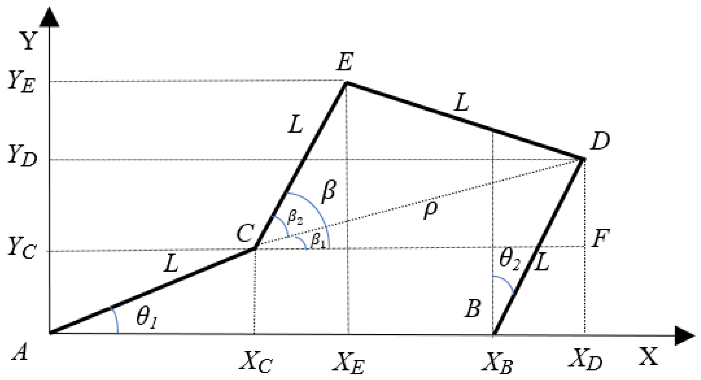
In forward kinematics, the end-effector coordinates along the X–Y axis need to be calculated, while θ 1 and θ 2 can be directly measured by the encoders of both servo motors, i.e., S R V 01 and S R V 02 , respectively, as shown in Figure 2.
Firstly, point C coordinates along the X–Y axis, i.e., X C and Y C are calculated and represented as follows:
X C = L cos θ 1 , cos θ 1 = X C L ,
Y C = L sin θ 1 , sin θ 1 = Y C L ,
where L = 5 (inch) represents the length of each link of the PR. Angular positions θ 1 and θ 2 along the axis of rotation are given in anticlockwise and clockwise, respectively. X B is known, i.e., X B = 2 L . Thus, point D components along the X–Y axis are written as follows:
X D = X B L cos 90 θ 2 = X B L sin θ 2 ,
Y D = L cos θ 2 ,
now, ρ needs to be calculated, which is the distance between point C and D. By applying the Pythagorean theorem on the triangle CDF, ρ is derived as follows:
ρ = Y D Y C 2 + X D X C 2 .
To find the end-effector, entitled coordinate E; the β angle shown in Figure 2 needs to be computed by the following equation:
β = β 2 + β 1 .
Next, by considering a bisector from point E on line C D such that it divides the length ρ into two equal lengths, i.e., ρ / 2 for each part, then β 2 and β 1 are calculated as follows:
cos β 2 = ρ 2 L , β 2 = arccos ρ 2 L ,
cos β 1 = X D X C ρ , β 1 = arccos X D X C ρ .
Substituting β 2 and β 1 from (13) and (14) into (12) yields β . Now, to calculate X E and Y E , β in terms of X E and Y E is written as follows:
cos β = X E X C L , β = arccos X E X C L .
sin β = Y E Y C L , β = arcsin X E X C L .
Based on (15) and (16), the PR end-effector coordinates along the X–Y axis, i.e., X E and Y E , are given as
X E = X C + L cos β .
Y E = L sin β + Y C .
Now, from (7) and (8), by substituting the values of X C and Y C into (17) and (18), the final expression of X E and Y E can be written as
X E = L cos θ 1 + L cos β . Y E = L sin β + L sin θ 1 .
In this section, X E and Y E are calculated as mentioned above in (19) when the positions of S R V 01 and S R V 02 are known, i.e., θ 1 and θ 2 , respectively.

2.3. Inverse Kinematics

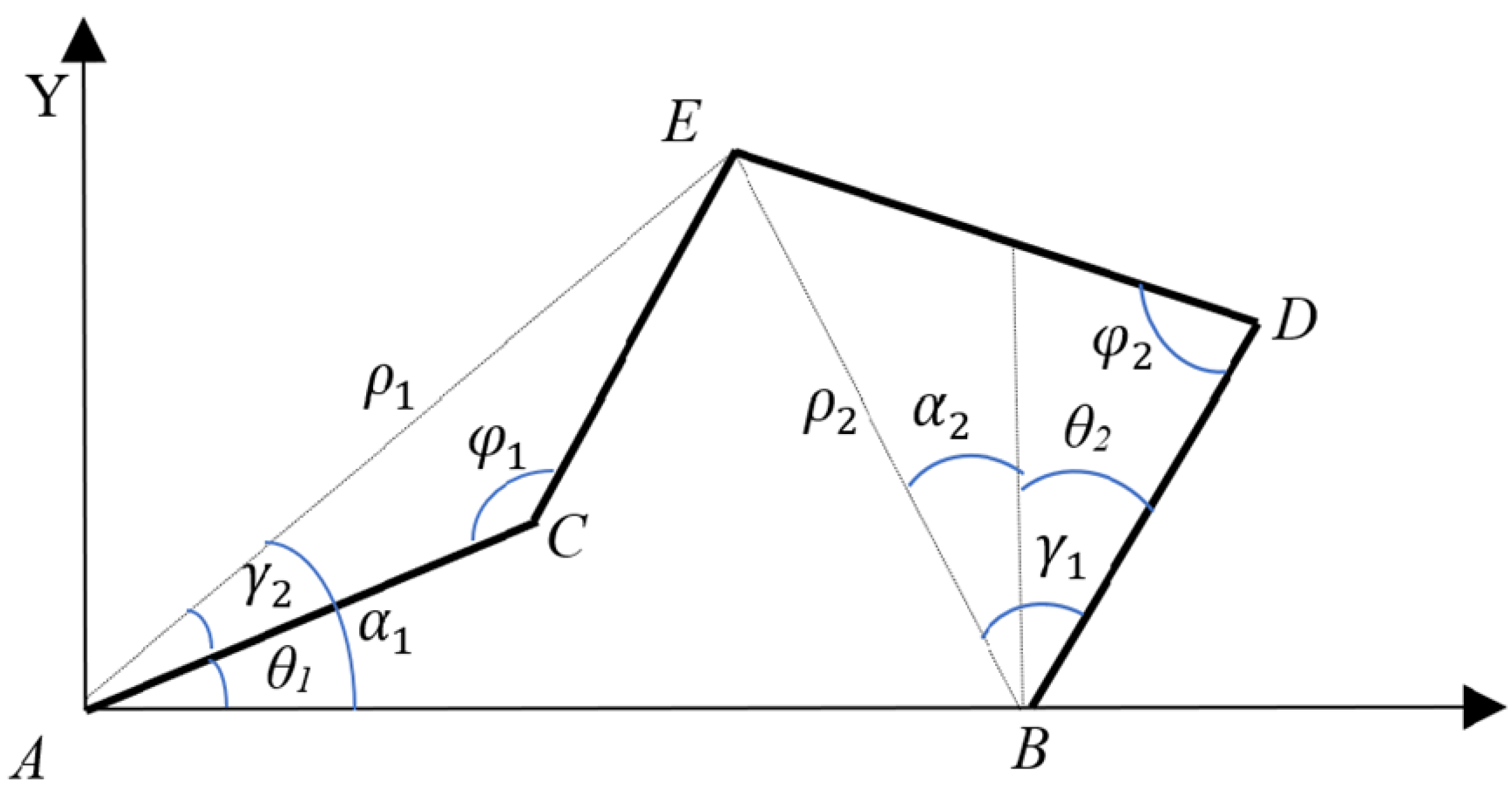
For the inverse kinematics, θ 1 and θ 2 need to be computed for the given end-effector E coordinates along the X–Y axis, i.e., X E and Y E , as shown in Figure 3.
At first, φ 1 and φ 2 , the angles across points C and D, need to be calculated by the following equations, where ρ 1 and ρ 2 are the distances between the A E and B E points, respectively, and L is the length of each link, i.e., L = 5 (inch).
φ 1 = arccos 1 ρ 1 2 2 L 2 ,
φ 2 = arccos 1 ρ 2 2 2 L 2 ,
where the values of ρ 1 and ρ 2 can be calculated as follows:
ρ 1 = X E 2 + Y E 2 ,
ρ 2 = B X E 2 + Y E 2 .
Now, the equations to derive the desired position angles of both servo motors of the PR, while the end-effector X–Y axis coordinates are known, i.e., X E and Y E , γ 1 , γ 2 , as shown in Figure 3, can be given as
γ 1 = π φ 2 2 ,
γ 2 = π φ 1 2 ,
where γ 1 and γ 2 are known as per (24) and (25), and α 1 and α 2 are calculated as follows:
α 1 = arctan Y E X E ,
α 2 = arctan B X E Y E .
The servo motors S R V 01 and S R V 02 position angles have the following expressions:
θ 1 = α 1 γ 2 .
θ 2 = α 2 γ 1 .
Now, substituting the values of γ 1 , γ 2 from (24), (25), α 1 , α 2 from (26), and (27) into (28) and (29), respectively, yields the final expression of the desired θ 1 and θ 2 in terms of X E and Y E , as per following equations:
θ 1 = arctan Y E X E π φ 1 2 . θ 2 = arctan B X E Y E π φ 2 2 .
In this section, the desired θ 1 and θ 2 are derived as per (30) for the given end-effector position along the X–Y axis, i.e., X E and Y E .

3. Design of the Proposed Control and Stability Analysis

In this section, firstly, the proposed control structure is explained, and then the proposed algorithm is derived, followed by the stability analysis.

3.1. The Proposed Control Structure of the PR

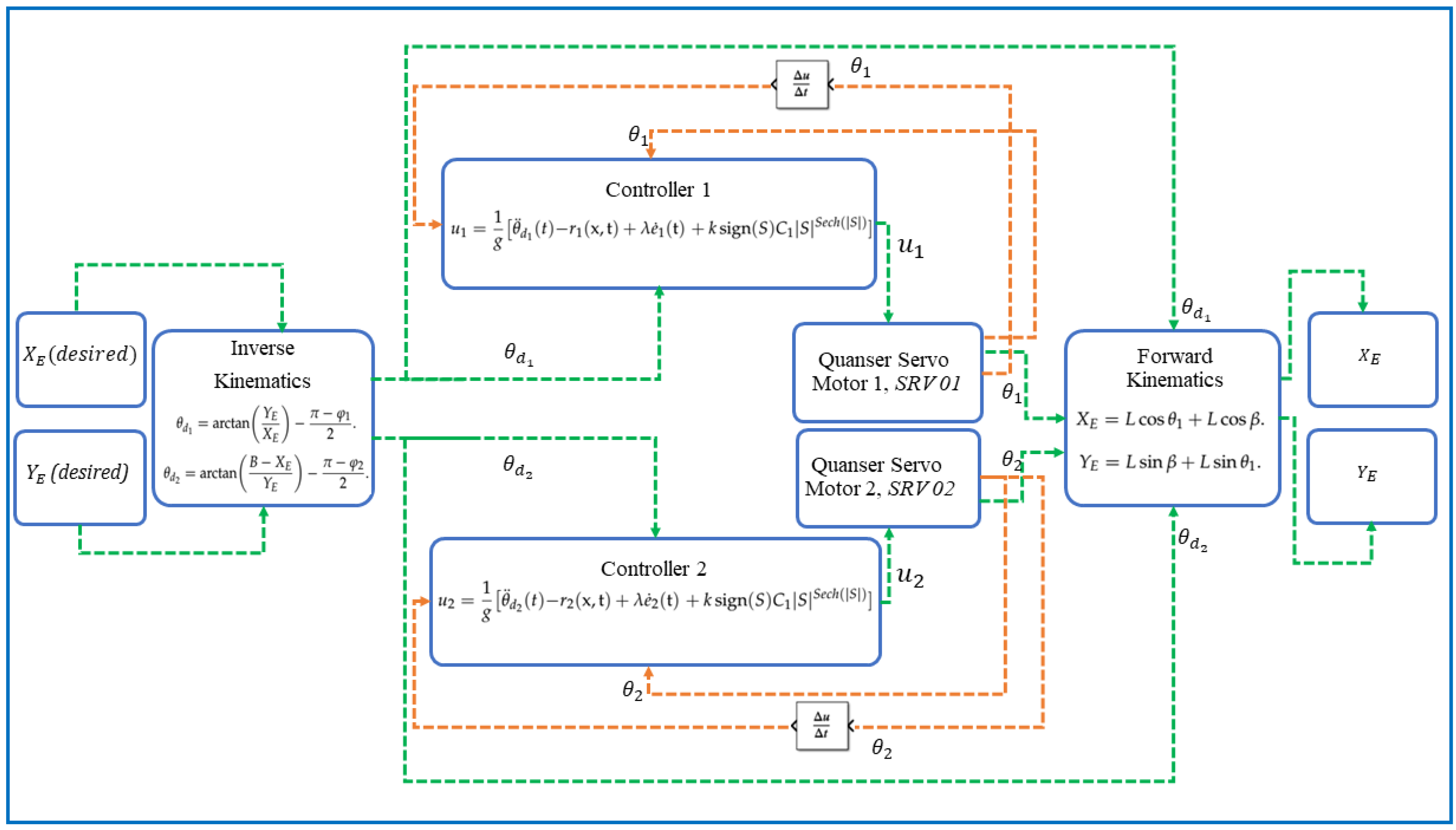
The proposed control structure of the PR is shown in the schematic block diagram in Figure 4.
At first, the desired position of the end-effector of the PR along the X–Y axis is given and, with the help of inverse kinematics as per (30), the desired θ d 1 and θ d 2 are calculated, which are required for the design of the proposed HSF-based SMC. As per Section 3.2, the proposed SMCs are designed, which can control the actual positions of both motors, i.e., θ 1 and θ 2 , by generating two control inputs u 1 and u 2 , respectively. Now, θ 1 and θ 2 are measured across the encoders of the servo motors S R V 01 and S R V 02 , and end-effector coordinates along the X–Y axis ( X E , Y E ) are derived accordingly as per the forward kinematics in Equation (19). In this way, the PR end-effector position is successfully controlled, as shown in Figure 4.
Simulations and hardware results verify the effectiveness of the proposed control, with less chattering, fast convergence, and better tracking performance.

3.2. The Proposed Hyperbolic-Secant-Function-Based SMC

In the proposed SMC, an appropriate switching function is first designed such that the system states can reach the sliding surface. Once, the states reach the sliding surface, a robust control law is necessary that enforces the states to slide across the designed sliding manifold. The following process outlines the steps to design the proposed control law.
First, the sliding surface can be designed as follows:
S = e ˙ ( t ) + λ e ( t ) , λ > 0
where the tracking error is represented as e ( t ) and can be chosen as follows:
e ( t ) = θ d ( t ) θ m ( t ) ,
e ˙ ( t ) = θ ˙ d ( t ) θ ˙ m ( t ) .
Taking the first derivative of (31) yields
S ˙ = e ¨ ( t ) + λ e ˙ ( t ) .
Substituting e ¨ ( t ) from (33) into (34) produces
S ˙ = θ ¨ d ( t ) θ ¨ m ( t ) + λ e ˙ ( t ) .
Based on (4), substituting θ ¨ m ( t ) into (35), we obtain
S ˙ = r ( x , t ) g u ( t ) d ( t ) + θ ¨ d ( t ) + λ e ˙ ( t ) .
Substituting S ˙ = 0 in (36), if d ( t ) = 0 , results in
u e q = 1 g r ( x , t ) + θ ¨ d ( t ) + λ e ˙ ( t ) .
A novel improved switching law is proposed as follows:
u s w = 1 g k sign ( S ) C 1 | S | S e c h ( | S | ) , u = 1 g r ( x , t ) + θ ¨ d ( t ) + λ e ˙ ( t ) + k sign ( S ) C 1 | S | S e c h ( | S | ) ] ,
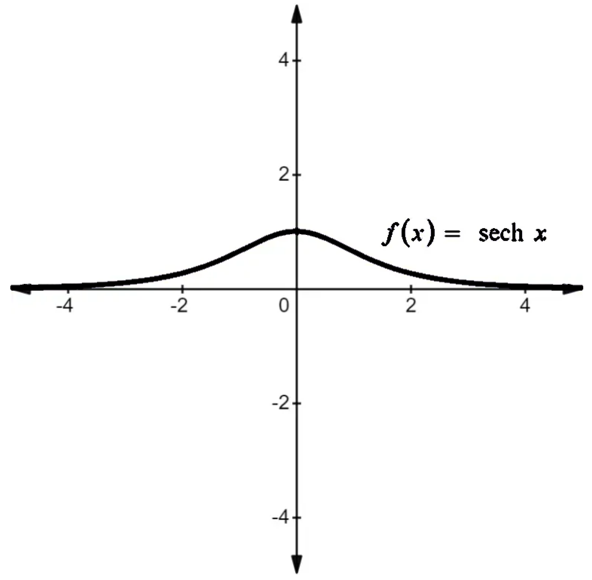
where λ > 0 , C 1 , k > 0 , r ( x , t ) = 1 T m θ ˙ m , g = 1 T m k m , and S e c h ( | S | ) ( 0 , 1 ] , as shown graphically in Figure 5.

3.3. Stability Analysis

The sliding surface as per Equation (31) is chosen as follows:
S = e ˙ ( t ) + λ e ( t ) . λ > 0
The first derivative of (39) yields
S ˙ = e ¨ ( t ) + λ e ˙ ( t ) .
Define a Lyapunov function as per [31],
V = 1 2 S 2 .
If the claim of the system’s energy decreasing with time is valid, then its derivative has to be strictly negative, i.e., S S ˙ < 0 . By substituting the value of S ˙ in the reachability condition, i.e., S S ˙ < 0 , we obtain
S S ˙ = S ( e ¨ ( t ) + λ e ˙ ( t ) ) .
Substituting e ¨ ( t ) from (33) into (42) gives
S S ˙ = S ( θ ¨ d ( t ) θ ¨ m ( t ) + λ e ˙ ( t ) ) .
Substituting θ ¨ m ( t ) from (4) into (43) yields
S S ˙ = S r ( x , t ) g u ( t ) d ( t ) + θ ¨ d ( t ) + λ e ˙ ( t ) ) .
Substituting r ( x , t ) and g from (5) into (44) results in
S S ˙ = S [ ( 1 T m θ ˙ m ) ( 1 T m k m ) u ( t ) d ( t ) + θ ¨ d ( t ) + λ e ˙ ( t ) ] .
Substituting u from (38) into (45), we obtain
S S ˙ = S [ ( 1 T m θ ˙ m ) ( 1 T m k m ) [ 1 g θ ¨ d ( t ) r ( x , t ) + λ e ˙ ( t ) + C 1 sign ( S ) k | S | S e c h ( | S | ) ] d ( t ) + θ ¨ d ( t ) + λ e ˙ ( t ) .
Substituting r ( x , t ) and g into (46) as d ( t ) = 0 produces
S S ˙ = S [ ( 1 T m θ ˙ m ) ( 1 T m k m ) 1 k m T m θ ¨ d ( t ) 1 T m θ ˙ m ) λ e ˙ ( t ) C 1 sign ( S ) k | S | S e c h ( | S | ) ] + θ ¨ d ( t ) + λ e ˙ ( t ) .
Further simplification of (47) yields
S S ˙ = S ( C 1 sign ( S ) k | S | S e c h ( | S | ) ) .
Case 1: In (48), if S > 0 ,
S S ˙ = S ( C 1 sign ( S ) k | S | S e c h ( | S | ) ) < 0 S S ˙ = S ( C 1 sign ( S ) k | S | S e c h ( | S | ) ) < 0 ; i f f C 1 , k > 0 , S e c h ( | S | ) ( 0 , 1 ]
Case 2: In (48), if S < 0 ,
S S ˙ = S ( C 1 sign ( S ) k | S | S e c h ( | S | ) ) < 0 S S ˙ = S ( C 1 sign ( S ) k | S | S e c h ( | S | ) ) < 0 ; i f f C 1 , k > 0 , S e c h ( | S | ) ( 0 , 1 ]
It is pertinent to mention here that if | s | 0 , | s | = 0 , | s | < 0 , or | s | > 0 , S e c h ( | S | ) is always bounded within the stable range, i.e., S e c h ( | S | ) ( 0 , 1 ] , as shown above in Figure 5, Hence, stability is guaranteed.

4. Comparative Simulation Analysis

This section outlines the simulation results carried out in MATLAB/Simulink (R2021a) on a PR model. The control structure is chosen as per Section 3.1. The desired reference signals given to the PR along the X–Y axis for tracking are X E d = sin ( π t ) + 0.5 sin ( π / 2 t ) + 5 and Y E d = sin ( π t ) 0.5 π + 0.5 sin ( π / 2 t 0.5 π ) + 5 , respectively. The comparison is performed with an SMC and a recent adaptive sliding mode control (ASMC) [28]. Firstly, comparative simulations with same control parameters are carried out, as per Section 4.1. For this purpose, the control parameters of the proposed SMC are selected as per Table 1. For the ASMC, gains are taken as c = 14 , k = 140 , and the rest of the parameters are n = 50 , λ = 0.20 . In Section 4.2, the optimal performance comparison of each controller is also conducted by individual tuning of each controller based on minimum chattering and better tracking performance.

4.1. Comparative Simulation with Same Parameters

Comparative simulation results with the same parameters are shown in Figure 6, Figure 7, Figure 8, Figure 9 and Figure 10.
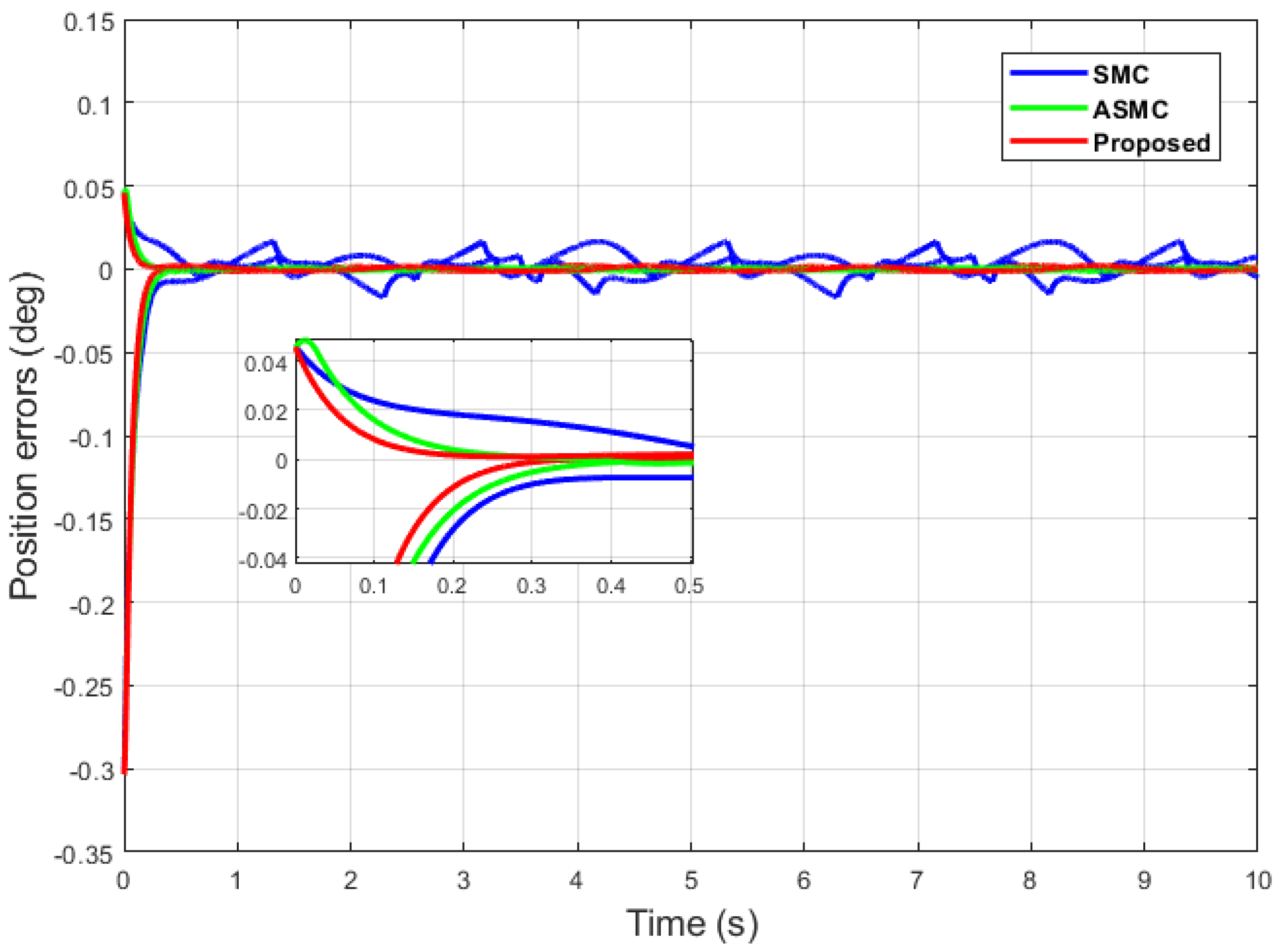
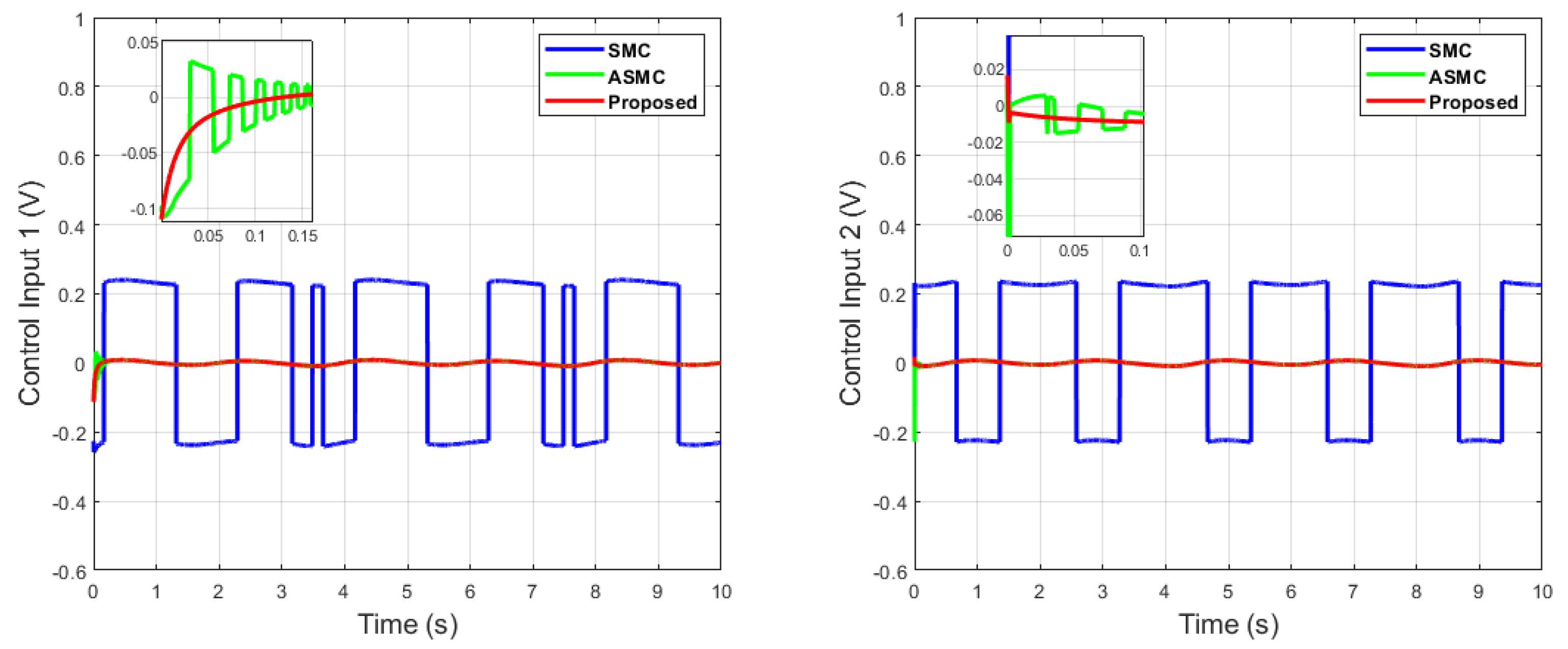
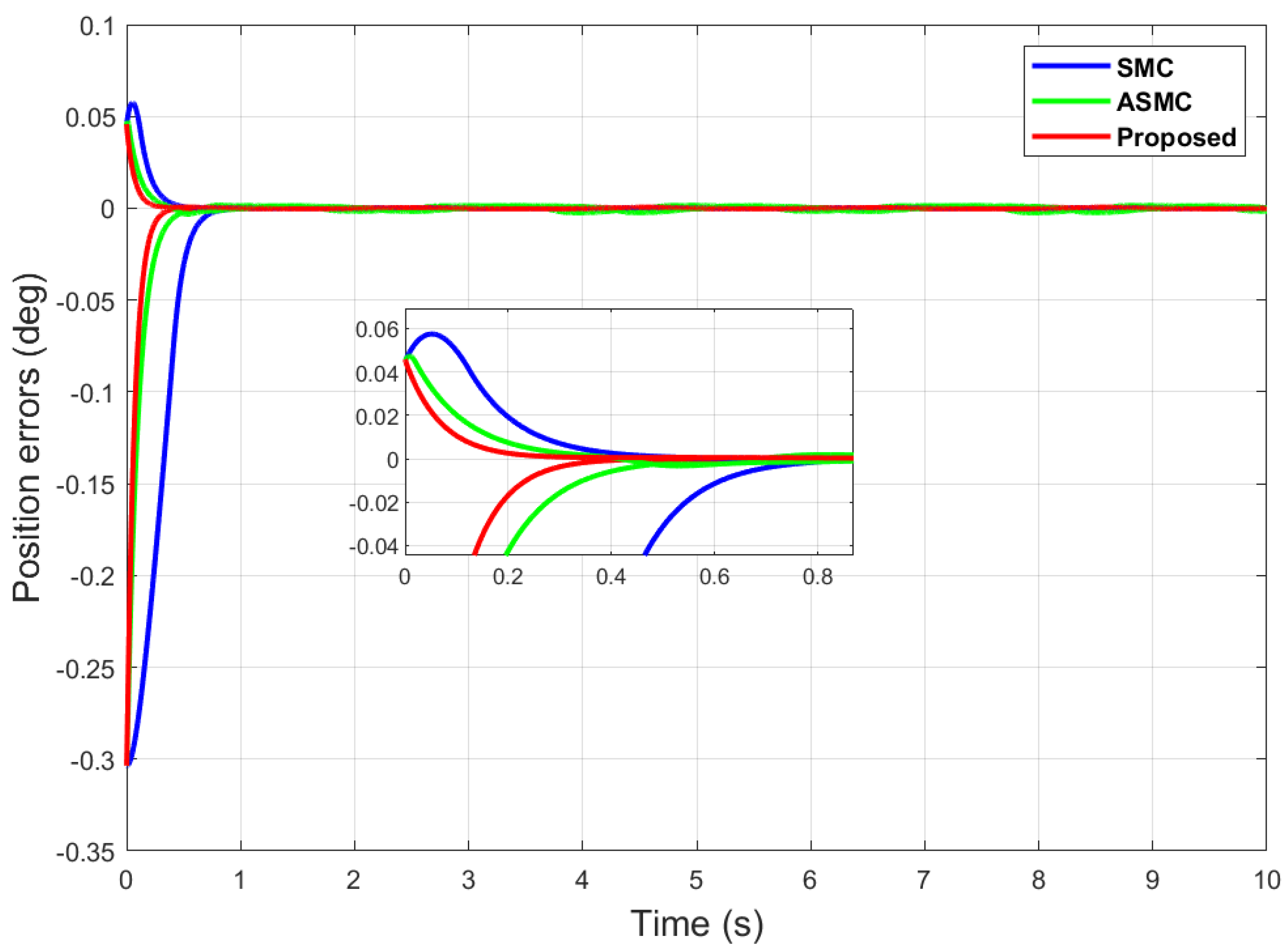
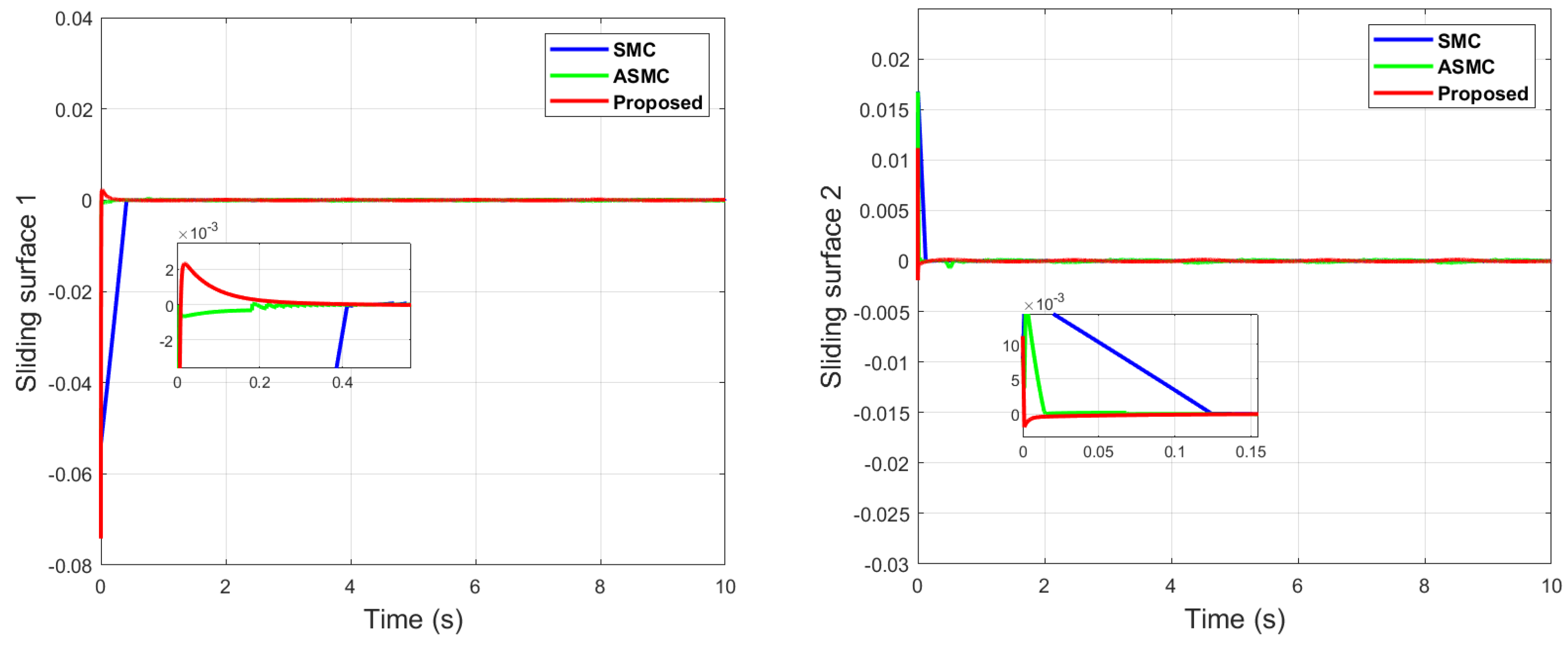
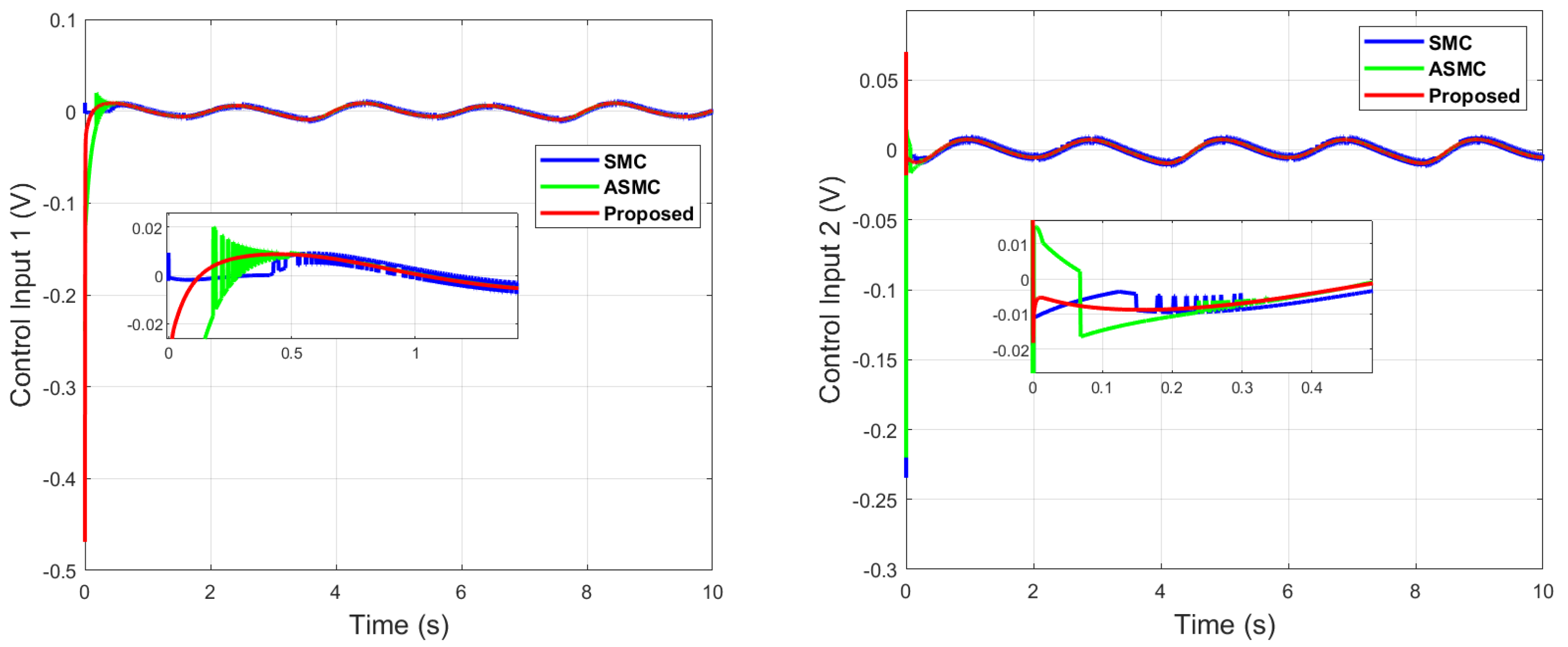
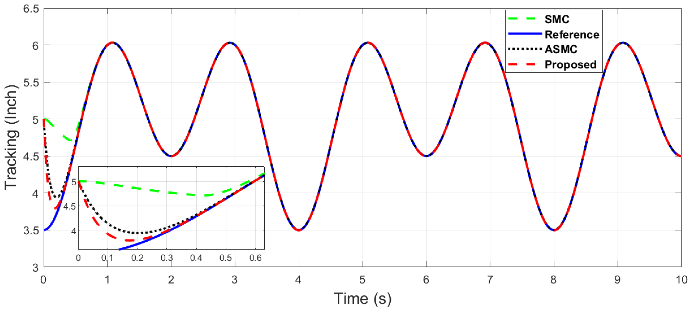
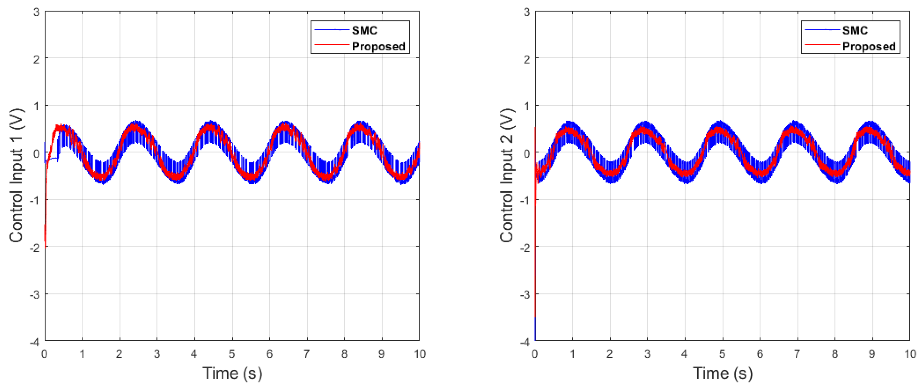
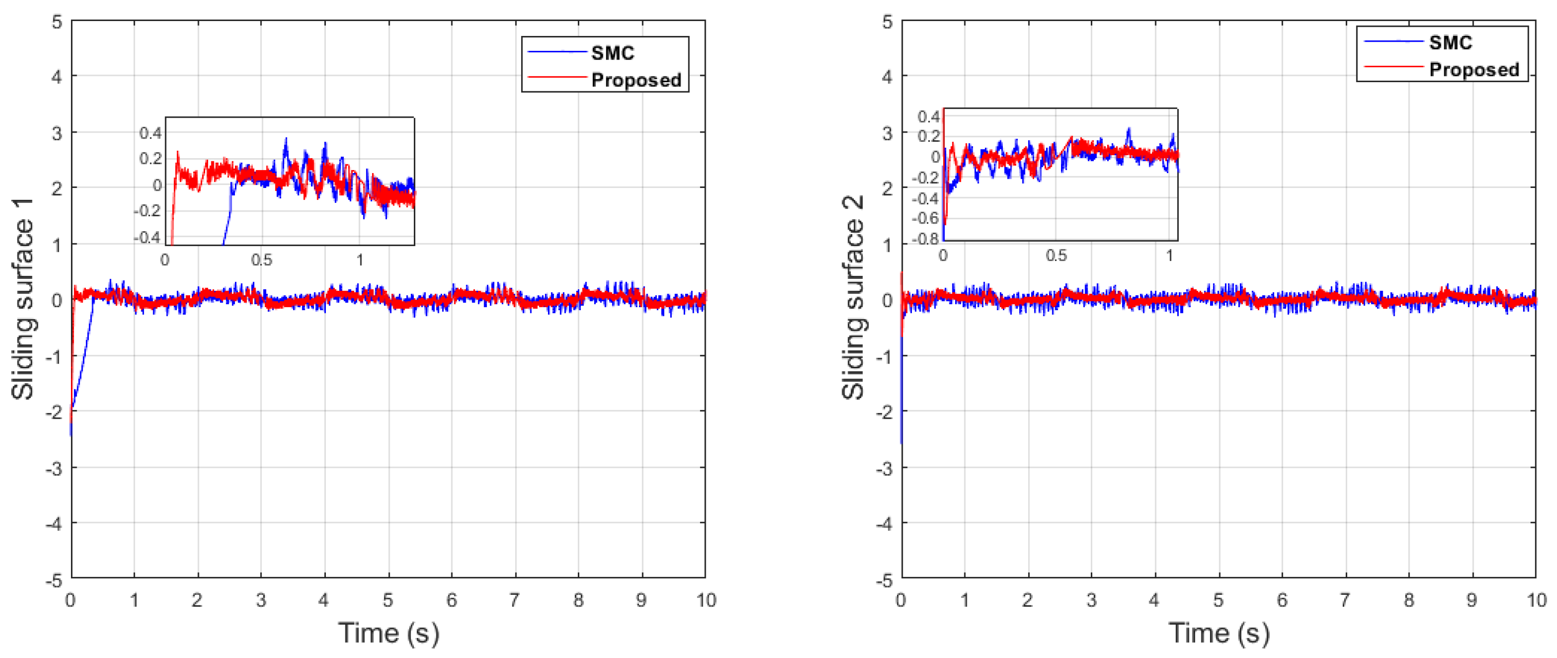
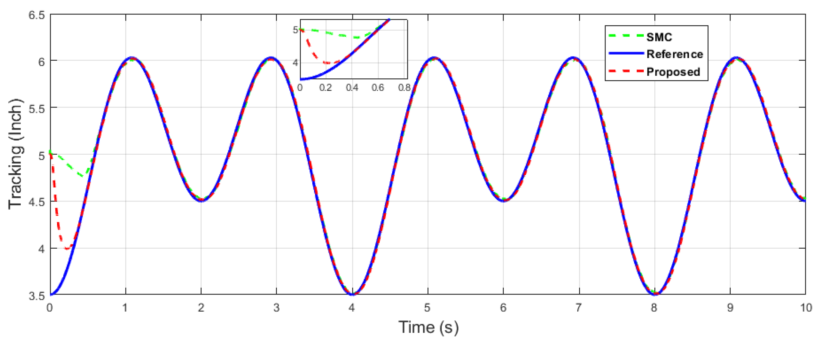
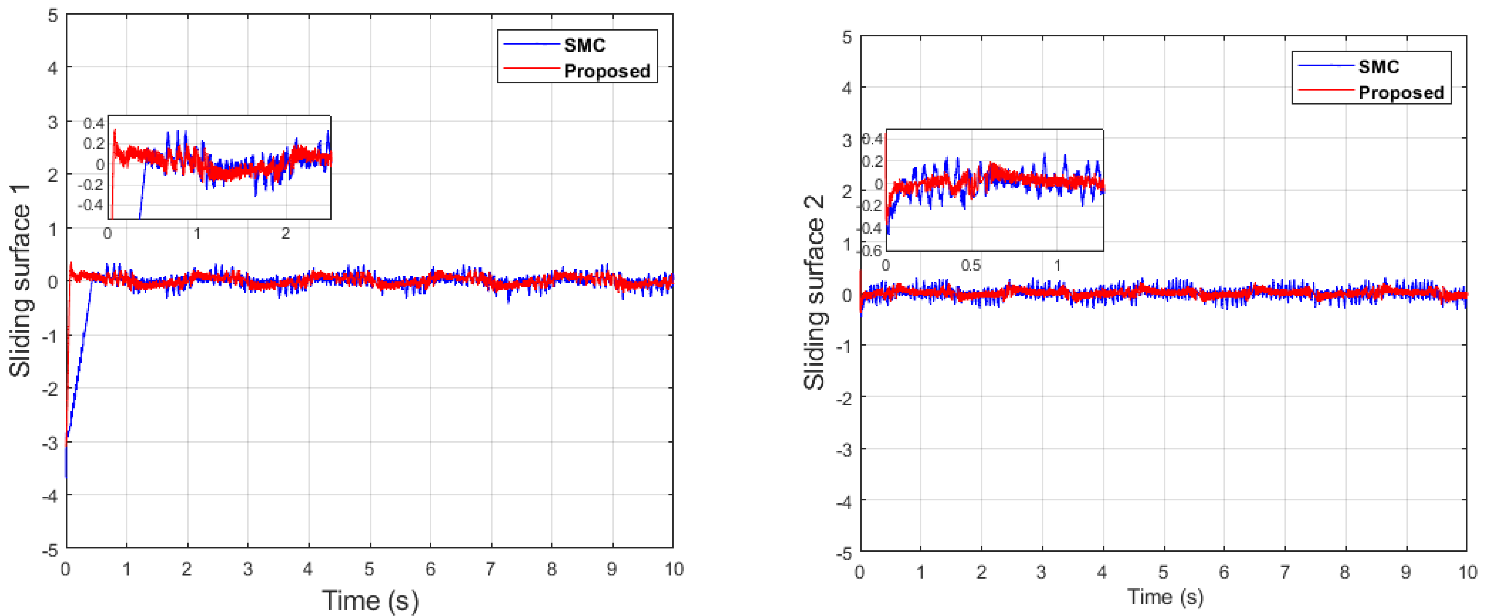
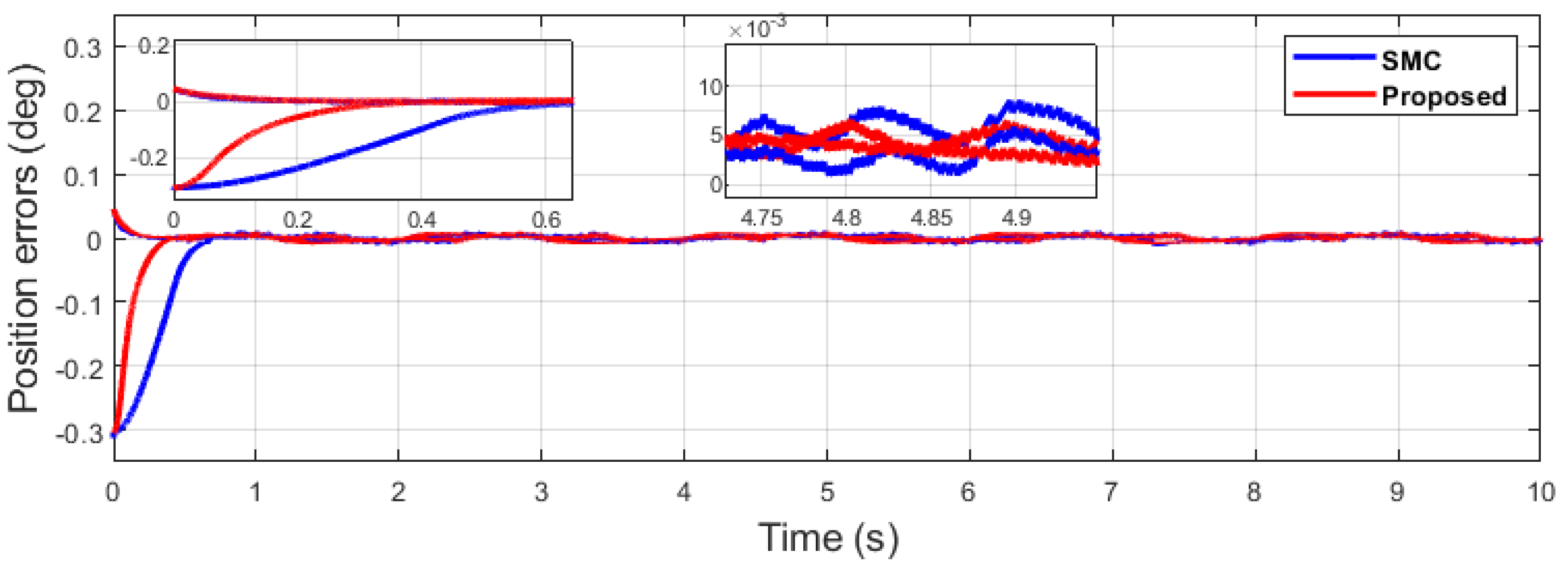
It can be seen from Figure 6 that in the case of dual-sine-wave tracking, the proposed algorithm outperforms the others with faster convergence, which can be seen in the zoomed section of Figure 6. In Figure 7 and Figure 8, the sliding surfaces comparison and control inputs comparison for dual-sine-wave tracking are conducted, respectively. However, the SMC input can be adjusted to a similar bandwidth for fair comparison in simulations, which further deteriorates its performance.
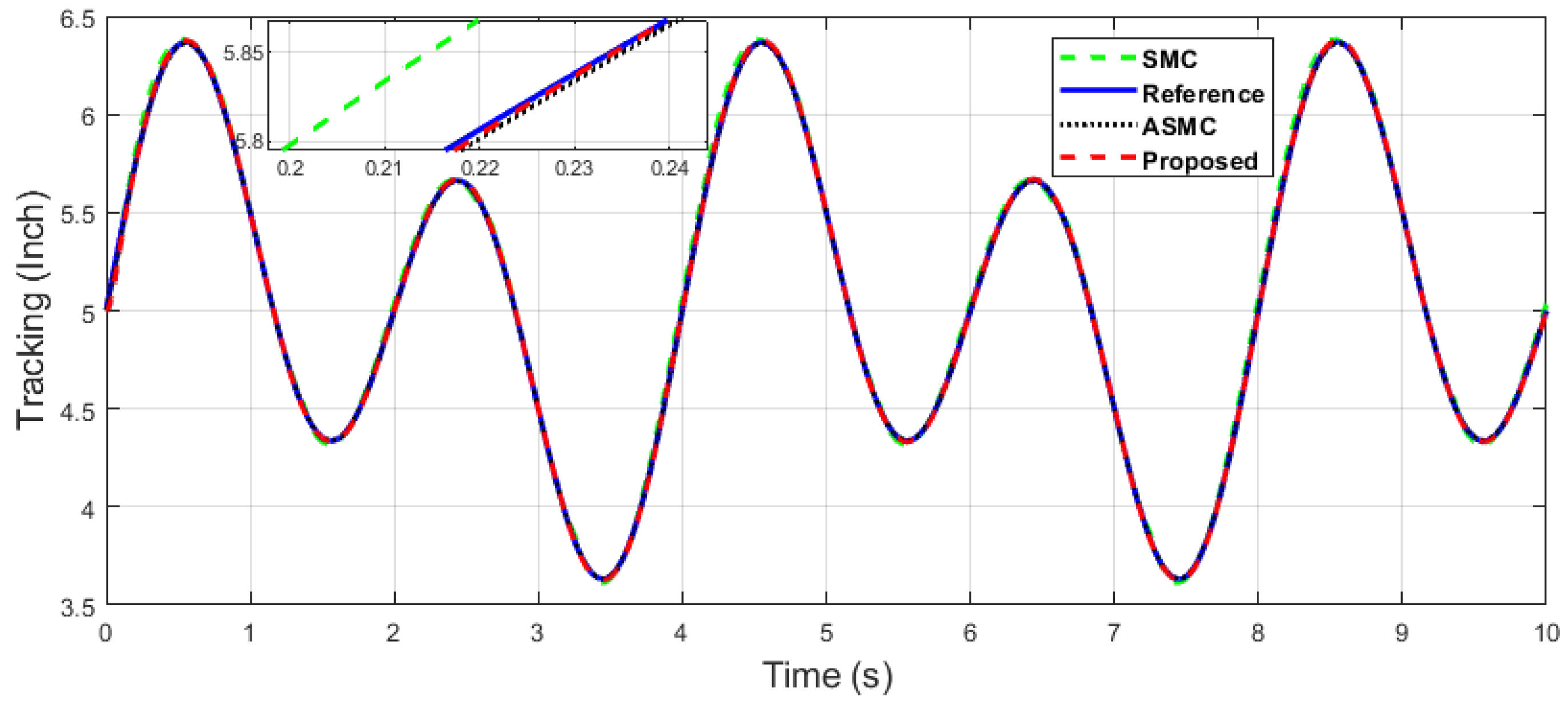
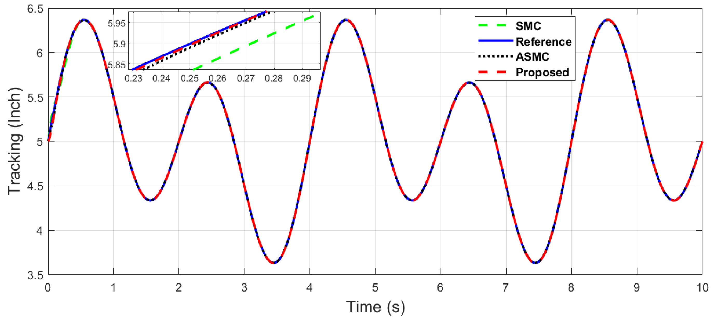
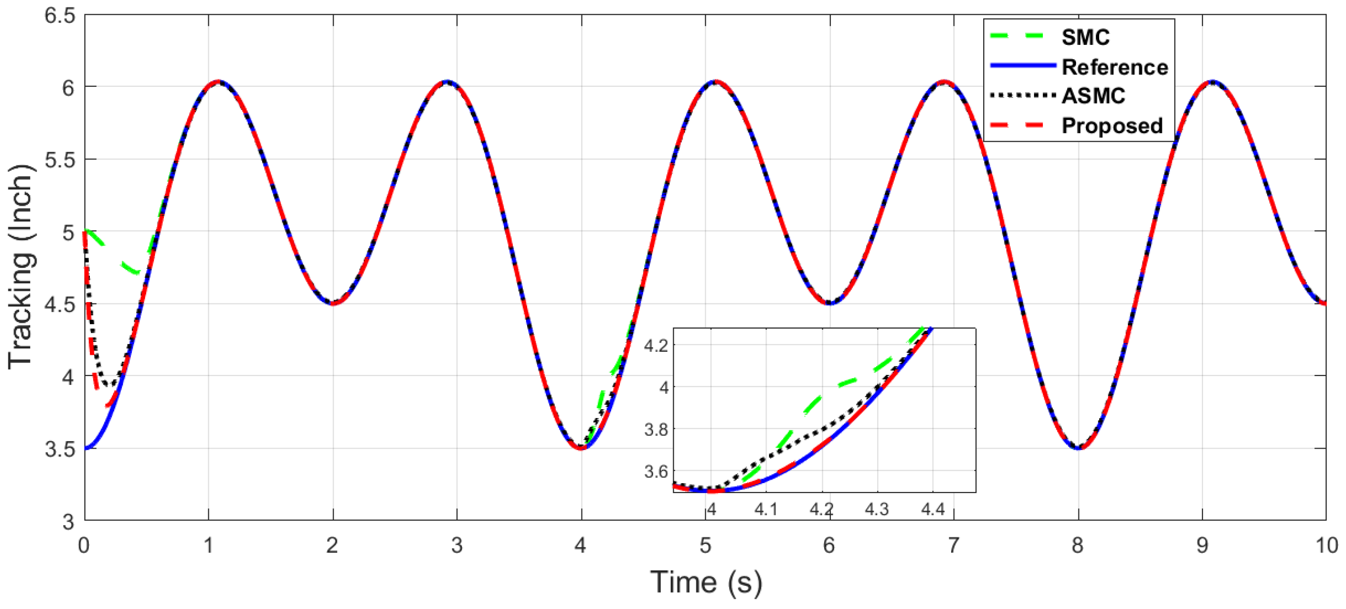
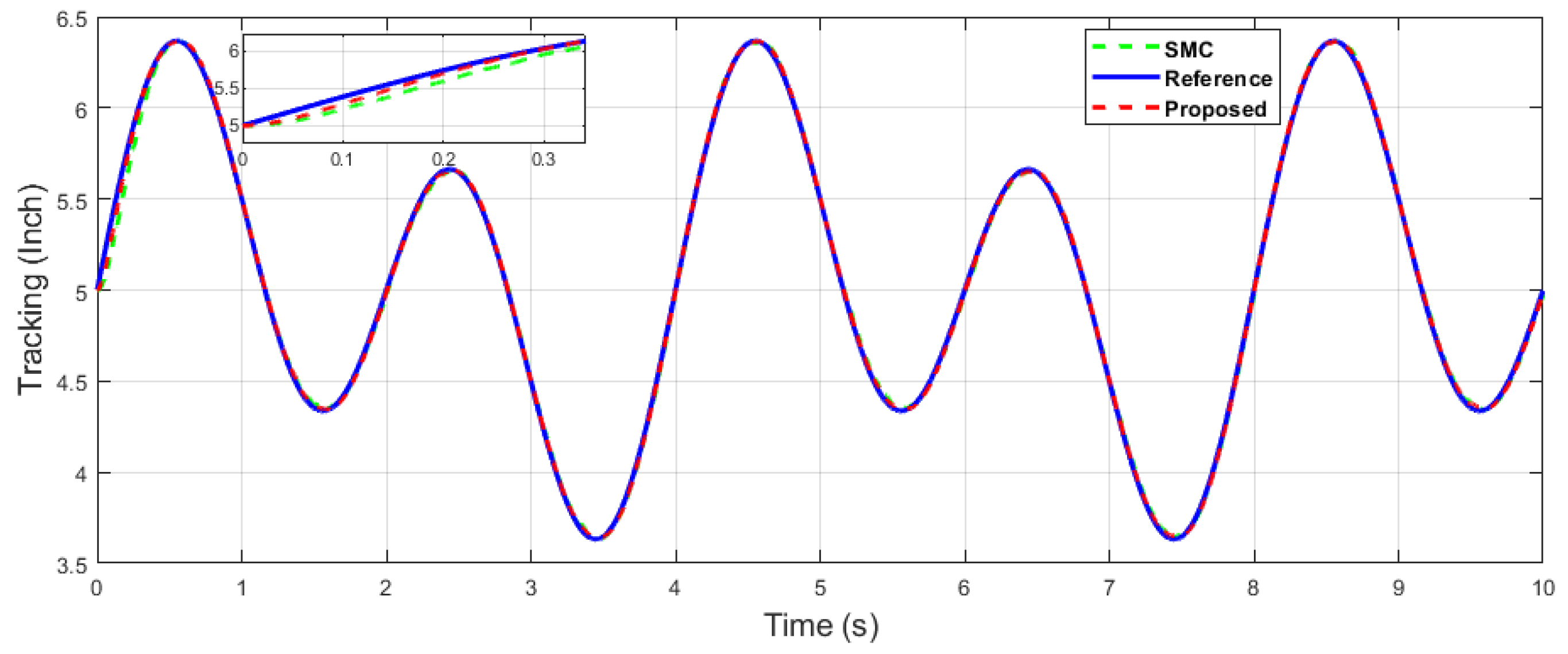
It can be seen in Figure 9 and Figure 10 that the proposed controller has overall fast convergence, as the PR control is the collaborative control along the X–Y axis in contrast to the SMC and ASMC, which depicts the superiority of the proposed algorithm.
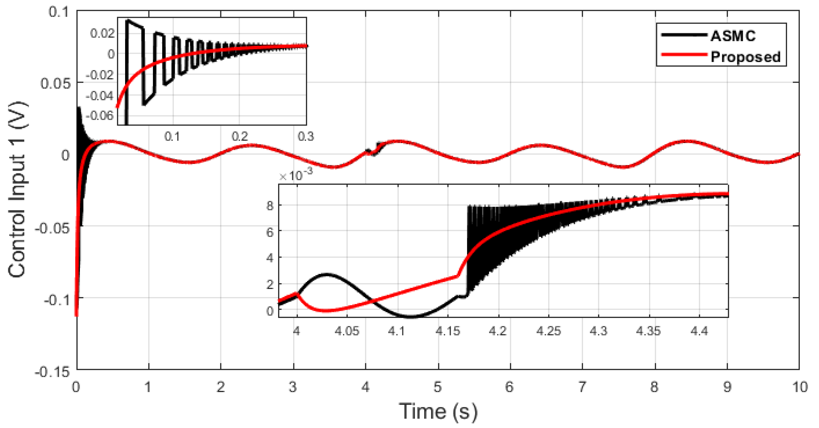
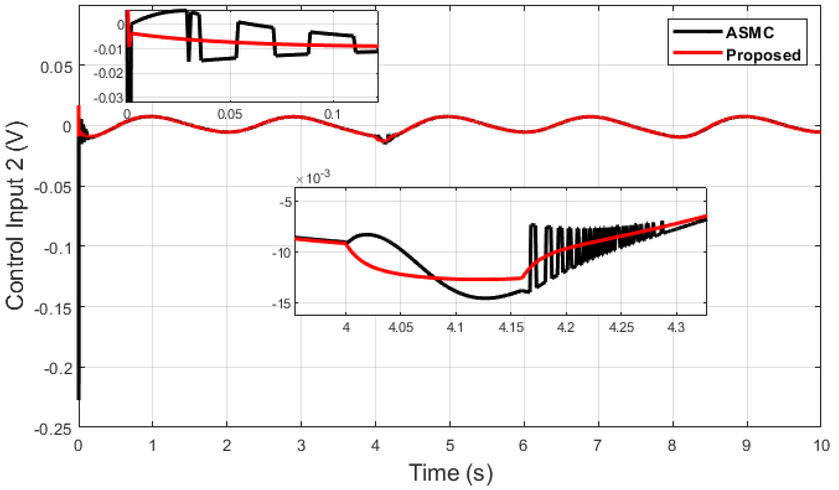
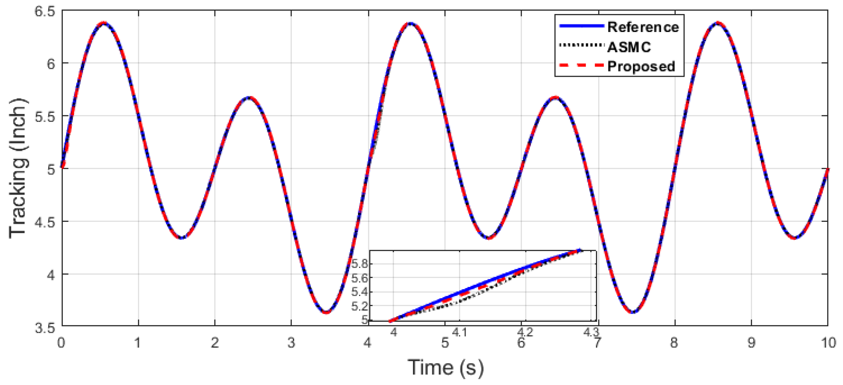
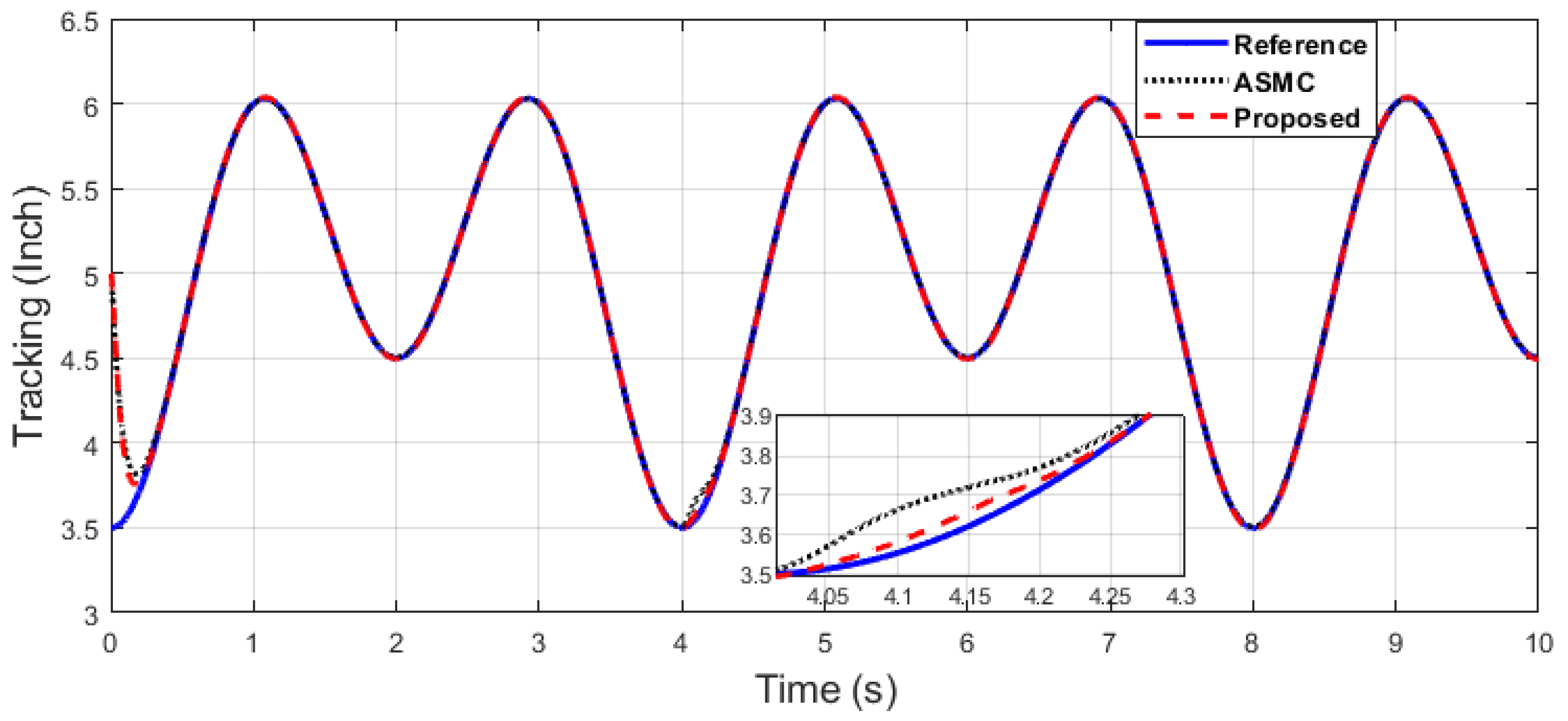
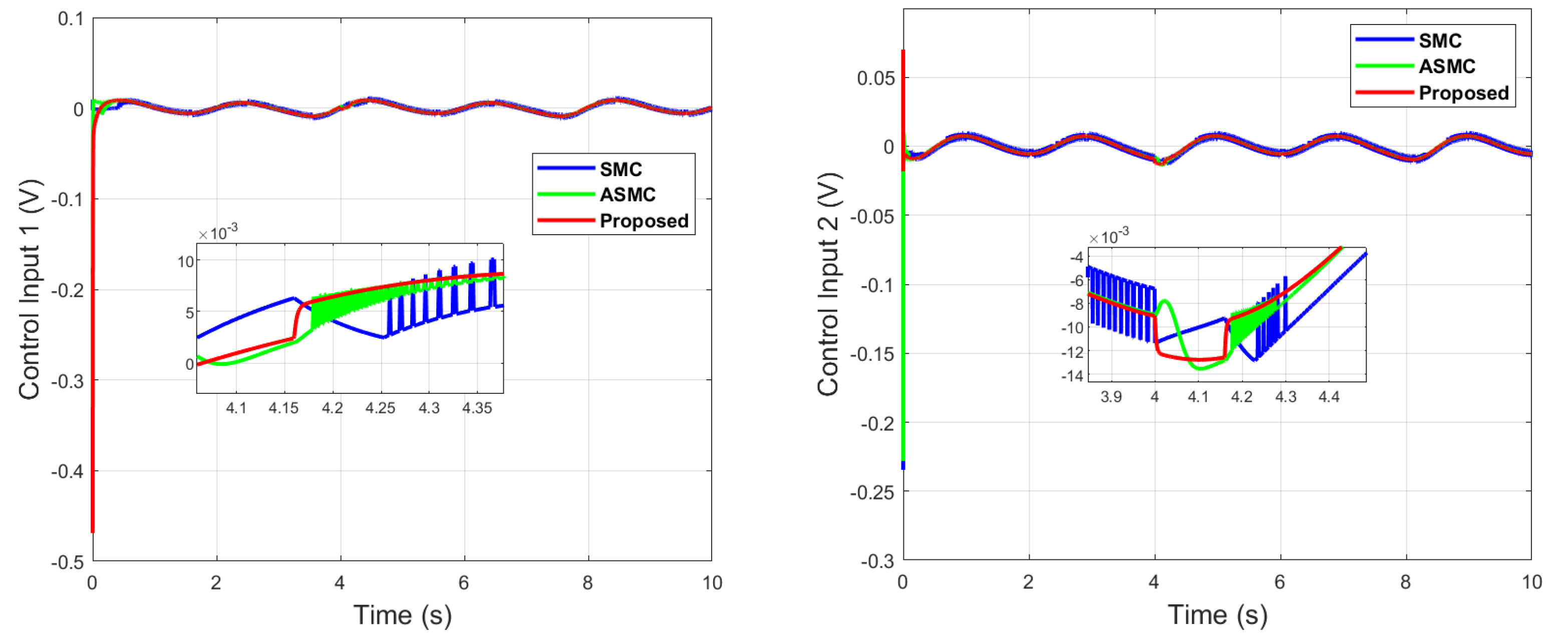
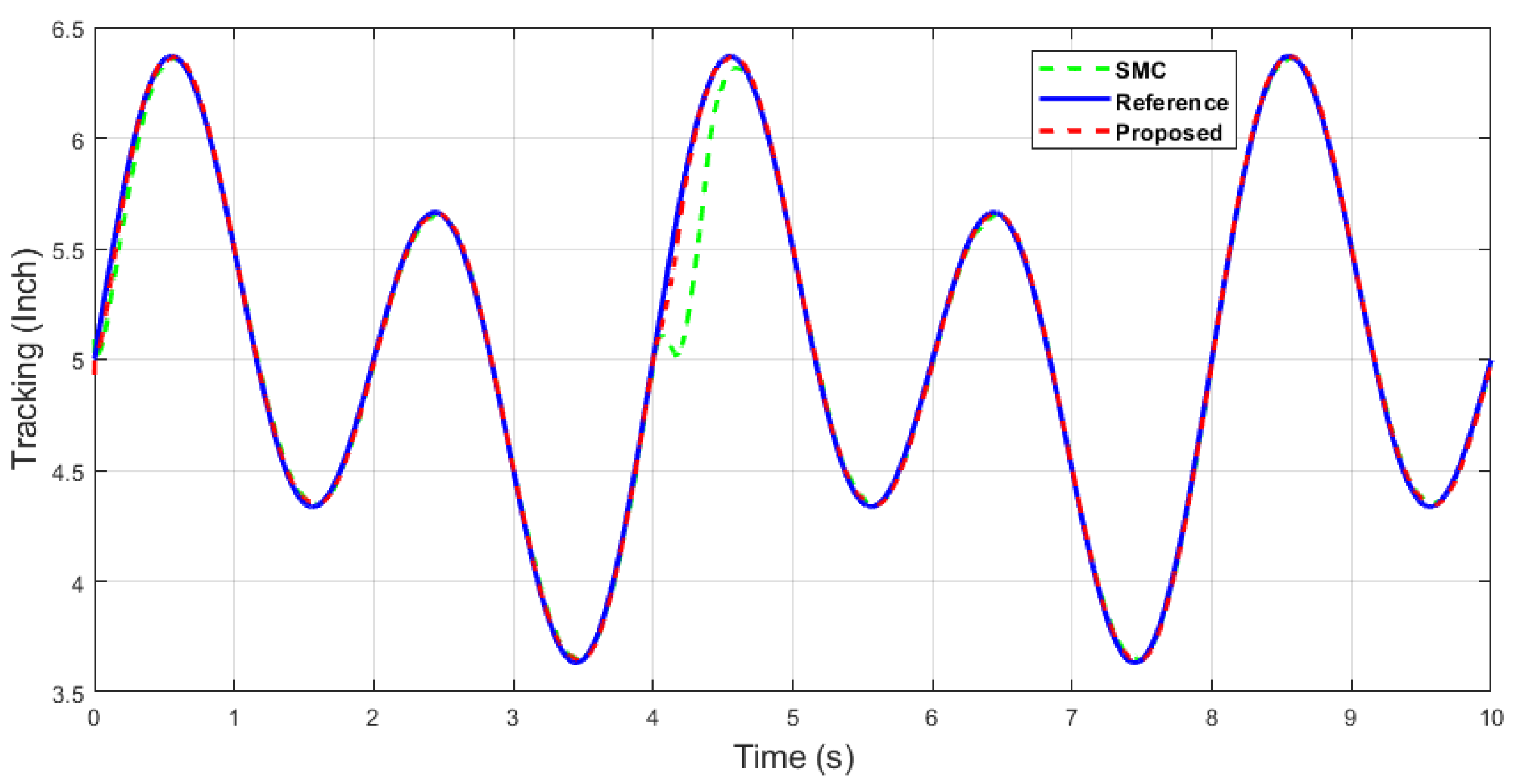
Next, an impulse disturbance is introduced with a magnitude of 0.2 V at 4 (s) for a short duration in the dual-sine-wave tracking to replicate in a real-world scenario if the robot is touched by a human or if any other sudden obstacle comes into contact with it during operation in order to consider uncertainty in the system. It can be seen from Figure 11, Figure 12, Figure 13 and Figure 14, which depict the comparative analysis with the ASMC [28], that when the system is subjected to impulse disturbance, the proposed control is robust with smooth control input when the disturbance is introduced at 4 (s), while the ASMC is prone to chattering in the initial phase, as well as during disturbance.
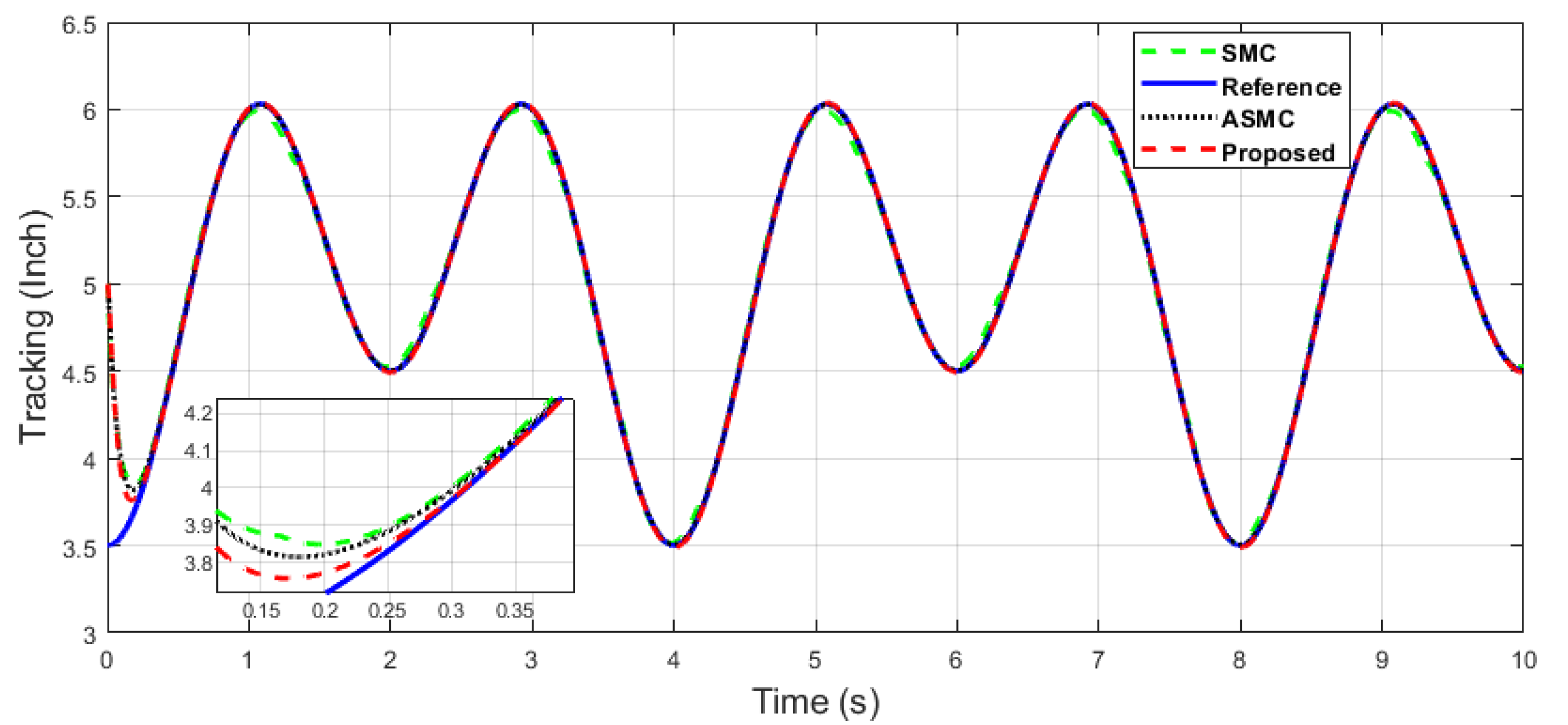
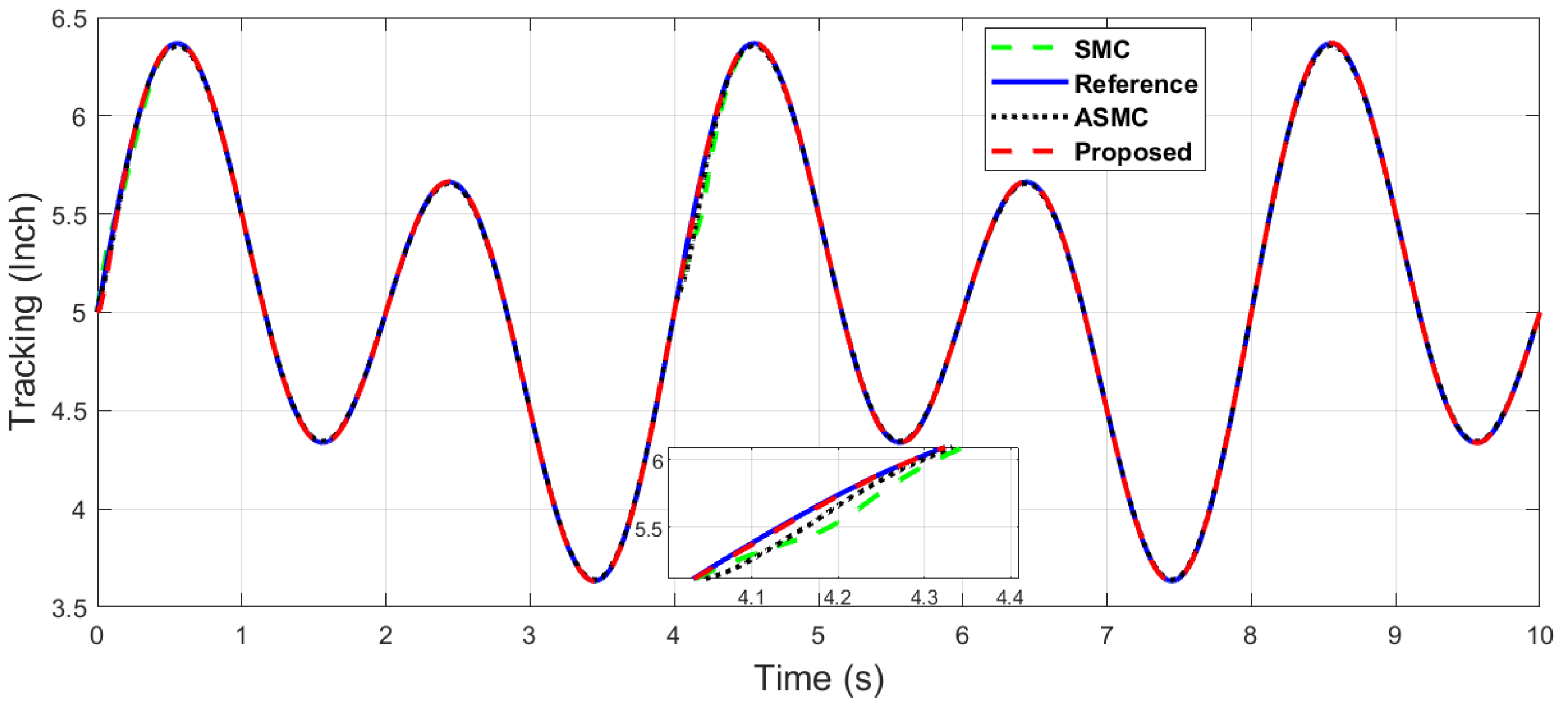
It can be seen in Figure 13 and Figure 14 that when an impulse disturbance is introduced at 4 (s), the proposed algorithm is robust in contrast to the ASMC, with better tracking and ability of disturbance rejection, which can be seen in the zoomed section of these figures.

4.2. Comparative Simulation with Optimal Tuning

In this section, the performance of all controllers with optimal parameter tuning is considered, in which the parameters of each controller are individually tuned to achieve less chattering, better tracking, and faster convergence. There is always a trade-off among chattering, fast convergence, and better tracking performance; thus, the control parameters are chosen as per Table 2 for the optimal tuning of all comparative algorithms.
The optimal tuning comparison is shown in Figure 15, Figure 16, Figure 17, Figure 18, Figure 19, Figure 20, Figure 21, Figure 22 and Figure 23.
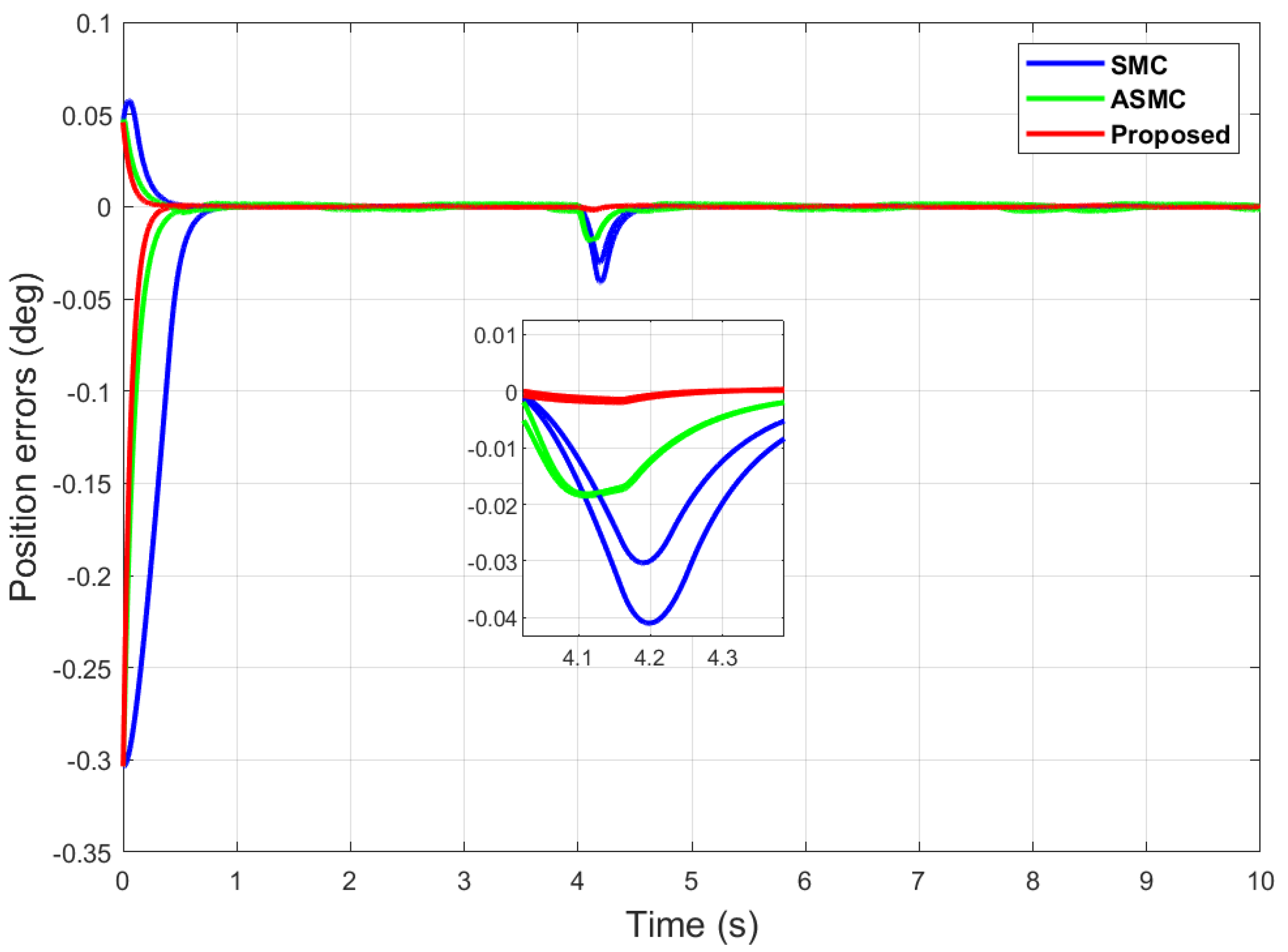
It can be seen in Figure 15 and Figure 16 that the proposed controller has overall fast convergence in contrast to the SMC and ASMC, which depicts the superiority of the proposed algorithm. In Figure 17, the proposed algorithm outperforms in terms of chattering reduction in contrast to the SMC and ASMC, which are prone to chattering, even in the case with individual optimal tuning.
Figure 18 and Figure 19 show the robustness of the proposed control, with overall fast convergence and better tracking performance compared with the SMC and ASMC, which can be seen in the zoomed sections of these figures.
Furthermore, an impulse disturbance is introduced with a magnitude of 0.2 V at 4 (s) for a short duration in dual-sine-wave tracking, similar to Section 4.1. Figure 20 shows the superiority of the proposed algorithm when subjected to an impulse disturbance.
It can be seen from Figure 21 that the comparative algorithms of the SMC and ASMC are prone to chattering when subjected to an impulse disturbance in contrast to the proposed control, which shows its superiority with much smoother control input.
It can be seen in Figure 22 and Figure 23, which show the optimal tuning comparison when an impulse disturbance is introduced at 4 (s), that the proposed algorithm is robust in contrast to the SMC and ASMC, with better tracking and ability of disturbance rejection, which can be seen in the zoomed section of these figures. The proposed control outperforms in the optimal tuning scenario.

5. Comparative Experimental Validation

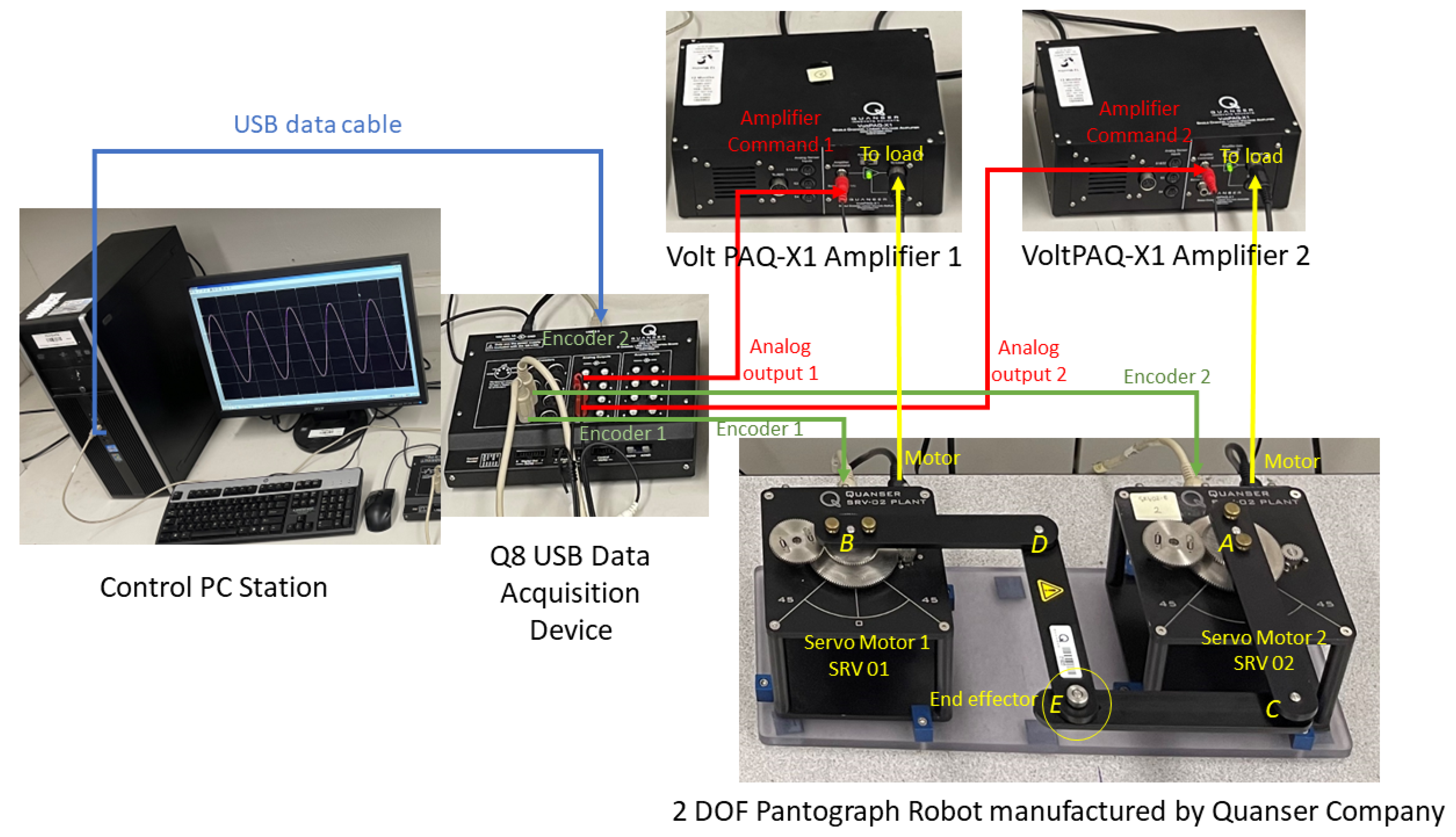
Hardware implementation was carried out on the 2 DOF pantograph robot. The experimental block diagram is shown below in Figure 24.
Real-time hardware experiments were carried out on the 2 DOF PR, manufactured by Quanser, with MATLAB and Quarc software. A detailed explanation is provided for ease to replicate the hardware results. From Figure 24, it can be seen that it consists of two servo motors, entitled S R V 01 and S R V 02 , connected with each other through four links such that it has three nonactuated and two actuated joints. Actuated joints with two links are mounted on S R V 01 and S R V 02 , on points A and B, respectively, at a fixed distance such that each link is 5 inches in length. From the PC, a USB cable is connected to a Q8 USB data acquisition device, which consists of two ports for Encoder 1 and 2, which are connected with both motors position measuring points. If the position of the motors is measured by the encoders of each servo motor and speed is not a known state of the system, then two state observers can be designed to estimate the speed and achieve better performance accordingly. The data acquisition device also comprises two ports for analog output 1 and 2, which are connected to two amplifiers, Volt FAQ-X1 Amplifier 1 and Volt FAQ-X1 Amplifier 2, respectively. By appropriately controlling the positions of both motors and link kinematics, the end-effector E position is controlled.
The control parameters for the proposed and comparative algorithms are selected as per Table 1. For the sake of fair comparison, common gains are taken as equal; moreover, the control input bandwidth is adjusted the same way for the proposed control and SMC.
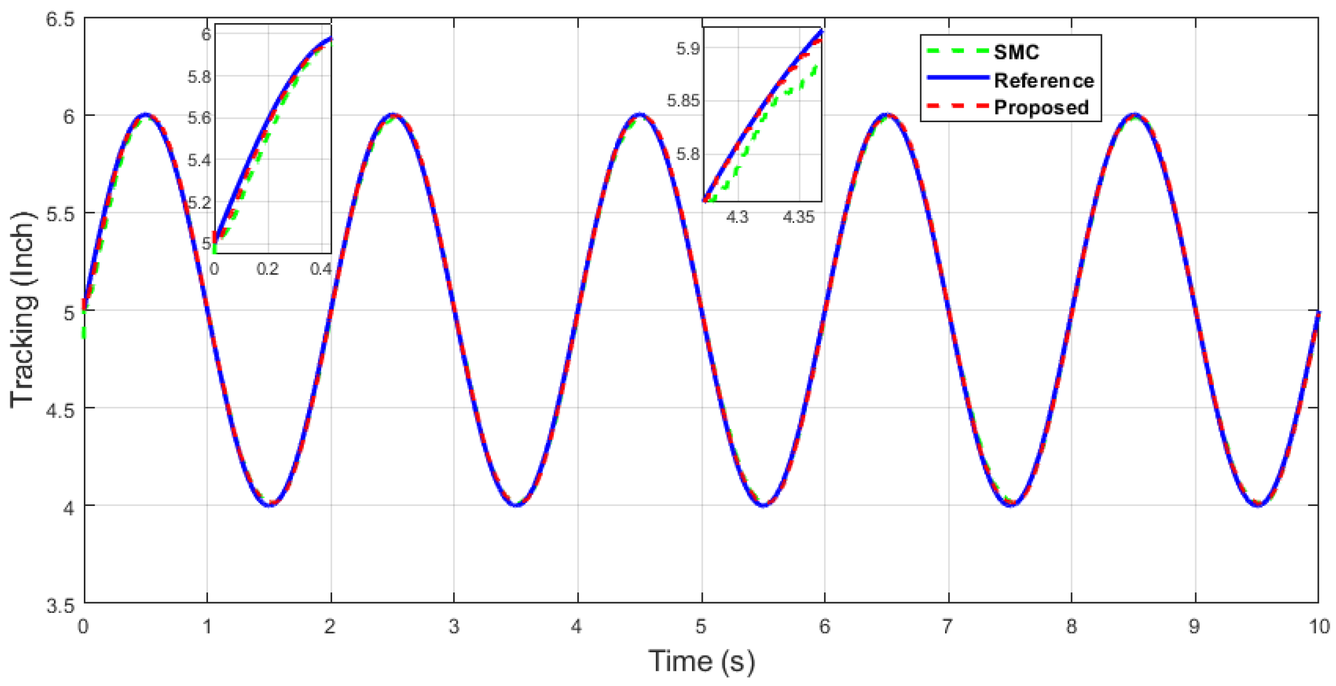
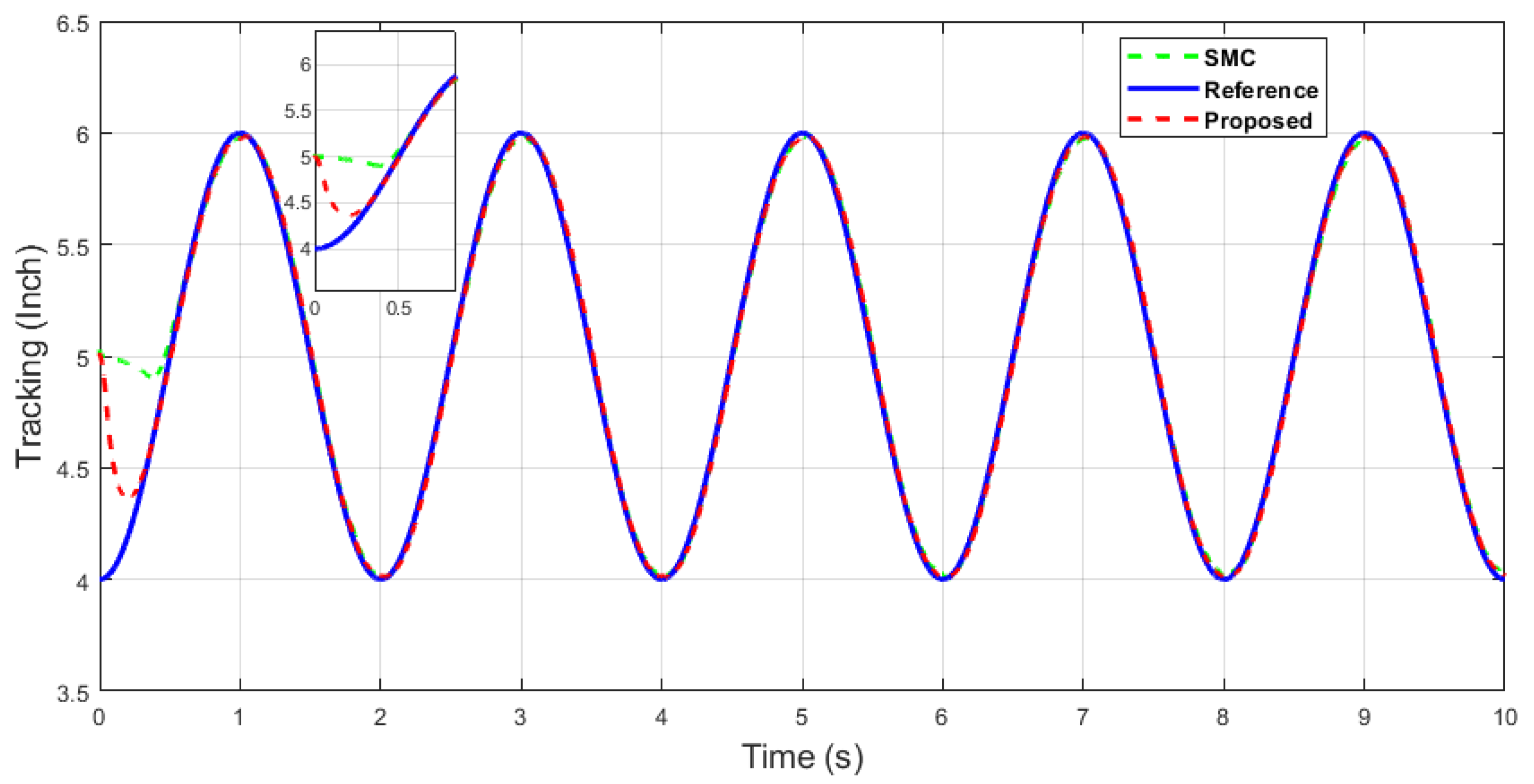
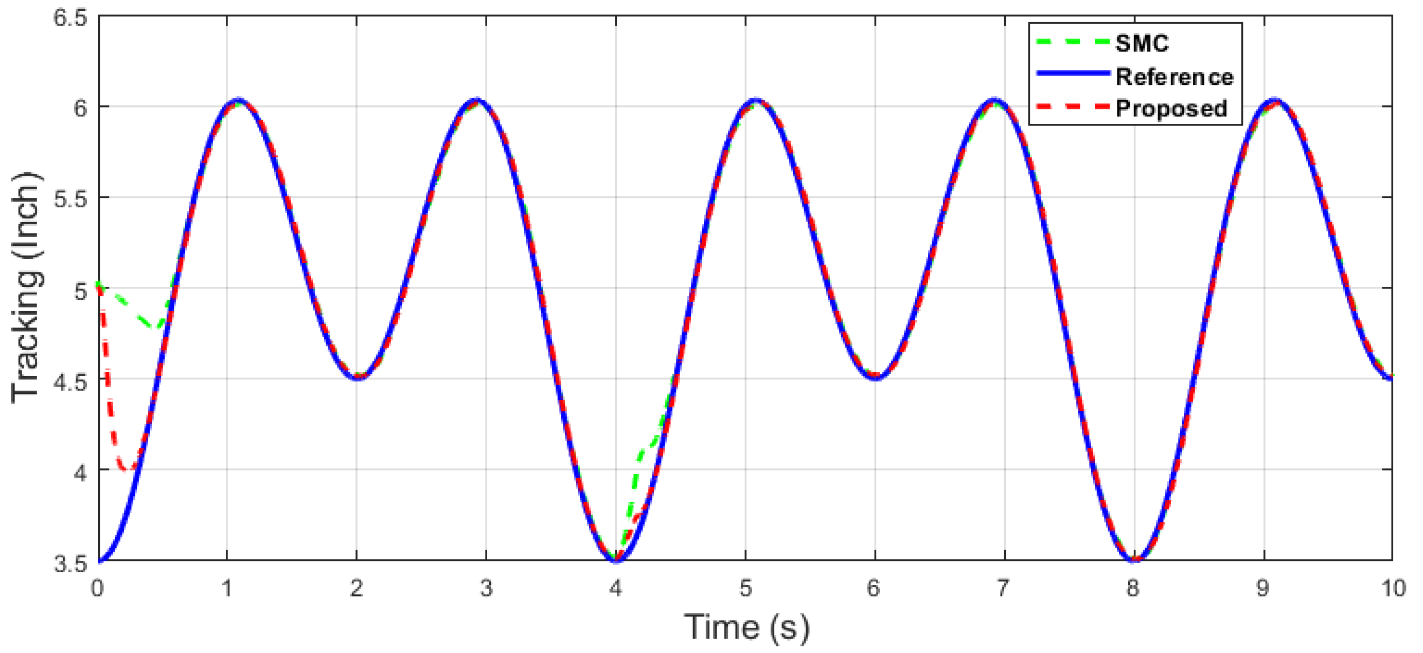
Three different cases for the experimental validation of the proposed control are carried out in Figure 25, Figure 26, Figure 27, Figure 28, Figure 29, Figure 30, Figure 31, Figure 32, Figure 33, Figure 34, Figure 35, Figure 36, Figure 37, Figure 38 and Figure 39. The first case includes the single-sine-wave tracking, and the second case deals with dual-sine-wave tracking, followed by dual-sine-wave tracking with an input disturbance introduced at 4 (s) for a short duration in the third case of the experimental validation.
Case 1 : Single-sine-wave tracking performance comparison and analysis for the PR.
In the first experiment, the PR tracks the simple sine wave along the x-axis as X E d = sin ( π t ) + 5 and the y-axis as Y E d = sin ( ( π t ) 0.5 π ) + 5 .
From Figure 25 and Figure 26, it can be seen that the proposed control is faster and has better tracking performance compared with the SMC, which is shown in the zoomed portions of the figures.
In the following case, dual-sine-wave tracking was also considered for both end-effector positions along the x- and y axes, respectively. The following results show the effectiveness of the proposed algorithm under dual-sine-wave tracking, as per Figure 30, Figure 31, Figure 32, Figure 33 and Figure 34.
Case 2 : Dual-sine-wave tracking comparison and analysis for the PR.
In the case of dual-sine-wave tracking, the following desired signal was given along the x-axis and the y-axis, respectively, i.e., X E d = sin ( π t ) + 0.5 sin ( π / 2 t ) + 5 and Y E d = sin ( π t ) 0.5 π + 0.5 sin ( π / 2 t 0.5 π ) + 5 .
Case 3 : Dual-sine-wave tracking under impulse disturbance with comparison and analysis for the PR.
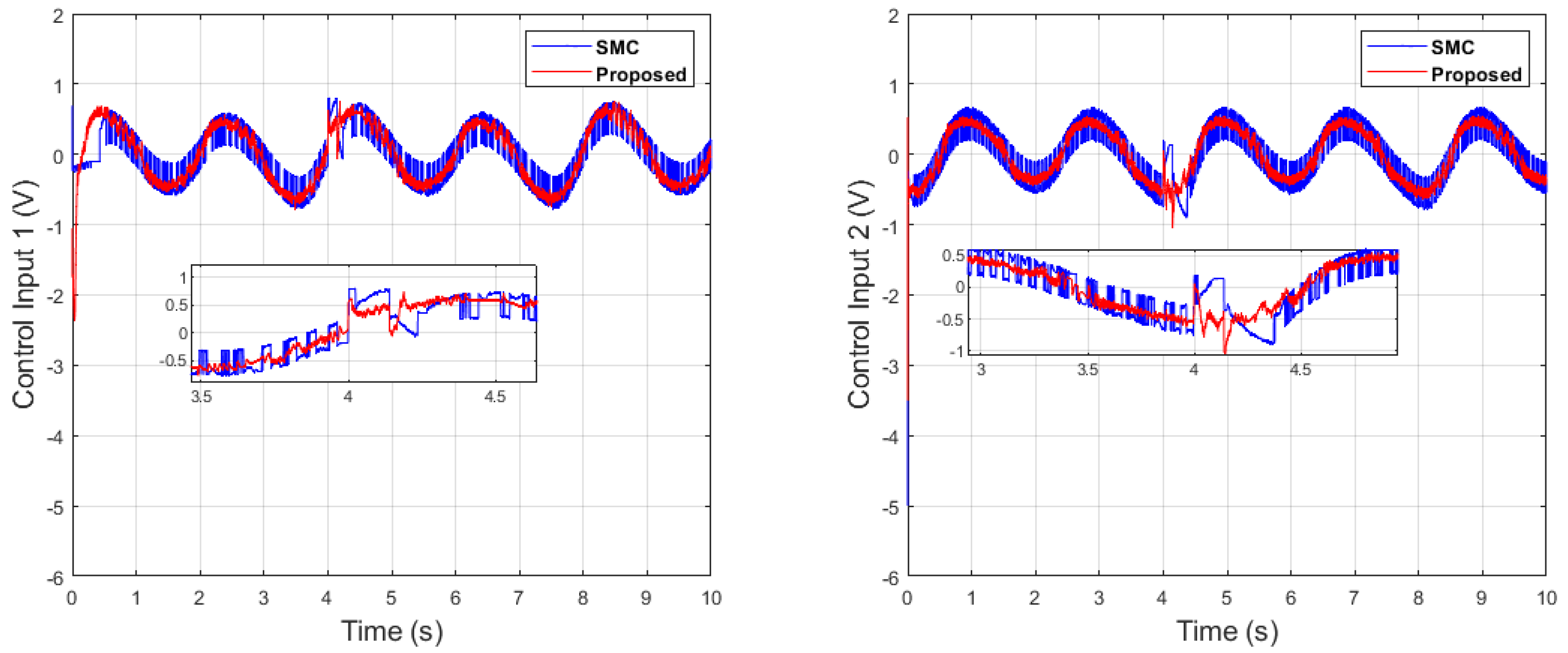
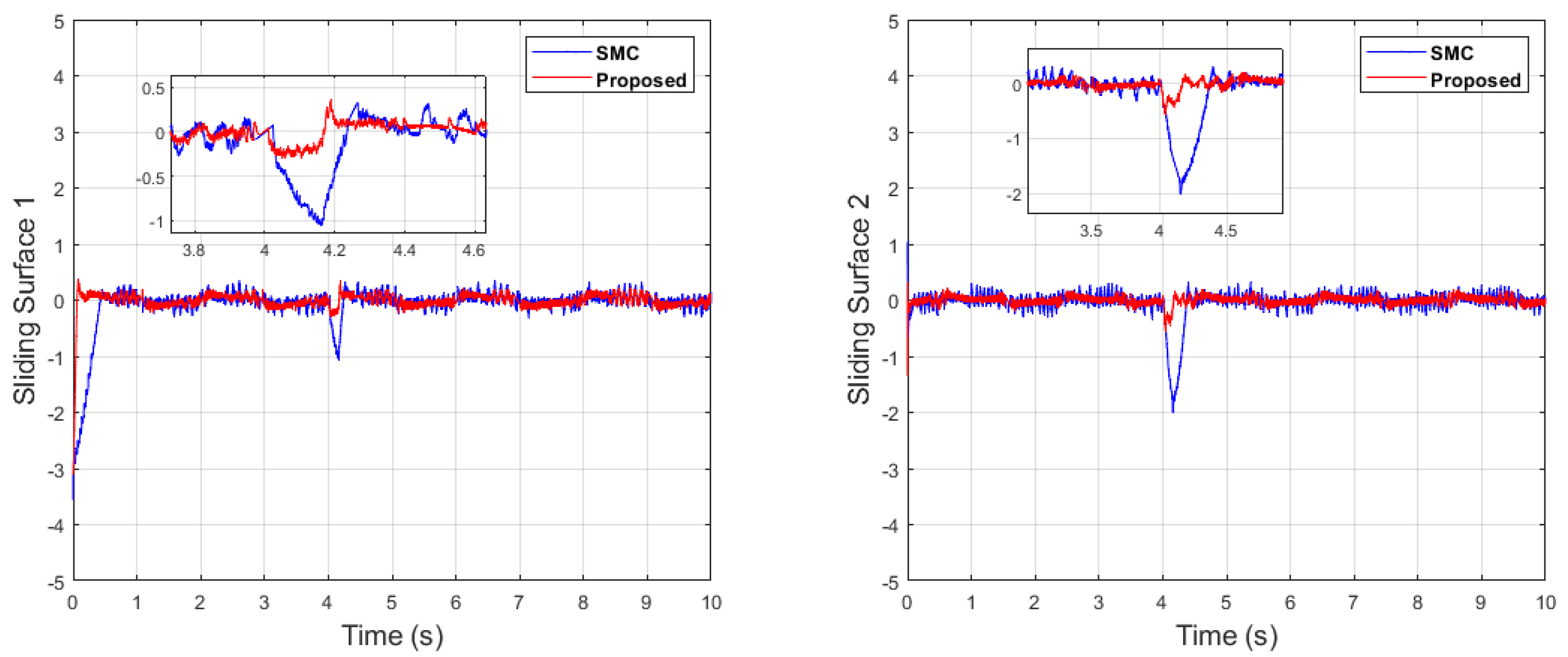
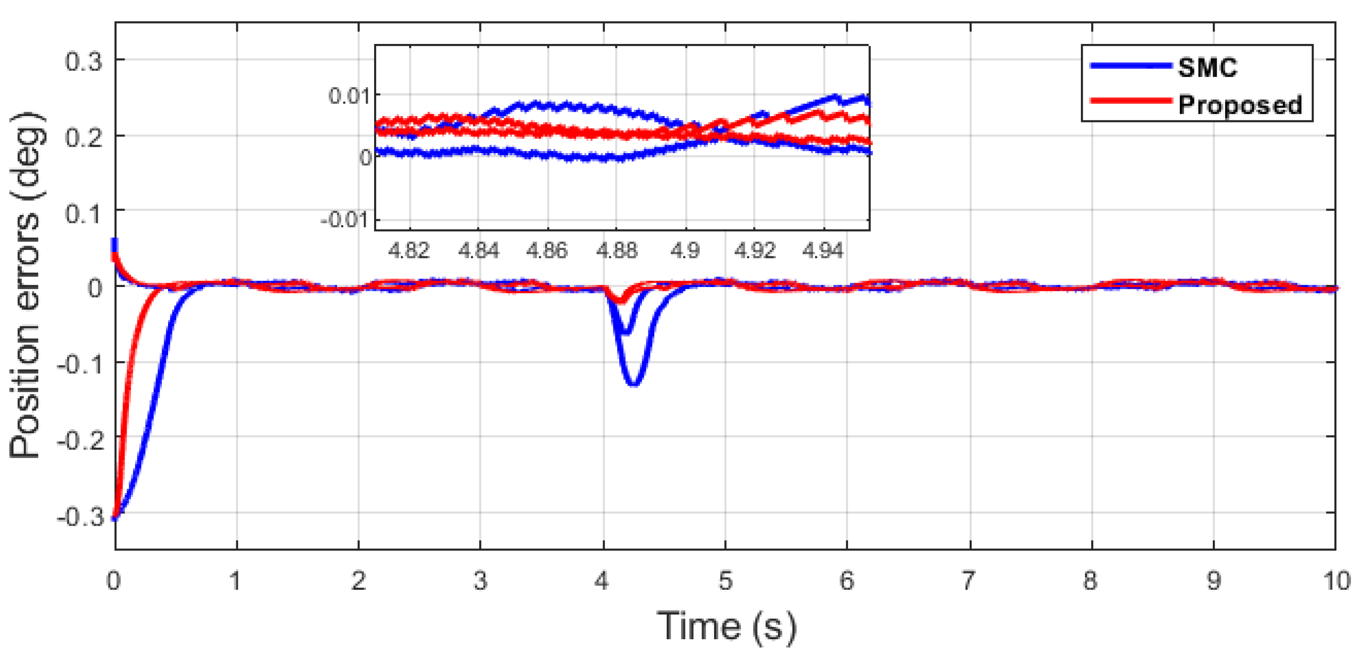
In the case of dual-sine-wave tracking under an impulse disturbance, the following desired signal was given along the x-axis and the y-axis, respectively, i.e., X E d = sin ( π t ) + 0.5 sin ( π / 2 t ) + 5 and Y E d = sin ( π t ) 0.5 π + 0.5 sin ( π / 2 t 0.5 π ) + 5 with an impulse disturbance of 0.2 V magnitude at 4 (s) for a short duration to consider the uncertainty in the system.

6. Discussion

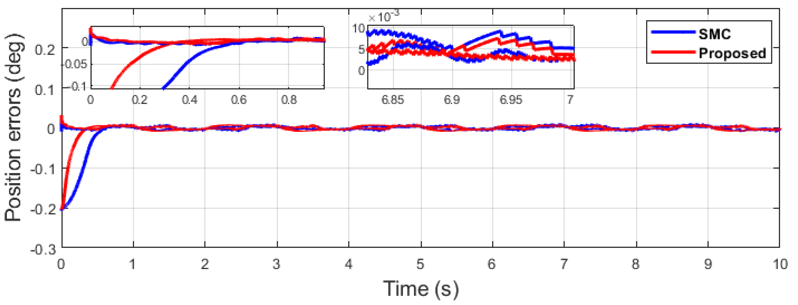
This section outlines the superiority of the proposed algorithm over the comparative algorithm by thorough discussion and in-depth analysis. Firstly, It can be seen from Figure 25, Figure 26, Figure 27, Figure 28 and Figure 29 that single-sine-wave tracking is achieved, which highlights the effectiveness of the proposed algorithm, as the position error e 1 of the proposed algorithm has significantly less value, i.e., RMS = 0.0177 in contrast to the SMC with an RMS = 0.0305, and position error e 2 has an RMS = 0.0032 compared with the SMC with an RMS = 0.0034, as shown in Table 3. Moreover, it can be seen from Figure 25 and Figure 26, in the zoomed subplot sections, that the proposed algorithm has fast convergence (0.3 s) compared with the comparative algorithm (0.6 s). In Figure 26, which represents the end-effector tracking along the y-axis, the convergence is significantly faster compared with Figure 25, which represents the end-effector tracking along the x-axis. The position control of the end-effector E of the pantograph robot has collaborative controlling coordinates, i.e., X E and Y E , as can be seen from Figure 37.
Remark 1.
End-effector position control is the collaborative position control along the X–Y axis; thus, the overall convergence of position errors is faster in the proposed algorithm compared with the SMC.
Figure 27 depicts the control input comparison of the proposed algorithm and SMC by single sine wave, and a significant reduction in chattering magnitude can be seen. The sliding surface comparison of single sine wave shows that from Figure 28, the proposed algorithm’s sliding surface convergence is faster to origin, with a reduction in chattering magnitude. A similar trend can be seen in Case 2 of dual-sine-wave tracking from Figure 30, Figure 31, Figure 32, Figure 33 and Figure 34, with the position error e 1 of the proposed algorithm having significantly less value, i.e., RMS = 0.0272 in contrast to the SMC with RMS = 0.0472, and position error e 2 has an RMS = 0.0038 compared with the SMC with an RMS = 0.0039, as shown in Table 3. This is due to the trade-off between convergence and tracking error. Furthermore, it can be seen from Figure 34, in the zoomed subplot sections, that the proposed algorithm has fast convergence (0.3 s) compared with the comparative algorithm (0.6 s). A reduction in chattering magnitude can also be seen in Figure 32. As previously mentioned, the end-effector E has collaborative position control coordinates along the X–Y axis; thus, the overall effect of the proposed algorithm errors convergence is faster. In the case of dual-sine-wave tracking, the proposed algorithm outperforms with faster convergence, less steady-state error, and improved tracking performance.
Similarly, it can be seen in Case 3 of dual-sine-wave tracking from Figure 35, Figure 36, Figure 37, Figure 38 and Figure 39 that the position error e 1 of the proposed algorithm has less RMS value, i.e., RMS = 0.0272 in contrast to the SMC with an RMS = 0.0478, and position error e 2 has significantly less RMS = 0.0047 compared with the SMC, with an RMS = 0.0196, as shown in Table 3. This shows the superiority of the proposed algorithm to handle the external disturbances and uncertainties in the system with better tracking performance and ability of disturbance rejection. In case of impulse disturbance, the SMC has a significantly large error e 2 , i.e., RMS = 0.0196, which shows its drawback in this regard.
Remark 2.
The proposed control has broad applications in robotics and can be used for various second-order systems such as pick and place robots, robotic hands, throttle valves, DC motors, etc.

7. Conclusions

A robust controller that functions in a closed-loop domain with faster convergence is indispensable in various sectors like robotics, space engineering, mining industry, advanced manufacturing sector, agriculture sector, etc. The sliding mode controller (SMC) has proven to be a robust controller in the case of external disturbances, nonlinearities, uncertainties, and modeled system dynamics. In this article, a novel improved SMC based on the S e c h function has been proposed that achieves fast convergence, reduced chattering, and has less steady-state error. For the stability analysis, the Lyapunov stability criteria were utilized. Simulations and experimental implementations were carried out on a PR, showing the effectiveness of the proposed algorithm. The work proposed in this paper is focused on asynchronous control, in which the position errors are converging at different time spans. Thus, future work will consider synchronous control, in which both position errors will converge at the same time, which will make the system energy efficient.

Author Contributions

Conceptualization, M.A.H.; methodology, M.A.H. and Z.C.; software, M.A.H. and Z.C.; validation, M.A.H.; formal analysis, M.A.H. and Z.C.; investigation, Z.C.; resources, Z.M.; data curation, Z.C. and Z.M.; writing—original draft preparation, M.A.H. and Z.C.; writing—review and editing, M.A.H., Z.C. and Z.M.; visualization, M.A.H.; supervision, Z.C. and Z.M.; project administration, Z.C. and Z.M.; funding acquisition, Z.C. and Z.M. All authors have read and agreed to the published version of the manuscript.

Funding

This work was supported in part by the Australian Research Council under grant number DP190101557.

Data Availability Statement

Not applicable.

Acknowledgments

We would like to acknowledge the support of Jyoti Mishra and other lab mates who helped either at the administrative level or technical side, without whom we would not have been able to complete this work.

Conflicts of Interest

The authors declare no conflict of interest.

References

  1. Cheah, C.C.; Li, X.; Yan, X.; Sun, D.T. Simple PD control scheme for robotic manipulation of biological cell. IEEE Trans. Autom. Control 2014, 60, 1427–1432. [Google Scholar] [CrossRef]
  2. Awan, Z.S.; Ali, K.; Iqbal, J.; Mehmood, A. Adaptive backstepping based sensor and actuator fault tolerant control of a manipulator. J. Electr. Eng. Technol. 2019, 14, 2497–2504. [Google Scholar] [CrossRef]
  3. Al-Mahturi, A.; Wahid, H. Optimal tuning of linear quadratic regulator controller using a particle swarm optimization for two-rotor aerodynamical system. Int. J. Electron. Commun. Eng. 2017, 11, 184–190. [Google Scholar]
  4. Feng, H.; Yin, C.B.; Weng, W.W.; Ma, W.; Zhou, J.J.; Jia, W.H.; Zhang, Z.L. Robotic excavator trajectory control using an improved GA based PID controller. Mech. Syst. Signal Process. 2018, 105, 153–168. [Google Scholar] [CrossRef]
  5. Ali, N.; Ayaz, Y.; Iqbal, J. Collaborative position control of pantograph robot using particle swarm optimization. Int. J. Control Autom. Syst. 2022, 20, 198–207. [Google Scholar] [CrossRef]
  6. Saisudha, V.; Seeja, G.; Pillay, R.V.; Manikutty, G.; Bhavani, R.R. Analysis of speed control of DC motor using LQR method. Int. J. Control Theory Appl. 2016, 15, 7377–7385. [Google Scholar]
  7. Zheng, X.; Su, X. Sliding mode control of electro-hydraulic servo system based on optimization of quantum particle swarm algorithm. Machines 2021, 9, 283. [Google Scholar] [CrossRef]
  8. Young, K.D.; Utkin, V.I.; Ozguner, U. A control engineer’s guide to sliding mode control. IEEE Trans. Control Syst. Technol. 1999, 7, 328–342. [Google Scholar] [CrossRef]
  9. Šabanovic, A. Variable structure systems with sliding modes in motion control. Int. J. Control Theory Appl. 2011, 7, 212–223. [Google Scholar] [CrossRef]
  10. Utkin, V.; Guldner, J.; Shi, J. Sliding Mode Control in Electro-Mechanical Systems, 2nd ed.; CRC Press: Boca Raton, FL, USA, 2017; pp. 154–503. [Google Scholar]
  11. Utkin, V.; Lee, H. Chattering problem in sliding mode control systems. IEEE Proc. Int. Workshop Var. Struct. Syst. 2006, 46, 346–350. [Google Scholar]
  12. Hassan, M.A.; Cao, Z.; Man, Z. End Effector Position Control of Pantograph Type Robot Using Sliding Mode Controller. In Proceedings of the Australian and New Zealand Control Conference, Gold Coast, Australia, 25 November 2022; pp. 156–160. [Google Scholar]
  13. Levant, A. Universal single-input-single-output (SISO) sliding-mode controllers with finite-time convergence. IEEE Trans. Autom. Control. 2001, 46, 1447–1451. [Google Scholar] [CrossRef]
  14. Utkin, V.; Poznyak, A.; Orlov, Y.; Polyakov, A. Conventional and high order sliding mode control. J. Frankl. Inst. 2020, 357, 10244–10261. [Google Scholar] [CrossRef]
  15. Bartolini, G.; Ferrara, A.; Usai, E.; Utkin, V.I. On multi-input chattering-free second-order sliding mode control. IEEE Trans. Autom. Control 2000, 45, 1711–1717. [Google Scholar] [CrossRef]
  16. Kawamura, A.; Itoh, H.; Sakamoto, K. Sakamoto, Chattering reduction of disturbance observer based sliding mode control. IEEE Trans. Ind. Appl. 1994, 30, 456–461. [Google Scholar] [CrossRef]
  17. Xu, W.; Jiang, Y.; Mu, C. Novel composite sliding mode control for PMSM drive system based on disturbance observer. IEEE Trans. Appl. Supercond. 2016, 26, 1–5. [Google Scholar] [CrossRef]
  18. Kachroo, P.; Tomizuka, M. Chattering reduction and error convergence in the sliding mode control of a class of nonlinear systems. IEEE Trans. Autom. Control 1996, 41, 1063–1068. [Google Scholar] [CrossRef]
  19. Gao, W.; Hung, J.C. Variable structure control of nonlinear systems: A new approach. IEEE Trans. Ind. Electron. 1993, 40, 45–55. [Google Scholar]
  20. Bartoszewicz, A. Discrete-time quasi-sliding-mode control strategies. IEEE Trans. Ind. Electron. 1998, 45, 633–637. [Google Scholar] [CrossRef]
  21. Bartoszewicz, A.; Leśniewski, P. New switching and nonswitching type reaching laws for SMC of discrete time systems. IEEE Trans. Control Syst. Technol. 2015, 24, 670–677. [Google Scholar] [CrossRef]
  22. Fallaha, C.; Saad, M.; Kanaan, H.; Al-Hadded, K. Sliding-mode control with exponential reaching law. IEEE Trans. Ind. Electron. 2011, 58, 600–610. [Google Scholar] [CrossRef]
  23. Bartoszewicz, A. A new reaching law for sliding mode control of continous time systems with constraints. Trans. Inst. Meas. Control 2014, 37, 515–521. [Google Scholar] [CrossRef]
  24. Zhai, J.; Li, Z. Fast-exponential sliding mode control of robotic manipulator with super-twisting method. IEEE Trans. Circuits Syst. II Express Briefs 2021, 69, 489–493. [Google Scholar] [CrossRef]
  25. Hou, H.; Yu, X.; Xu, L.; Rsetam, K.; Cao, Z. Finite-time continuous terminal sliding mode control of servo motor systems. IEEE Trans. Ind. Electron. 2019, 67, 5647–5656. [Google Scholar] [CrossRef]
  26. Mobayen, S.; Alattas, K.A.; Assawinchaichote, W. Adaptive continuous barrier function terminal sliding mode control technique for disturbed robotic manipulator. IEEE Trans. Circuits Syst. I Regul. Pap. 2021, 68, 4403–4412. [Google Scholar] [CrossRef]
  27. Yang, T.; Deng, Y.; Li, H.; Sun, Z.; Cao, H.; Wei, Z. Fast integral terminal sliding mode control with a novel disturbance observer based on iterative learning for speed control of PMSM. ISA Trans. 2023, 134, 460–471. [Google Scholar] [CrossRef] [PubMed]
  28. Nguyen, T.H.; Nguyen, T.T.; Nguyen, V.Q.; Le, K.M.; Tran, H.N.; Jeon, J.W. An adaptive sliding mode controller with a modified reduced-order PI observer for speed regulation of a permanent magnet synchronous motor. IEEE Trans. Ind. Electron. 2022, 69, 7181–7191. [Google Scholar] [CrossRef]
  29. Wang, H.; Liu, Z.; Han, Z.; Wu, Y.; Liu, D. Rapid Adaptation for Active Pantograph Control in High-Speed Railway via Deep Meta Reinforcement Learning. IEEE Trans. Cybern. 2023, 1–13. [Google Scholar] [CrossRef]
  30. Bahraini, M.S.; Mahmoodabadi, M.J.; Lohse, N. Robust Adaptive Fuzzy Fractional Control for Nonlinear Chaotic Systems with Uncertainties. Fractal Fract. 2023, 7, 484. [Google Scholar] [CrossRef]
  31. Dong, H.; Yang, X.; Gao, H.; Yu, X. Practical Terminal Sliding-Mode Control and Its Applications in Servo Systems. IEEE Trans. Ind. Electron. 2023, 70, 752–761. [Google Scholar] [CrossRef]
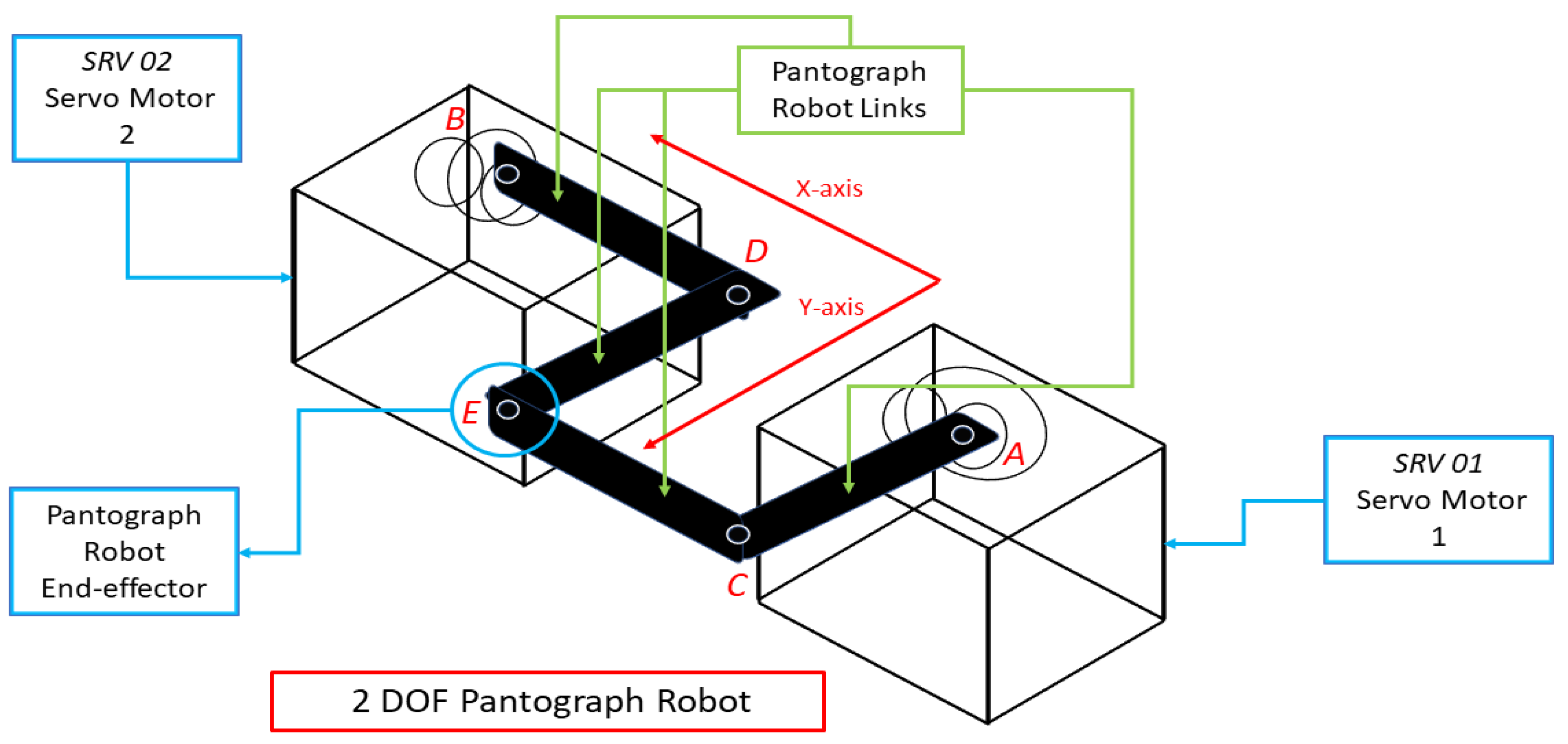
Figure 1. Pantograph robot.
Machines 11 00941 g001
Figure 2. Forward kinematics for the four links of the pantograph robot [12].
Machines 11 00941 g002
Figure 3. Inverse kinematics for the four links of the pantograph robot [12].
Machines 11 00941 g003
Figure 4. The proposed PR control structure.
Machines 11 00941 g004
Figure 5. Hyperbolic secant function graphical representation.
Machines 11 00941 g005
Figure 6. Position error comparison of dual sine wave.
Machines 11 00941 g006
Figure 7. Sliding surfaces comparison of dual sine wave.
Machines 11 00941 g007
Figure 8. Control inputs comparison of dual sine wave.
Machines 11 00941 g008
Figure 9. The x-axis end-effector tracking of dual sine wave.
Machines 11 00941 g009
Figure 10. The y-axis end-effector tracking of dual sine wave.
Machines 11 00941 g010
Figure 11. Control input 1 comparison of dual sine wave under impulse disturbance introduced at 4 (s).
Machines 11 00941 g011
Figure 12. Control input 2 comparison of dual sine wave under impulse disturbance introduced at 4 (s).
Machines 11 00941 g012
Figure 13. The x-axis end-effector tracking of dual sine wave under impulse disturbance introduced at 4 (s).
Machines 11 00941 g013
Figure 14. The y-axis end-effector tracking of dual sine wave under impulse disturbance introduced at 4 (s).
Machines 11 00941 g014
Figure 15. Position error comparison of dual sine wave with optimal tuning.
Machines 11 00941 g015
Figure 16. Sliding surface comparison of dual sine wave with optimal tuning.
Machines 11 00941 g016
Figure 17. Control inputs comparison of dual sine wave with optimal tuning.
Machines 11 00941 g017
Figure 18. The x-axis end-effector tracking of dual sine wave with optimal tuning.
Machines 11 00941 g018
Figure 19. The y-axis end-effector tracking of dual sine wave with optimal tuning.
Machines 11 00941 g019
Figure 20. Position error comparison of dual sine wave with optimal tuning when subjected to an impulse disturbance at 4 (s).
Machines 11 00941 g020
Figure 21. Control input comparison of dual sine wave with optimal tuning when subjected to an impulse disturbance at 4 (s).
Machines 11 00941 g021
Figure 22. The x-axis end-effector tracking of dual sine wave with optimal tuning when subjected to an impulse disturbance at 4 (s).
Machines 11 00941 g022
Figure 23. The y-axis end-effector tracking of dual sine wave with optimal tuning when subjected to an impulse disturbance at 4 (s).
Machines 11 00941 g023
Figure 24. Quanser 2 DOF PR hardware implementation setup in the robotics lab.
Machines 11 00941 g024
Figure 25. The x-axis end-effector tracking of single sine wave.
Machines 11 00941 g025
Figure 26. The y-axis end-effector tracking of single sine wave.
Machines 11 00941 g026
Figure 27. Control inputs comparison of single sine wave.
Machines 11 00941 g027
Figure 28. Sliding surfaces comparison of single sine wave.
Machines 11 00941 g028
Figure 29. Position errors comparison of single sine wave.
Machines 11 00941 g029
Figure 30. The x-axis end-effector tracking of dual sine wave.
Machines 11 00941 g030
Figure 31. The y-axis end-effector tracking of dual sine wave.
Machines 11 00941 g031
Figure 32. Control input comparison of dual sine wave.
Machines 11 00941 g032
Figure 33. Sliding surface comparison of dual sine wave.
Machines 11 00941 g033
Figure 34. Position error comparison of dual sine wave.
Machines 11 00941 g034
Figure 35. The x-axis end-effector tracking of dual sine wave under impulse disturbance introduced at 4 (s).
Machines 11 00941 g035
Figure 36. The y-axis end-effector tracking of dual sine wave under impulse disturbance introduced at 4 (s).
Machines 11 00941 g036
Figure 37. Control input comparison of dual sine wave under impulse disturbance introduced at 4 (s).
Machines 11 00941 g037
Figure 38. Sliding surface comparison of dual sine wave under impulse disturbance introduced at 4 (s).
Machines 11 00941 g038
Figure 39. Position error comparison of dual sine wave under impulse disturbance introduced at 4 (s).
Machines 11 00941 g039
Table 1. Control parameters for experimental analysis.
ControllerController Parameters
SMC K m = 1.53  (rad/sV), K = 14 , T m = 0.0254  (s),
λ = 14 , L = 5  (inch)
Proposed K m = 1.53  (rad/sV), K = 14 , T m = 0.0254  (s),
λ = 14 , L = 5  (inch), C 1 = 6.5
Table 2. Control parameters for optimal tuning.
ControllerController Parameters
SMC K m = 1.53  (rad/sV), K = 0.14 , T m = 0.0254  (s),
λ = 10 , L = 5  (inch).
ASMC K m = 1.53  (rad/sV), T m = 0.0254  (s), n = 30 ,
L = 5  (inch), c = 10 , k = 172 , λ = 0.095 .
Proposed K m = 1.53  (rad/sV), K = 14 , T m = 0.0254  (s),
λ = 14 , L = 5  (inch), C 1 = 27 .
Table 3. Experimental errors analysis for the proposed and comparative algorithms.
CasesIndexErrorsProposedSMC
Case 1RMS( ) e 1 0.01770.0305
RMS( ) e 2 0.00320.0034
Case 2RMS( ) e 1 0.02720.0472
RMS( ) e 2 0.00380.0039
Case 3RMS( ) e 1 0.02720.0478
RMS( ) e 2 0.00470.0196
Disclaimer/Publisher’s Note: The statements, opinions and data contained in all publications are solely those of the individual author(s) and contributor(s) and not of MDPI and/or the editor(s). MDPI and/or the editor(s) disclaim responsibility for any injury to people or property resulting from any ideas, methods, instructions or products referred to in the content.