Abstract
Grinding processes’ stochastic nature poses a challenge in predicting the quality of the resulting surfaces. Post-production measurements for form, surface roughness, and circumferential waviness are commonly performed due to infeasibility in measuring all quality parameters during the grinding operation. Therefore, it is challenging to diagnose the root cause of quality deviations in real-time resulting from variations in the machine’s operating condition. This paper introduces a novel approach to predict the overall quality of the individual parts. The grinder is equipped with sensors to implement condition-based maintenance and is induced with five frequently occurring failure conditions for the experimental test runs. The crucial quality parameters are measured for the produced parts. Fuzzy c-means and Hotelling’s T-squared have been evaluated to generate quality labels from the multi-variate quality data. Benchmarked random forest regression models are trained using fault diagnosis feature set and quality labels. Quality labels from the statistic of quality parameters are preferred over approach for their repeatability. The model, trained from labels achieves more than accuracy when compared to the measured ring disposition. The predicted overall quality using the sensors’ feature set is compared against the threshold to reach a trustworthy maintenance decision.
1. Introduction
Grinding is a key process in bearing production. Being at the end of the process chain, it is crucial to avoid quality variations that can lead to producing scrap. The high demand for output productivity and fulfillment of various surface quality parameters makes the area of grinders and grinding process an active research field [1]. The changing machine conditions of the bearing ring grinder make it challenging to achieve a predictable process [2]. Despite the integration of several process monitoring techniques based on the measurement of in-situ cutting forces, power, vibrations, etc., today’s grinding processes and machines struggle to produce parts with desired quality without manual intervention in setting up the process for the first time [3,4,5]. This variability of the process, in addition to the machine’s maintenance condition dependency, requires an in-depth understanding and knowledge of the influence of the involved parameters and how the deviation in one affects the other [1]. This is especially valid when it comes to bearing production where the tolerances on the produced quality are kept very tight.
In any production system, apart from the operational process impacts, the machines and subsystems are subject to physical degradation [6]. To avoid unplanned downtime the industry focuses on predicting behaviors in equipment that can affect the process and undertaking actions to prevent failures [7,8]. The idea of machine fault diagnosis is to determine and classify the severity of an asset or its subsystem failure to achieve higher productivity and avoid catastrophic breakdowns which have a significant effect on maintenance costs [9]. Sophisticated maintenance strategies are thus considered and practiced for complex and advanced machines in today’s manufacturing. Significant expenditure goes into maintenance programs where one-third to one-half is wasted due to ineffective maintenance [10]. To improve the maintenance effectiveness of machine systems affected by the stochastic nature of machining operations, a well-consulted fault diagnosis strategy with a maintenance decision support system is needed [11].
Condition-based maintenance (CBM) is the maintenance strategy of using sensors in machines for the purpose of monitoring, diagnosis, and prognostics to effectively achieve and plan cost-efficient maintenance while maintaining the uptime of the monitored assets [12]. The primary challenge is to predict the health state of the equipment through the use of sensor data with a level of certainty to accurately determine maintenance action points through effective reasoning on the remaining useful life (RUL) [13]. To achieve the level of certainty where the action can be taken, a perception has to be developed for the current state that can lead to the understanding of the failure as part of condition-based maintenance [10]. To anticipate the manifestation of the failure, as soon as possible, complex analysis methodologies have to be adapted to quantify the chance of the machine’s operation without fault [14].
Despite that Machine learning (ML) approaches and methodologies in failure prediction through collected data for predictive maintenance (PdM) have been assessed several times [15], failure prognostics is still considered a less explored task due to its specific nature in relation to the process and equipment [16]. As a result maintenance decision-making becomes challenging where accuracy and robustness are crucial in making decisions [17]. Due to limitations in run-to-failure data that can be used in extrapolating machine conditions, the PdM is approached by obtaining labeled quality data and interpreting it. The use of these methodologies as maintenance decision support is an open issue due to the lack of annotations in such data [18]. In manufacturing environments where the labeled data is not readily available, clustering techniques, with an appropriate statistical hypothesis, are preferred [19]. Many of the statistical process control techniques, leveraging Principal Component Analysis (PCA), have found applications in process industries, especially for real-time condition monitoring of complex systems where multiple process variables’ measurements are to be handled [20]. Combining ML and multivariate process statistics as a hybrid learning approach can provide on-line monitoring and pattern classification of individual variables [21].
Recent publications for PdM, in the machine tools segment, focus more on individual components of the machines e.g., bearings, spindles, and cutting tools in a lab setting [22,23,24]. The lack of CBM and PdM implementation procedures in addition to the absence of holistic PdM applications [25] leaves a large gap in the CBM and PdM research, in particular this is the case for grinding machines [26]. Therefore, this work addresses achieving PdM at the machine level by predicting produced quality and combining it with existing failure diagnostic information for a bearing ring grinder. In the paper, to determine when the maintenance action is necessary, the measured output quality is considered as evidence to identify if the failure impacts the operational performance of the machine or subsystem. To reach an overall quality label for an individual ring from multivariate measured quality parameters, two approaches have been explored. Regression learners are trained in each approach to predict the overall quality produced in each grinding cycle using feature set from sensor data. The sensor data feature set is taken from the failure mode classification work as part of the CBM framework implementation [27]. Repeatability and reliability of the explored approaches, in terms of implementation, are considered to propose the preferred model of choice. A quality criterion, based on measured quality parameters, is also developed to verify and validate the overall quality prediction and performance quantification of the proposed approach.
2. Method
The modeling of machine degradation, being a stochastic phenomenon, is extremely important for failure diagnostics and maintenance planning. Taking advantage of all the available information from health monitoring data is advantageous to precisely describe the extent of degradation. In this work, the Lidköping SGB55 grinder, shown in Figure 1, is equipped with a state-of-the-art real-time data acquisition and health monitoring system [2]. To enable early fault detection in the bearing production process, initial grinding is chosen as the process to be monitored and analyzed. In the CBM context, the maintenance strategy has to follow the implementation steps of data acquisition, data processing, and maintenance decision-making. The maintenance decision-making presented in this paper builds on the previous work on the development of intelligent fault diagnosis [27] and follows the steps as depicted in Figure 2. As shown in Figure 3, this work focuses on the severity estimation model and its support in maintenance decision-making for the bearing ring grinder.
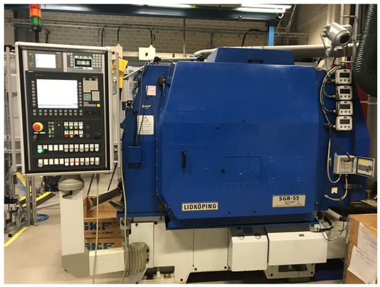
Figure 1.
The Lidköping SGB55 bearing ring grinder used in this investigation.
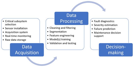
Figure 2.
Implementation steps of CBM process for failure prognostics.
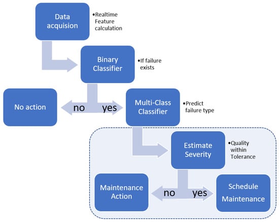
Figure 3.
Failure prediction framework utilizing classification models for failure diagnostics and regression models as severity estimation for the prediction of produced quality. The bounding box represents the scope of this article.
2.1. Data Acquisition
Knowing the maintenance history of the SGB55 grinder, critical subsystems i.e., Grinding Slide assembly and Workhead assembly are monitored with sensors installed on strategic locations [2]. The Figure 4 shows the schematics of the SGB55 grinder and its subsystems. The machine is equipped with sensors, listed in Table 1, for process control as well as additional sensors for condition monitoring. The sensor data is acquired using National Instruments Data Acquisition hardware, cDAQ-9174 with NI-9215 analogue and NI-9423 digital input modules, and the LabView system. The data acquisition system has the capability to simultaneously acquire and store sensor data in sync with the machine’s cyclic operation. For each grinding cycle, the operational parameters are also stored in a database for each grinding cycle.
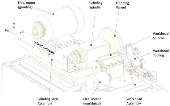
Figure 4.
SGB55’s critical subsystems for sensor installations as part of CBM implementation.

Table 1.
List of sensors installed in SGB55 grinder.
Test and Measurement Criteria
A grinding cycle [28] consisting of a roughing stage and spark-out stage, shown in Figure 5, is programmed to grind the rings. The Roughing stage removes the material to reach the desired dimension of the rings and the Spark-out stage influences the final quality parameters that are being measured at the end. Since the data is acquired w.r.t. the individual grinding cycle, all the ground workpieces for the tests are saved as well. Failure modes are introduced in the selected subsystem components to simulate failures during production. To collect enough statistical data, each test is run for 7 dressing intervals where the grinding wheel is refreshed after each interval. 15 rings are ground in each dressing interval which gives a total of 105 rings for each test and produces 735 rings for all the tests. Figure 6 maps the operating conditions for each type of test and the corresponding rings produced in each test interval. It is infeasible to measure every ring produced using standard equipment. Hence a subset of the produced rings is chosen to be measured for the quality parameters, e.g., form, surface roughness, and waviness, as listed in Table 2. As shown in Figure 6, ring numbers 1, 3, 7, and 15 from each dressing interval are measured for the quality parameters to evaluate the quality being produced during each test run. In addition to the measured quality disparity between different tests, the choice of rings allows capturing the quality variations not only between dressing intervals but also within the dressing interval of a test.
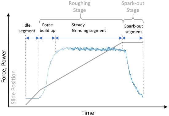
Figure 5.
Grinding cycle to produce parts during tests. The grey line represents the grinding slide position as it moves into the workpiece. Blue represents the resulting in typical force/power signals and the segments that are extracted from each sensor signal for every cycle.
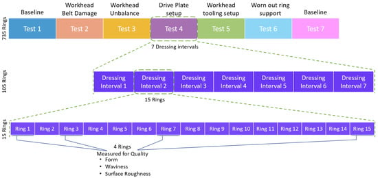
Figure 6.
The figure presents the failure mode tests where the 4, as an example, is expanded to depict the test procedure with dressing intervals and the rings in each of the dressing intervals. This gives a total of 105 rings produced for each test.

Table 2.
Measured Quality Parameters.
2.2. Data Processing
MATLAB® is used for data and signal processing where the data is accessed from the network storage and databases and is cleaned and filtered before further processing [2,27]. Each cycle is divided into segments as shown in the Figure 5 where the Idle segment, the Steady Grinding segment, and the Spark-out segment are isolated from each sensor signal for further processing in feature extraction. To be able to estimate overall ring quality using grinding cycle data, the Spark-out segment is selected for feature engineering. The Table 2 lists the selected main quality parameters derived from quality measurements. Extreme data points resulting from measurement errors can skew the analysis, therefore the quality parameters are cleaned and verified before further processing.
2.2.1. Feature Engineering
After initial data processing, statistical features [26] are extracted from time and frequency domain components of the sensor data for the selected segment. The 9 main quality parameters from measured form, surface roughness, and multiple bands of circumferential waviness are selected as quality features. The quality data is mean normalized per feature for the measured rings according to
where X is the set of observations, is the mean of X and is the standard deviation of X. MATLAB’s Principal Component Analysis (PCA) algorithm is used to calculate principal components through singular value decomposition (SVD).
2.2.2. Sensor Data Feature Set
As part of the failure diagnostics [27], 10 features are extracted from each cycle segment in both time and frequency domain signals. These features are statistical features, namely, mean, standard deviation, skewness, kurtosis, root-mean-square, peak-to-peak, crest factor, band power, energy, and the 90th percentile. Features can be selected based on the segment of interest. As part of feature selection, neighborhood component analysis (NCA) is used due to its computational efficiency and insensitivity towards irrelevant features. The selected features are the top 100 features as per the NCA weight vector that gives minimum classification error [27].
2.2.3. Model Development
To predict the overall quality of the produced parts, the quality predictors need to be trained for quality labels using the sensor data feature set as input. The labeled quality data have to be prepared from multivariate quality measurements. Two approaches are used to prepare labeled data from measured quality parameters. Although serving the same purpose of providing labels the quality predictor model, these approaches provide unsupervised (approach 1) and supervised (approach 2) way of preparing labeled quality data. In each approach, a separate regression learner is trained to predict the overall quality. The quality prediction then can be used to determine if the maintenance action needs triggering.
Approach 1
In the first approach, top 6 principal components are used where the data from 9 quality parameters of measured parts are transformed using the principal component score of the PCA method in MATLAB. The transformed data is then used to perform fuzzy c-means (FCM) clustering, which is an unsupervised clustering approach, using the parameters given in Table 3. The parameters are modified from default values to account for the possible clusters in the quality data with the reduced provision of overlap of the learned clusters. The FCM clustering method allows each data point to belong to multiple clusters with varying degrees of membership. The cluster where the baseline tests, 1 and 7 get higher membership probability is used as the reference cluster for the acceptable quality and a label for the training data set. The regression model is then trained using the sensor signal feature set to estimate the probability of membership of the output quality to the reference cluster.

Table 3.
Optional parameters used for the fuzzy c-means clustering algorithm in MATLAB.
Approach 2
In the second approach, the statistic given by the PCA in MATLAB provides the statistical measure of the multivariate distance of each observation, i.e., ring quality data, from the center of the dataset. The PCA function also supports an output method of Hotelling’s T-Squared Statistic () for the input data according to
where x belong to feature set of observations X, m is the distribution mean of X, is the vector distance of an observation point x from m and is the inverse covariance matrix of X. The PCA method uses all the principal components to compute the T-squared statistic such that it is computed in full feature space. The statistic received for the measured rings becomes the label and is used in training a regression model using the feature set from sensor signal data. The trained model estimates and thus populates a control chart for the ring produced in each grinding cycle given the feature set from the cycle data.
To select the regression learner, MATLAB’s regression learner app is used to train different models ranging from linear and support vector machines to regression trees and random forest. The feature set used to benchmark models originates from the sensor data as mentioned previously in this section. The models are trained separately with quality labels from both approaches including the labels for baseline tests. The random forest regression learner with default hyper-parameters, listed in Table 4, came out to be the top performer in this bench-marking. Hence the random forest regression model is trained further to be the selected overall ring quality estimator.

Table 4.
Hyperparameters used for training of “Fit ensemble of learners for regression” in MATLAB.
2.3. Decision-Making
The significance of any maintenance strategy is reflected through the accuracy and reliability of the maintenance decision-making. The random forest regression learners estimate the overall quality output of individual grinding cycles in terms of predicting the produced quality parameters as a multivariate statistical measure. Failure diagnostic is an important first step which is achieved from random forest classifiers, trained on the feature set from sensor signal data, to predict if the failure exists and the type of failure mode in the acquired data. Once the existing failure mode has been identified, the overall produced quality is predicted.
The random forest regression model from the first approach, trained using data from the FCM clustering method, estimates the probability of the output quality belonging to the reference quality cluster. A pre-selected threshold is used to trigger the maintenance action if the probability falls short of the threshold indicating the failure mode to be severe as the quality reaches the unacceptable limit. This method relies on the accuracy of the learned cluster membership used as a label to train the regression model as well as the selection of the threshold. The FCM clustering, being an unsupervised learning methodology, adds uncertainty to the decision-making as the training of the regression model relies on the learned clusters being representative of the failure and reference classes. The threshold itself adds another dimension that needs optimization based on knowledge and validation through quality measurements.
As for the second approach where the random forest regression model is trained using Hotelling’s T-squared statistic, it estimates the statistic by taking feature set input from sensor data of individual grinding cycles. The statistic can be used to populate the control chart where the quality deviation can also be visually monitored against an upper control limit (UCL). The estimated statistic is compared against the UCL to trigger the maintenance action if the value exceeds the limit. The UCL is calculated based on the data from the baseline tests 1 and 7 according to
where is the confidence level, n is the size of the sample set, k is the size of the subgroup, p is the degrees of freedom and is the F-statistic at . Note that the UCL does not depend on the values calculated for the sample set. Keeping the confidence level less than 100% reduces the chances of false positives in the control chart. This comparison for making the maintenance decision has a dependency on the measurement data itself for the calculation of UCL which acts as the threshold for the predicted quality. Thus it is more reliable and repeatable than the clustering approach where the probability of the learned clusters differing in every iteration is higher. Also, the variation in the incoming data will have a different distribution of quality parameters which will influence the cluster learning significantly.
2.4. Predicted Quality Validation Criteria
The rough grinding considered in this work is the intermediate step in the bearing ring production. Therefore, the produced parts are measured from the tests according to Figure 6. To verify the performance of the proposed model that estimates the overall ring quality, criteria to classify produced rings to be within specifications are defined. Since the multivariate statistic does not signify variations in the individual quality parameters, the entire quality data from the baseline test is taken as a reference. Individual quality parameters for the measured rings are categorized as within specifications if they fall in the of the mean of the parameter of their respective ring number in the baseline test. For a ring to be considered of acceptable quality, at least 4 of the 9 quality parameters are to be within specifications. The pseudo-code for this criteria calculation is presented in the Algorithm 1. This results in the individual quality parameter to be quantified as if within the range and if outside the range. Hence, the rings get classified as either accepted or rejected as per the proposed quality criteria. Thus the ground truth of the measured rings allows the validation of the output of the severity model predictions from the test dataset.
| Algorithm 1 Calculating acceptable quality criteria based on the measured quality parameters. |
|
3. Results and Discussion
This paper is the extension of the previous work where the CBM framework [2] is implemented to achieve intelligent fault diagnosis in the bearing ring grinder [27]. Using information from the implemented CBM setup, to determine the maintenance decision step as per PdM, the quality data is included in the analysis as depicted in Figure 3. As explained in Section 2.1, data from the installed sensors and the machine’s operating parameters are acquired simultaneously for each grinding cycle from which the statistical features are extracted after filtering and segmentation. As described in Section 2.2.2, the top features are chosen based on NCA. Figure 7 shows the heatmap of features extracted from all segments. Since the NCA is insensitive to unnecessary features, a higher weight is given to the best performing features to reach optimum failure classification. The selected feature set for the failure classification results in greater than accuracy, for both the binary and the multi-class failure mode classifier. The intelligent fault diagnosis along with the published dataset [29] and feature and sensor selection for failure mode classification are covered in the implementation of the CBM setup for the bearing ring grinder [27].
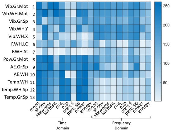
Figure 7.
Heatmap of features from all segments as per NCA weights. A higher value indicates a higher feature ranking. Here Vib = Vibration, Gr = Grinding, Mot = Motor, WH = Workhead tooling, Sp = Spindle, F = Force, LC = Load Cell, St = Strain gauge, Pow = Electric Power, AE = Acoustic Emission, Temp = Temperature. Adapted from [27].
The produced rings from the experimental test runs are measured as described in the Section 2.1. The Figure 8 shows the box plot of surface roughness and circumferential form measurement of all the measured rings. It is to be noted that different types of failure modes will affect the measured parameters differently as evident for the two quality parameters, surface roughness (Ra) and form, as shown in the Figure 8. The PCA from the 9 measured quality parameters of the produced parts is shown in Figure 9. Although more than of the variance is explained by the first two principal components, it is not enough to separate all the test classes. From the Figure 9, the tests 1, 2, 3, and 7 seem to overlap. Since tests 1 and 7 are reference baseline tests, they are bound to be closer to each other in the hyperspace. Due to less severity of the failure modes 2 and 3, statistically, it is possible to produce parts within tolerance. At this early stage of material removal in production, it will not be possible to identify quality variations resulting from these failure modes due to the limited number of in-line quality parameters being measured.
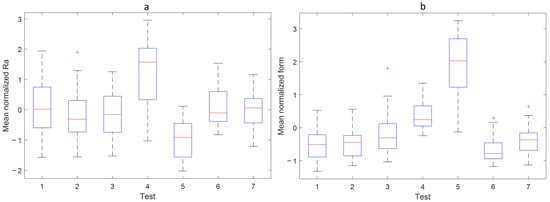
Figure 8.
Box plot of (a) Mean Normalized Surface Roughness and (b) circumferential form measurement. The box plot for each test 1–7 includes measured rings from all the dress cycles. The red + indicate outlier value that is more than times interquartile range away from bottom or top of the box.
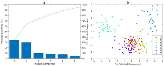
Figure 9.
The Pareto plot in subfigure (a) shows more than of the variance explained by 6 principal components. The scatter plot in subfigure (b) for the first two principal components shows the separation of the test classes 1–7 as per Figure 6.
As explained in Section 2.2.3 for the Approach 1 using the fuzzy c-means clustering algorithm, the top 6 principal components are used to learn 4 quality clusters in MATLAB using the parameters listed in the Table 3. The 4 number of clusters better explained the variations before the clusters within a class start to appear. Examining the raw quality data from a domain expert perspective also suggests the close existence of the test classes as shown in Figure 9. The learned cluster centers from the FCM clustering algorithm, in Figure 10, are presented in the first 2 principal component dimensions. The resulting allocation of each test class for the 4 centers is depicted in a stacked bar plot in the Figure 11. Since FCM is based on optimization, the cluster allocation varies for each run of the algorithm which affects the repeatability of the results in this approach. From the Figure 11, it is evident that the cluster center 4 is the reference cluster and is used as the quality label to train the regression model.
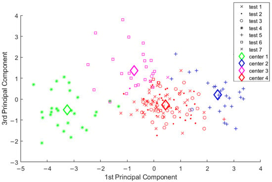
Figure 10.
Clusters and cluster centers visualized in the plane of the two principal components.
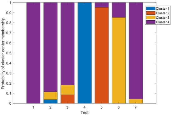
Figure 11.
Probability or degree of cluster center membership to the individual quality observation of the respective test classes in 6 PCA dimensions.
The selected regression model is the random forest as per MATLAB’s regression learner app benchmark figures presented in the Table 5. Thus the center 4 data, representing the degree of membership for each measured observation, is used as a label to train the random forest regression model with an achieved Root Mean Square Error (RMSE) of out of the max scale of 1. The low RMSE gives a good predictor which is evident from the Figure 12 where the test data from tests 1 and 7 are estimated to be belonging to the reference cluster. The uncertainty in cluster learning and cluster center membership allocation makes it difficult to repeatedly use the method for reliable predictability. The significant difference between the benchmark and the presented first approach’s RMSE results from FCM-based labeled data is evidence of the inherent fuzzy behavior of the algorithm directly influencing the performance accuracy.

Table 5.
Bench-marking of regression models in MATLAB’s regression learner app. Quality Label columns represent the achieved Root Mean Square Error (RMSE) for the labels used from the two approaches in training the models.
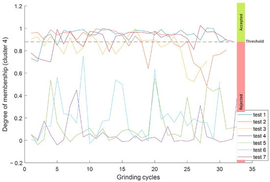
Figure 12.
Predicting the overall ring quality produced in test data. The dashed line represents the threshold above which the quality is acceptable.
In contrast, the Approach 2 of Hotelling’s T-squared statistic is less uncertain due to repeatability and reliability based on the available data. The statistic values achieved from the output of the PCA algorithm in MATLAB are used as labels to train the random forest regression learner using default hyper-parameters and only modifying the ones listed in the Table 4. The training of the regression learner results in an RMSE of out of max scale value of which, in terms of error rate, is lower than the RMSE of Approach 1, i.e., . The UCL calculated from the training quality dataset using the Equation (3) becomes with the confidence level of obtained from . The training dataset when compared against the UCL is shown in Figure 13.
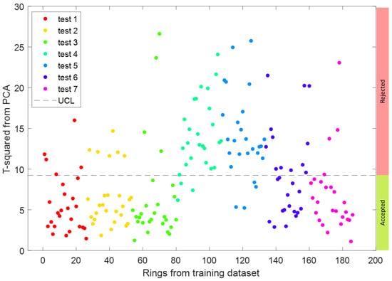
Figure 13.
Calculated statistic from training quality dataset using MATLAB’s Principal Component Analysis (PCA) algorithm. The dashed line represents Upper Control Limit (UCL).
The regression model estimations on the test set of sensor feature set are shown in the Figure 14. The UCL is shown as a dashed line and serves as a threshold above which the quality becomes unacceptable. Even though the test set, comprising of feature set from the selected segment of the sensor data, is larger than the entire quality dataset, the results follow the trend of the training set of measured quality. It is only fitting to verify the regression model predictions using absolute truth which is the measured ring quality itself. The box plot in the Figure 15 depicts the classification of measured rings as accepted or rejected based on the criteria defined in Section 2.4. The threshold is the limit representing 4 out of 9 measured quality parameters to be within the accepted tolerance limit. The overall quality scale in the Figure 15 is the average of quality parameters disposition where a higher level means more quality parameters out of specifications. Note that the criteria result in the classification of individual rings based on all the measured quality parameters. Hence, the measured rings that end up out of spec according to quality criteria are represented as red circle markers in the Figure 14. Most of the markers being above the UCL line of the plot verify the performance of the model on the test set with calculated accuracy of more than on the corresponding rings measured for quality. In comparison, the FCM approach has less absolute differentiation between the quality data from different test classes which confirms the overlapping quality clusters in the hyper-space. However, the results from the statistic are repeatable which is desirable in any failure prediction model.
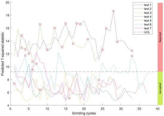
Figure 14.
Predicting the overall produced quality in test data through estimating statistic. The dashed line represents Upper Control Limit threshold above which the quality is unacceptable. The red circle markers indicate the rejected rings according to quality criteria.
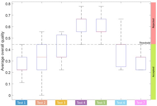
Figure 15.
Box plot showing the quantification of the quality produced in each test after the acceptance criteria have been applied to the measured parts.
The results presented here demonstrate the potential of using data from the sensors, e.g., acoustic emission, vibration, force, power, and temperature, installed for the purpose of process control and condition monitoring to predict quality in a bearing ring grinder. In this work, the class balance has been ensured in setting up the experimental tests to avoid over-representation of any failure mode in the dataset [2]. Although different failure modes affect the measured quality parameters differently, the defined quality criteria account for the individual parameter in comparison to the reference quality test. The high accuracy prediction results achieved on the dataset give the confidence to use the presented approach in regular production to estimate overall quality for rings using the sensor data only.
4. Conclusions
This paper presents an approach to predicting the overall quality of ground bearing rings using a feature set from the sensor data. The grinder is equipped with additional acoustic emission, vibration, force (strain), and temperature sensors for machine health monitoring purposes. The feature set, resulting from the failure diagnostics using sensor data, is also used to benchmark the random forest as a top-performing regression model to estimate the quality of the produced rings. Using Hotelling’s T-squared statistic to generate quality labels is presented as the preferred choice over fuzzy c-means clustering, for its repeatable results. The model prediction is compared against a threshold value for ring quality disposition to trigger a maintenance action. The quality criteria based on individual quality parameters validate the proposed model performance with accuracy on the test set of measured rings. The use of multivariate quality statistic ensures the consideration of all quality parameter variations that are otherwise infeasible to measure in-line during the grinding operation. Thus, this work successfully demonstrates the possibility to use the data from the installed sensors to not only estimate the condition and performance but also to predict the produced quality variations of the production grinder. The high accuracy achieved in predicting the overall quality evidently shows the effectiveness of such decision support in triggering maintenance action. The potential to improve performance through enhanced quality classification criteria needs to be verified through extended testing and measurement of the produced parts. Additionally, individual quality parameters can be predicted to take specific remedial actions. However, for the scope of this work, the herein presented approach demonstrates an efficient and effective implementation of a maintenance decision support system for a bearing ring grinder. With the availability of multiple sensor data from the entire grinding cycle, using more sophisticated data processing and model development can be considered to improve failure prognostics as part of predictive maintenance.
Author Contributions
All authors contributed to the study’s conception and design. Instrumentation, software, testing, formal analysis, and data curation were performed by M.A. Data collection and analysis was supervised by F.S., P.M. and M.G. and reviewed by F.S., P.M., M.G. and K.B. The first draft of the manuscript was written by M.A. and all authors commented on previous versions of the manuscript. All authors have read and agreed to the published version of the manuscript.
Funding
This research received no external funding.
Institutional Review Board Statement
Not applicable.
Informed Consent Statement
Not applicable.
Data Availability Statement
The dataset will be made available along with the acceptance and publication of this manuscript (URN: http://urn.kb.se/resolve?urn=urn:nbn:se:ltu:diva-92569, accessed: 7 September 2022).
Conflicts of Interest
The authors declare no conflict of interest.
References
- Urgoiti, L.; Barrenetxea, D.; Sánchez, J.A.; Godino, L. Experimental study of thermal behaviour of face grinding with alumina angular wheels considering the effect of wheel wear. CIRP J. Manuf. Sci. Technol. 2021, 35, 691–700. [Google Scholar] [CrossRef]
- Ahmer, M.; Marklund, P.; Gustafsson, M.; Berglund, K. An implementation framework for condition-based maintenance in a bearing ring grinder. Procedia CIRP 2022, 107, 746–751. [Google Scholar] [CrossRef]
- Tönshoff, H.; Friemuth, T.; Becker, J. Process Monitoring in Grinding. CIRP Ann. 2002, 51, 551–571. [Google Scholar] [CrossRef]
- Teti, R.; Jemielniak, K.; O’Donnell, G.; Dornfeld, D. Advanced monitoring of machining operations. CIRP Ann. 2010, 59, 717–739. [Google Scholar] [CrossRef]
- Wegener, K.; Bleicher, F.; Krajnik, P.; Hoffmeister, H.W.; Brecher, C. Recent developments in grinding machines. CIRP Ann. 2017, 66, 779–802. [Google Scholar] [CrossRef]
- Fedele, L. Methodologies and Techniques for Advanced Maintenance; Springer: London, UK, 2011. [Google Scholar] [CrossRef]
- Diez-Olivan, A.; Del Ser, J.; Galar, D.; Sierra, B. Data fusion and machine learning for industrial prognosis: Trends and perspectives towards Industry 4.0. Inf. Fusion 2019, 50, 92–111. [Google Scholar] [CrossRef]
- Zhang, P.; Gao, Z.; Cao, L.; Dong, F.; Zou, Y.; Wang, K.; Zhang, Y.; Sun, P. Marine Systems and Equipment Prognostics and Health Management: A Systematic Review from Health Condition Monitoring to Maintenance Strategy. Machines 2022, 10, 72. [Google Scholar] [CrossRef]
- Teixeira, H.N.; Lopes, I.; Braga, A.C. Condition-based maintenance implementation: A literature review. Procedia Manuf. 2020, 51, 228–235. [Google Scholar] [CrossRef]
- Heng, A.; Zhang, S.; Tan, A.C.; Mathew, J. Rotating machinery prognostics: State of the art, challenges and opportunities. Mech. Syst. Signal Process. 2009, 23, 724–739. [Google Scholar] [CrossRef]
- Goyal, D.; Pabla, B. Condition based maintenance of machine tools—A review. CIRP J. Manuf. Sci. Technol. 2015, 10, 24–35. [Google Scholar] [CrossRef]
- Jardine, A.K.; Lin, D.; Banjevic, D. A review on machinery diagnostics and prognostics implementing condition-based maintenance. Mech. Syst. Signal Process. 2006, 20, 1483–1510. [Google Scholar] [CrossRef]
- Camci, F. Process monitoring, diagnostics and prognostics using support vector machines and hidden Markov models. Ph.D. Thesis, Wayne State University, Detroit, MI, USA, 2005. [Google Scholar]
- Dragomir, O.E.; Gouriveau, R.; Dragomir, F.; Minca, E.; Zerhouni, N. Review of prognostic problem in condition-based maintenance. In Proceedings of the 2009 European Control Conference (ECC), Budapest, Hungary, 23–26 August 2009; pp. 1587–1592. [Google Scholar] [CrossRef]
- Leukel, J.; González, J.; Riekert, M. Adoption of machine learning technology for failure prediction in industrial maintenance: A systematic review. J. Manuf. Syst. 2021, 61, 87–96. [Google Scholar] [CrossRef]
- Lei, Y.; Yang, B.; Jiang, X.; Jia, F.; Li, N.; Nandi, A.K. Applications of machine learning to machine fault diagnosis: A review and roadmap. Mech. Syst. Signal Process. 2020, 138, 106587. [Google Scholar] [CrossRef]
- Orth, P.; Yacout, S.; Adjengue, L. Accuracy and robustness of decision making techniques in condition based maintenance. J. Intell. Manuf. 2009, 23, 255–264. [Google Scholar] [CrossRef]
- Vollert, S.; Atzmueller, M.; Theissler, A. Interpretable Machine Learning: A brief survey from the predictive maintenance perspective. In Proceedings of the 2021 26th IEEE International Conference on Emerging Technologies and Factory Automation (ETFA), Vasteras, Sweden, 7–10 September 2021. [Google Scholar] [CrossRef]
- Amruthnath, N.; Gupta, T. Fault Diagnosis Using Clustering. What Statistical Test to use for Hypothesis Testing? Mach. Learn. Appl. Int. J. 2019, 6, 17–33. [Google Scholar] [CrossRef]
- AlGhazzawi, A.; Lennox, B. Monitoring a complex refining process using multivariate statistics. Control Eng. Pract. 2008, 16, 294–307. [Google Scholar] [CrossRef]
- Salehi, M.; Bahreininejad, A.; Nakhai, I. On-line analysis of out-of-control signals in multivariate manufacturing processes using a hybrid learning-based model. Neurocomputing 2011, 74, 2083–2095. [Google Scholar] [CrossRef]
- Peng, Y.; Dong, M.; Zuo, M.J. Current status of machine prognostics in condition-based maintenance: A review. Int. J. Adv. Manuf. Technol. 2010, 50, 297–313. [Google Scholar] [CrossRef]
- Carvalho, T.P.; Soares, F.A.A.M.N.; Vita, R.; da P. Francisco, R.; Basto, J.P.; Alcalá, S.G.S. A systematic literature review of machine learning methods applied to predictive maintenance. Comput. Ind. Eng. 2019, 137, 106024. [Google Scholar] [CrossRef]
- Schwendemann, S.; Amjad, Z.; Sikora, A. A survey of machine-learning techniques for condition monitoring and predictive maintenance of bearings in grinding machines. Comput. Ind. 2021, 125, 103380. [Google Scholar] [CrossRef]
- Tsui, K.L.; Chen, N.; Zhou, Q.; Hai, Y.; Wang, W. Prognostics and Health Management: A Review on Data Driven Approaches. Math. Probl. Eng. 2015, 2015, 793161. [Google Scholar] [CrossRef]
- Ahmer, M.; Marklund, P.; Gustafsson, M.; Berglund, K. Integration of process monitoring and machine condition diagnostics to improve quality prediction in grinding. Procedia CIRP 2021, 101, 170–173. [Google Scholar] [CrossRef]
- Ahmer, M.; Sandin, F.; Marklund, P.; Gustafsson, M.; Berglund, K. Failure mode classification for condition-based maintenance in a bearing ring grinding machine. Int. J. Adv. Manuf. Technol. 2022; in press. [Google Scholar] [CrossRef]
- Shore, P.; Billing, O.; Puhasmagi, V. A Standard Grinding Wheel Assessment Method to Support a Sophisticated Grinding Knowledge Based System. Key Eng. Mater. 2004, 257–258, 285–290. [Google Scholar] [CrossRef]
- Ahmer, M.; Sandin, F.; Marklund, P.; Gustafsson, M.; Berglund, K. Dataset Concerning the Process Monitoring and Condition Monitoring Data of a Bearing Ring Grinder; Luleå University of Technology: Lule, Sweden, 2022. [Google Scholar] [CrossRef]
Publisher’s Note: MDPI stays neutral with regard to jurisdictional claims in published maps and institutional affiliations. |
© 2022 by the authors. Licensee MDPI, Basel, Switzerland. This article is an open access article distributed under the terms and conditions of the Creative Commons Attribution (CC BY) license (https://creativecommons.org/licenses/by/4.0/).