Article

A Study on Gear Defect Detection via Frequency Analysis Based on DNN

1
Electrical and Electronic Convergence Department, Hongik University, Sejong 30016, Korea
2
Electronic and Electrical Department, Sungkyunkwan University, Suwon 03063, Korea
*
Author to whom correspondence should be addressed.
Machines 2022, 10(8), 659; https://doi.org/10.3390/machines10080659
Submission received: 12 July 2022 / Revised: 2 August 2022 / Accepted: 3 August 2022 / Published: 5 August 2022
(This article belongs to the Section Robotics, Mechatronics and Intelligent Machines)

Abstract

:
In this paper, we introduce a gear defect detection system using frequency analysis based on deep learning. The existing defect diagnosis systems using acoustic analysis use spectrogram, scalogram, and MFCC (Mel-Frequency Cepstral Coefficient) images as inputs to the convolutional neural network (CNN) model to diagnose defects. However, using visualized acoustic data as input to the CNN models requires a lot of computation time. Although computing power has improved, there is a situation in which a processor with low performance is used for reasons such as cost-effectiveness. In this paper, only the sums of frequency bands are used as input to the deep neural network (DNN) model to diagnose the gear fault. This system diagnoses the defects using only a few specific frequency bands, so it ignores unnecessary data and does not require high performance when diagnosing defects because it uses a relatively simple deep learning model for classification. We evaluate the performance of the proposed system through experiments and verify that real-time diagnosis of gears is possible compared to the CNN model. The result showed 95.5% accuracy for 1000 test data, and it took 18.48 ms, so that verified the capability of real-time diagnosis in a low-spec environment. The proposed system is expected to be effectively used to diagnose defects in various sound-based facilities at a low cost.

1. Introduction

Since the advent of the third industrial revolution, automation of various manufacturing plants has been achieved [1,2,3]. An automated system refers to a system that does not require manpower but uses equipment such as computers and robots to operating the entire process [4]. Smart factory is an intelligent factory that can efficiently produce products by integrating elements from the entire process, such as planning, design, production, distribution, and sales, into Cyber Physical System (CPS), Internet of Things (IoT), robot, 3D printing, and big data [5]. Automation plants have been applied to many industrial sites because of their potential to improve productivity and reduce labor costs. Therefore, smart factories have been highlighted and studied intensively [6,7].
Automation machines can reliably increase production, but when defects or failures occur, it is difficult to find out the cause of the problem due to the complex production process and system [8]. This is especially true when one has to go through a complicated process of disassembling and inspecting equipment, such as piping and assembled machines [9]. Real-time fault diagnosis of automated machines is an important technology that can prevent both economic and human damage/loss. Although periodic failure inspections of such automation equipment are required for stable operation of the automation process, there is the problem that the inspection requires a lot of manpower and cost.
Acoustic analysis refers to analyzing sound signals collected through sensors such as microphones. Acoustic analysis is widely used in that it is possible to obtain target data without dismantling the target using inexpensive sensors [10,11]. The analysis of acoustic signals identifies time, amplitude, and frequency components, and identifies interesting characteristics by applying various techniques according to the purpose. Above all, frequency analysis of acoustic signals makes it easy to analyze the periodicity of signals and filter noisy signals. It is also widely used in the analysis of acoustic signals because it can extract frequency characteristics of specific signals well [12], and spectrograms [13], scalograms [14], and mel-frequency cepstrum coefficient (MFCC) [15] are graphs that show changes in frequency intensity over time by converting acoustic signals into time-frequency axes. Each of these time-frequency image-based methods is specialized in analyzing a frequency change pattern over time or a change in a dominant frequency range of an acoustic signal.
Frequency analysis of acoustic signals is widely used to detect various defects, such as determining the degree of wear of the machine or detecting defects in bearings. Before deep learning was studied intensively, numerical, analytical, and experimental research was performed [16,17,18]. After application of artificial intelligence became active, various studies to detect mechanical fault based on deep learning were introduced. Research has been conducted to diagnose gear failures using vibration signals based on fuzzy neural networks [19]. Research has been conducted on a mechanical defect diagnostic convolutional neural network (CNN) model that uses acoustic signals as input to make them robust to the changing sound of the domain [20,21]. Research has been conducted to visually detect defects in gears using image-based, region-based convolutional neural networks (R-CNN) [22]. Studies have been conducted to diagnose failure of gear fitting using both vibration and sound emission signals using CNN and gated recurrent unit (GRU) [23]. A spectrogram ball-and-roller bearing with the image was used to diagnose defects in a study relating to the model CNN [24]. When diagnosing defects in rolling bearings, studies were conducted comparing the performance of spectrogram, scalogram, and Hilbert sulfur images [25]. Based on the CNN model, a study on the failure diagnosis technique of the automated machine using spectrogram images was conducted [26]. Based on unsupervised learning, a study was conducted to detect the failure using spectrogram images [27]. Another study was conducted to diagnose the failure by using spectrogram images of acoustic data filtering ambient noise as input to neural network models [28], and yet another was conducted on the fault diagnosis and analysis of transition learning-based facilities using spectrogram images [29]. The advantage of using a spectrogram image to diagnose defects in a machine is that it is possible to check the frequency change over time, so it is possible to make a more accurate diagnosis. However, there is a disadvantage in that the process of converting sound signals into spectrogram images is added, and images are used as input to artificial neural networks, which increases the computation volume and requires high performance, making real-time diagnosis difficult. Although computing power has increased rapidly, there are situations in which low-performance hardware is used for cost-effectiveness issues.
In this paper, the spectral data of recorded sounds are used as input for deep learning models to diagnose defects in gears. Raw spectral data are not suitable for real-time monitoring due to a large amount of computation to use all spectral data as input due to various frequency ranges. Therefore, the sums of frequency bands that represent the characteristics of rotating gears are used as an input to the deep neural network (DNN) model. By selecting frequency bands, it is also available to detect faults for several different gear RPMs. We note that such works are already shown in bearings [30]. The model is trained in advance by collecting the acoustic signal of rotating gears by type. For defect diagnosis, the sound of the rotating gear is converted into spectral data and the sum of the frequency bands is calculated to be used as an input to a pre-trained deep-learning-based classifier model to determine the current state [31].

2. Materials and Methods

In this paper, acoustic data are analyzed in the frequency domain and used as input to a pre-trained deep learning model to diagnose gear defects. Figure 1a shows the setting of this system and Figure 1b shows the types of gear states pre-trained for the classification of defect types. From the top left to the bottom right, there are four types in order: ‘normal’, ‘one tooth broken’, ‘four teeth broken’, and ‘all worn out’.
Figure 2 shows the schematic diagram of operating the system proposed in this paper. The acoustic data of the gear are converted into a frequency domain through Fast Fourier Transform (FFT). After that, the amplitude of the preset frequency band of interest is summed respectively to use as a feature for diagnosing the type of defect. The feature is used as an input to a pre-trained deep learning model to output the type of defect diagnosis of the gear.

2.1. Sound Data Collection for Acoustic Analysis

Sound data are collected in real time using a microphone to diagnose the gear defect of the system. In order to collect gear sound data, we install a microphone in the center of the rotating gear. We used a condenser microphone to collect sound data. The condenser microphone has the advantage of sensitivity and a wide range of polar patterns compared to the dynamic microphone. The condenser microphone has a high risk of howling caused by the sound of other surrounding speakers, but we used a condenser microphone because the howling was less likely to occur in the environment of this paper [32]. The condenser microphone used in this paper has a 100~16,000 Hz frequency band and −47 dB ± 4 sensitivity.
We used ‘pyaudio’ [33] library for sound data collection and a 44,100 Hz sampling rate. Since the maximum frequency of sound data that can be sampled according to the Nyquist theorem is 22,050 Hz, it can collect the gear sound of the 7000 Hz band generated in this paper [34]. The collected data are used to diagnose the gear defect in real time through deep-learning-based spectrum analysis.

2.2. Sound Data Pre-Processing

If we apply sound data without pre-processing in an artificial intelligence model for diagnosing gear defects, the size of the input data increases unnecessarily and the amount of computation increases, resulting in an increase in processing time. In addition, through pre-processing, the train data increase, and better performance can be expected. Therefore, the feature extraction through acoustic spectrum analysis is performed so that the features of each defect type are prominent. We also use data augmentation to increase train data and improve robustness from external factors [35].

2.2.1. Data Augmentation

One of the representative methods used in artificial intelligence models to improve robustness from external factors such as noise and distortion is data augmentation [36]. Data augmentation transforms existing data to increase the amount of data and uses it as train data. Data augmentation can improve the performance of artificial intelligence models by increasing the amount of train data, and appropriate methods are selected and used according to the type and characteristics of the data.
Techniques for sound data augmentation include volume control, stretching, white noise, flip, reverb, and overlap. In this paper, volume control and stretching methods with changing amplitudes and frequency components are not suitable because the state is diagnosed using the sum of amplitudes in a specific frequency band by collecting gear sounds and spectral analysis of sound data. Therefore, in this paper, we used white noise, flip, reverb, and overlap methods for data augmentation.
For white noise, we added a random signal with 1/20 of the maximum amplitude of the signal. Adding white noise makes the system tough from ambient noise. In terms of flip, the graph was flipped by inversing the raw data. This simple method provides more information to the model because the flipped data also still contain acoustic information. As for the reverb, we used ‘reverb’ in the ‘Pedal Board’ [37] library and set the room size to 0.25. This method augments the data by adding reverberations so that the model is robust against the environment in which reverberations occur. For overlap, when slicing the raw data, the overlapping part was set to 0.44 s. Overlap is a widely used data augmentation method to augment a small amount of sound data.

2.2.2. Acoustic Spectral Analysis

Sound data collected through the microphone must be extracted for each type of feature through spectral analysis for the train and classification of artificial intelligence models. Figure 3 shows a flowchart of sound spectrum analysis for classification model training. First, the collected sound data are converted into spectral data through Fourier transform, and then the frequency domain of interest is extracted according to the gear noise characteristics of the system. The number of gear teeth used in this paper is 16, operating at RPMs of 140, 280, and 420 [38]. We selected three RPMs, since in a real system several different gears or gear RPMs will be used simultaneously. We checked the spectrum of the four types of gears for the corresponding frequency bands, and set the frequency bands such that each type can be distinguished as the frequency domain of interest. After that, the sum of the amplitudes of each section of the frequency domain of interest is calculated. The sum of the amplitudes of each frequency section calculated in this way has a different distribution for each type and is used as the train and input data to be used in artificial intelligence models.
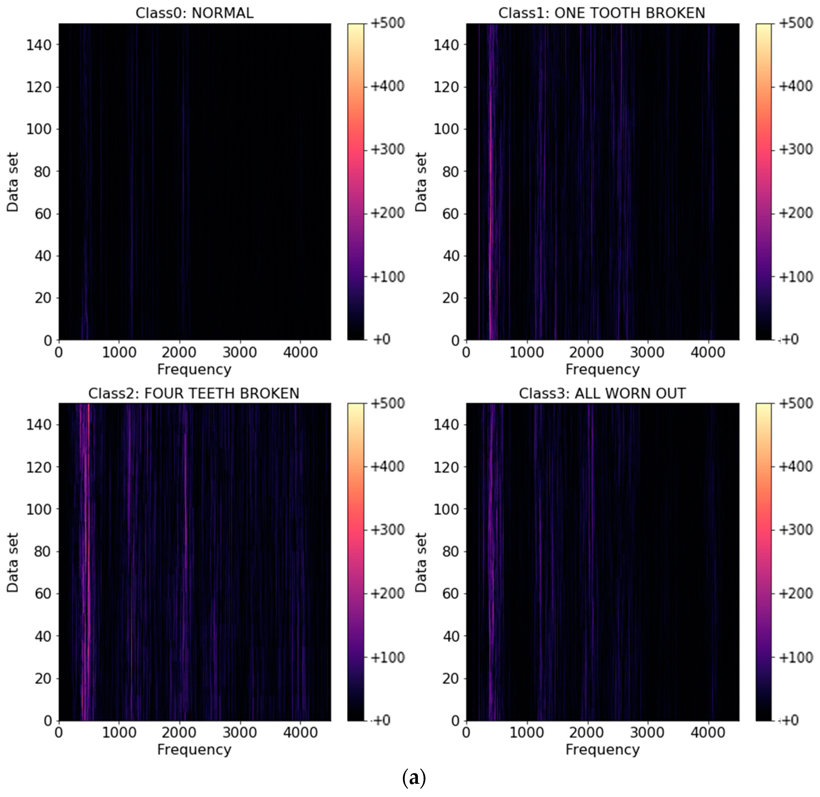
The collected sound data of time series are converted into the frequency domain using Fourier transform for spectral analysis. For low computation and high speed, FFT was used for Fourier transform. For FFT, we used the ‘fft’ function of the ‘numpy’ library [39]. Note that fft is adopted because the Descrete Fourier Transform (DFT) algorithm is difficult to use in low-spec hardware specifications. According to the Nyquist theorem, since the sampling rate is 44,100 Hz, the frequency band of the sound data is 0 to 22,050 Hz. Figure 4a shows 150 samples of acoustic data in terms of frequency for each case.
To minimize the input size, we have integrated the spectrums in a few regions. The equation is shown as follows:
F n = f s t a r t , n f e n d , n S   df ,
where Fn is the nth input and fstart,n and fend,n constitute the nth range of interest.
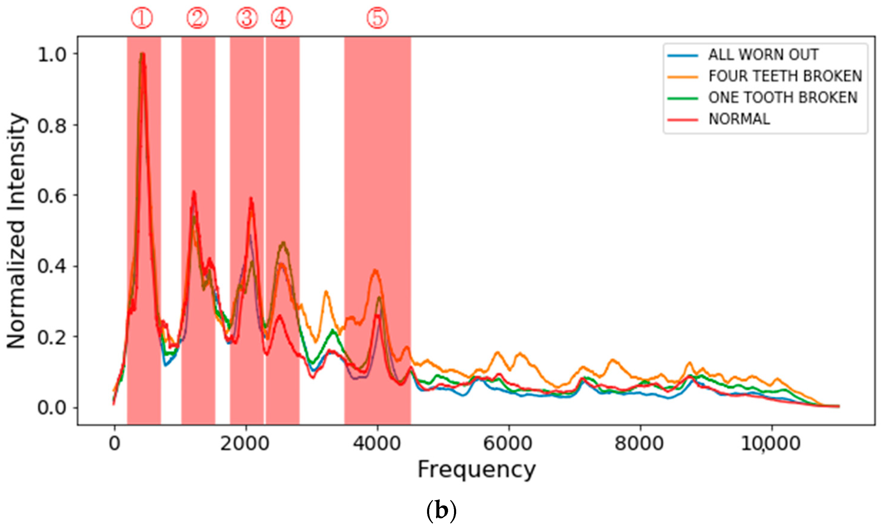
Figure 4b shows averaged spectrum of the sound data. We used the frequency band corresponding to the peak in the spectrum graph for the analysis. The figure shows an example of frequency band selection. In this case, five bands are chosen to be the band of interest, which are 200~700 Hz, 1000~1500 Hz, 1700~2200 Hz, 2200~2700 Hz, and 3500~4500 Hz. In other words, n is 5 and fstart,n is 200 Hz, fend,1 is 700 Hz. We summed the amplitude of each frequency band and used it as the feature for each defect type. When the gear is defective, the characteristics of the noise will be different, and the ratio of each sum of frequency amplitude will be also different, so we can use this difference as the feature of each defect type. These features can be used as train data for classifiers based on deep learning.
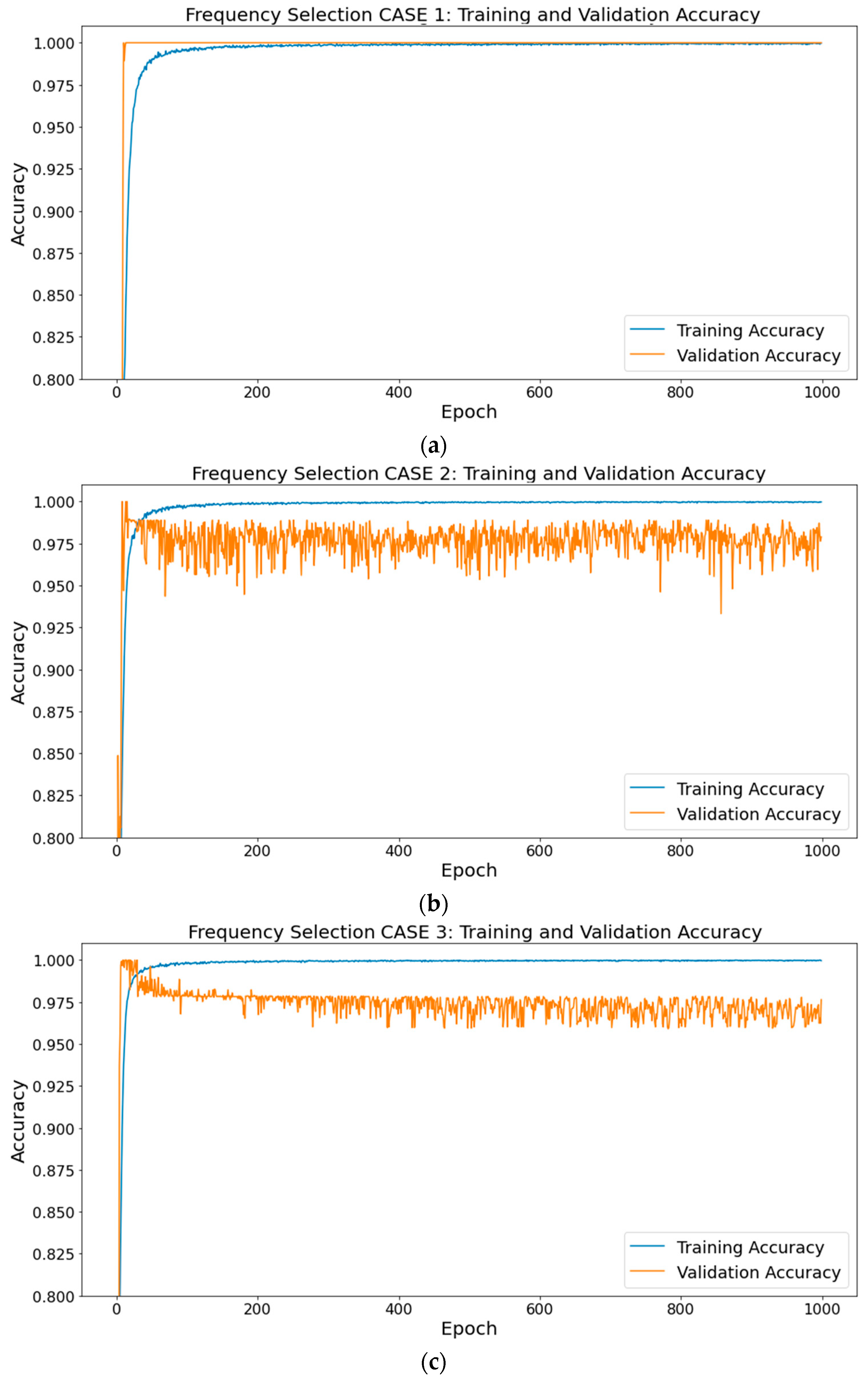
Various peaks are observed in Figure 4b. To select the range and region of interest for the model input, we have checked three cases of frequency selection. Table 1 shows the region of the three selection cases. Note that the frequency band of the region has been selected to cover the full-width half-max (FWHM) of each peak. We have trained the model by using these three cases, and the training accuracy in terms of epochs is shown in Figure 5. It is clear that case 2 and case 3 show low accuracy, and the loss oscillates. Therefore, we select the band of interest as the frequency selection case 1 in Table 1. As shown in these results, some wrong selection of frequency band is unavailable to distinguish the fault correctly. However, as some noises are frequency-independent, but some of the noises form a band [40], correct selection of frequency band is proper to detect noise.

2.3. Train Dataset

We used the sum of each frequency band of interest amplitude as the train dataset for the classifier based on deep learning through sound data augmentation and acoustic spectral analysis. Sound data used for the train were collected at a sampling rate of 44,100 Hz, and sound data with a length of 1 s were converted into a frequency domain through FFT. The dataset contains four classes: ‘normal’, ‘one tooth broken’, ‘four teeth broken’, and ‘all worn out’. In terms of the dataset, a total of 14,486 data were used, with 10,775 train data, 2707 validation data, and 1000 test data. The datasets are divided randomly.
The sum of the amplitude of each frequency band is data with a very large deviation in value. When training the model, if the deviation of the train data is large, the train weights are likely to be overfitting. Therefore, train data are normalized to suppress overfitting of weights [41]. In this paper, we used MinMaxScaler of ‘sklearn’ library for normalizing data, which normalized the data between 0 to 1 [42].

2.4. Training

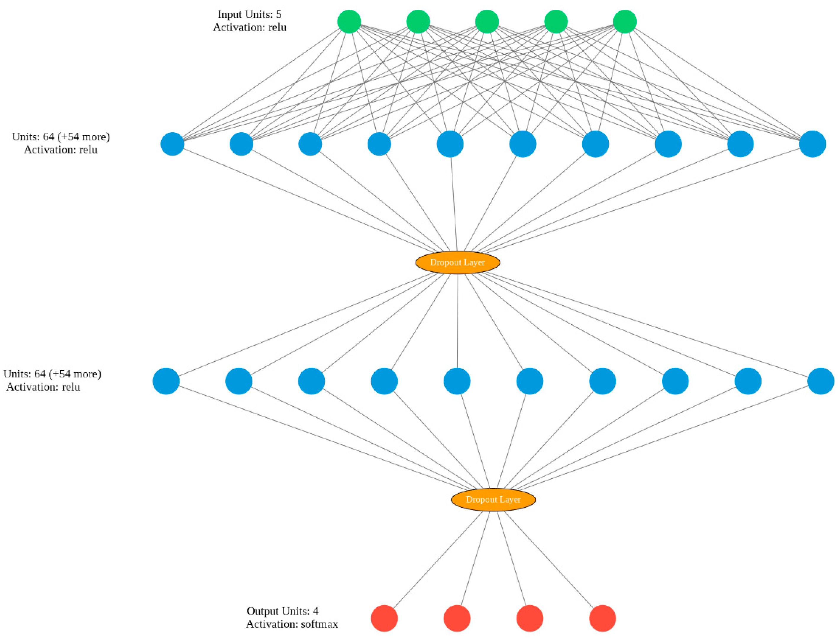
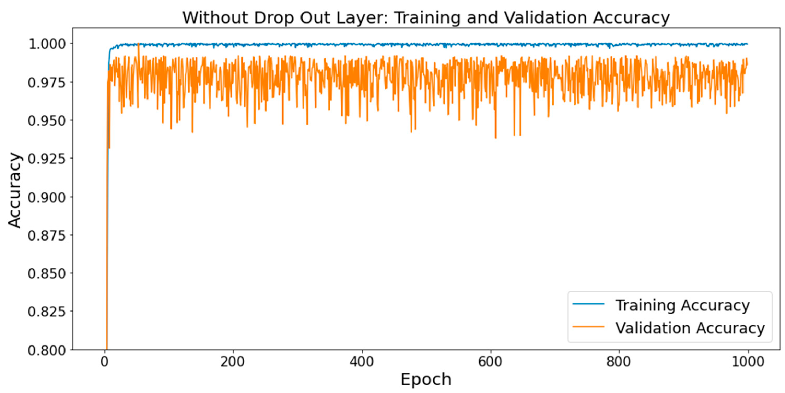
Table 2 and Figure 6 show DNN model architecture for defect diagnosis in this paper. The model architecture used in this paper includes three dense layers and two dropout layers, as well as a classifier for classification. The dropout layer is applied to reduce overfitting. Without the dropout layer, the model showed 96.44% accuracy on validation and test datasets as shown in Figure 7. It is shown that the accuracy of the validation set does not converge without the dropout layer. It is also notable that the hyper-parameters such as node number and number of hidden layers are optimized.
The inputs use a total of five inputs as the sum of the amplitudes of each section in the frequency band of 200~4500 Hz. There are four types of output as the classification result: ‘0: normal’, ‘1: one tooth broken’, ‘2: four teeth broken’, and ‘3: all worn out’. Therefore, as shown in Figure 6, the model has 5 inputs and 4 outputs.
Dropout was added between each layer to prevent overfitting of the train data. As an activation function of Classifier, Softmax is used to output the accuracy of each class so that multiple classes can be classified.
To train the model, 14,486 datasets were trained 1000 times with a batch size of 32, using the previous DNN architecture. In this paper, we used the model with the highest accuracy in the training process after 1000 times of train. Stochastic Gradient Descent (SGD) was used as an optimizer, and Categorical Cross Entropy (CCE) was used for loss function calculation.
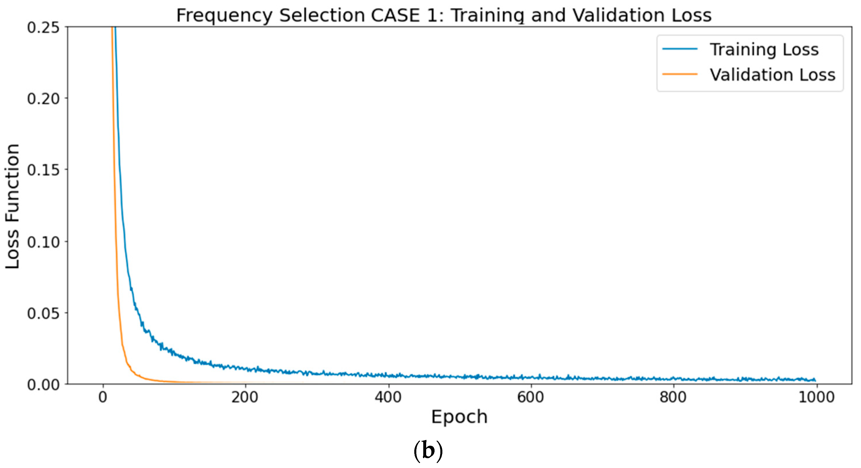
Figure 8 shows the accuracy and loss of training sets and validation sets during the training process. The figure shows the loss is well converged with an accuracy of 99.97% and a loss of 0.0015. Even with a small number of trains, it shows high accuracy.
To verify the robustness of our model, we used K-Fold cross validation to test the strength of the model. The K value was chosen to be 5 and the training-validation set was divided into five sections, one of which was used as a validation set. The accuracy was 99.97%, 95.78%, 98.09%, 96.52% and 99.61%, respectively, with an average of 97.99%, which confirms the robustness of our model.

3. Experiment and Results

3.1. Experiment Environment

In the experiment, we used the noise of working gear, and the calculation was performed using a laptop computer without an external GPU to verify the efficiency and compactness of the proposed system.
In the experiment, sound data when various defect types of gears operate were used. In order to verify efficiency, for the hardware specifications we experimented with a low-power CPU for laptops without an external GPU, which are shown in Table 3.
Experiments were carried out with gear sound that was never used for train and validation, and various defect types were used. A total of 1000 test data were used for the experiment with 250 data for each type.

3.2. Result of Experiment with Test Dataset

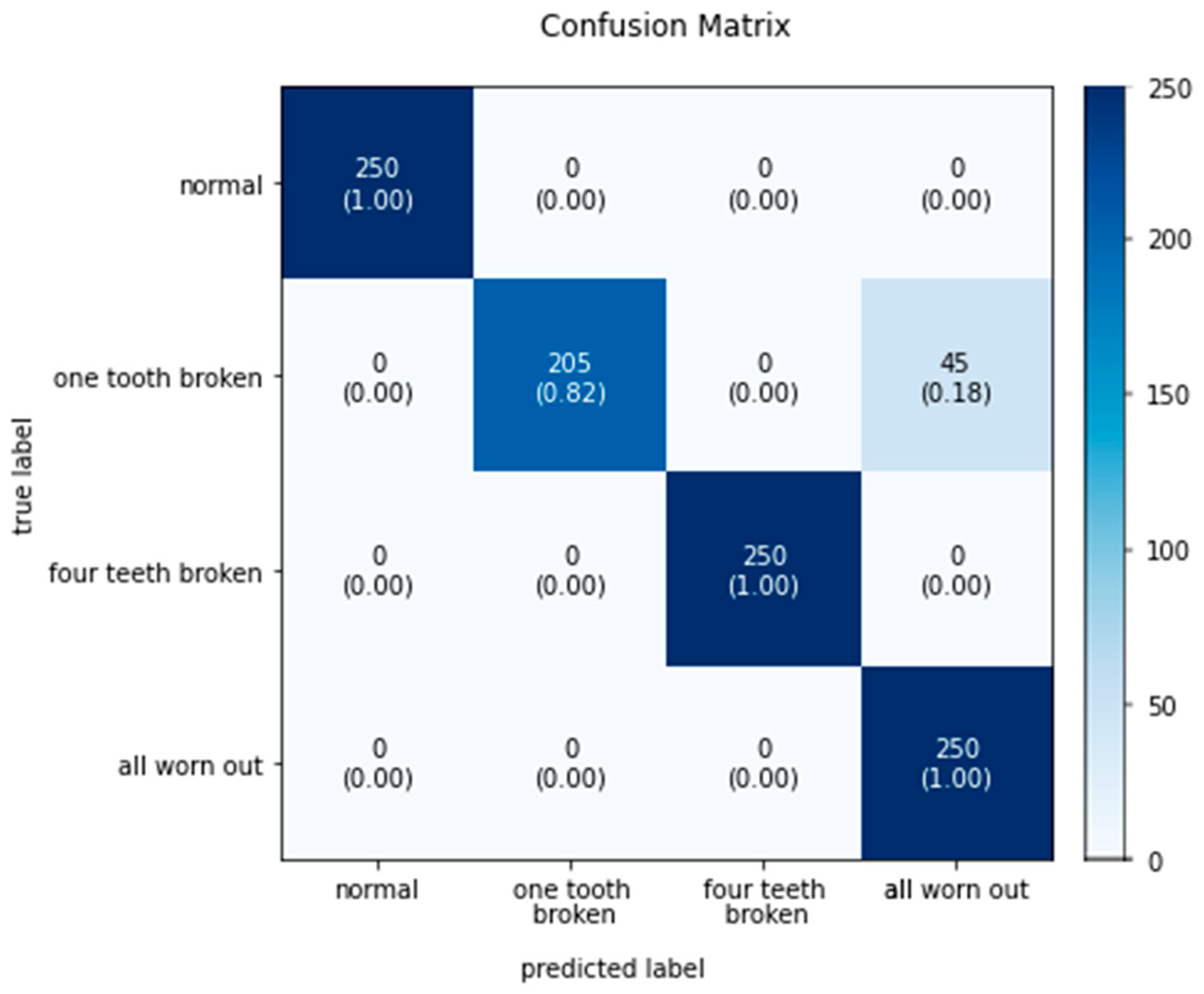
Figure 9 shows the confusion matrix of the proposed method. The overall classification accuracy was 95.5%. Note that normal gear and defective gears could be perfectly classified. However, ‘one tooth broken’ and ‘all worn out’ could not be exactly classified. Among the 250 samples of ‘one tooth broken’, 45 samples were predicted as an ‘all worn out’ gear, which seems to have been misclassified due to the similarity between the spectrum of the two cases. From Figure 1, it is shown that the ‘one tooth broken’ case and ‘all worn out’ case show similar results; therefore, the model misclassified 45 samples. However, we note that the model still shows 100% accuracy of comparison between normal gear and broken gear.

3.3. Comparison between CNN Classifiers

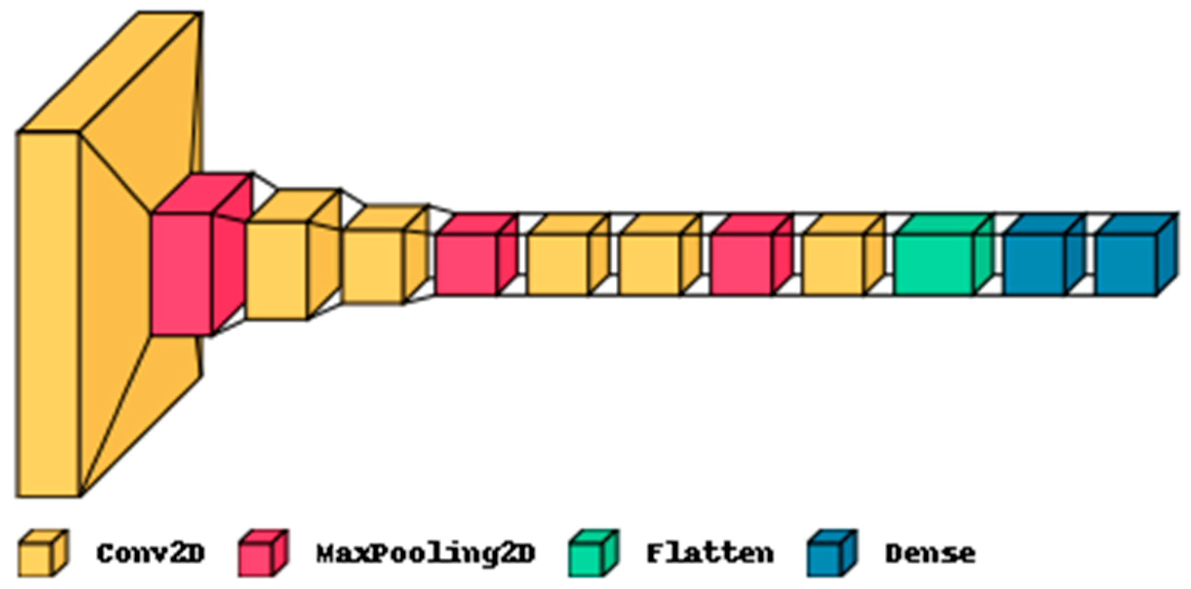
We compare the proposed method with the existing CNN classifier regarding the gear defect classification accuracy and computation time. Figure 10 shows the process of the comparison. The same data augmentation method was used for the sound data in Section 2.1, and the corresponding data are converted into a spectrogram image. The architecture of the CNN classifier used for comparison is shown in Table 4 and Figure 11 [43].
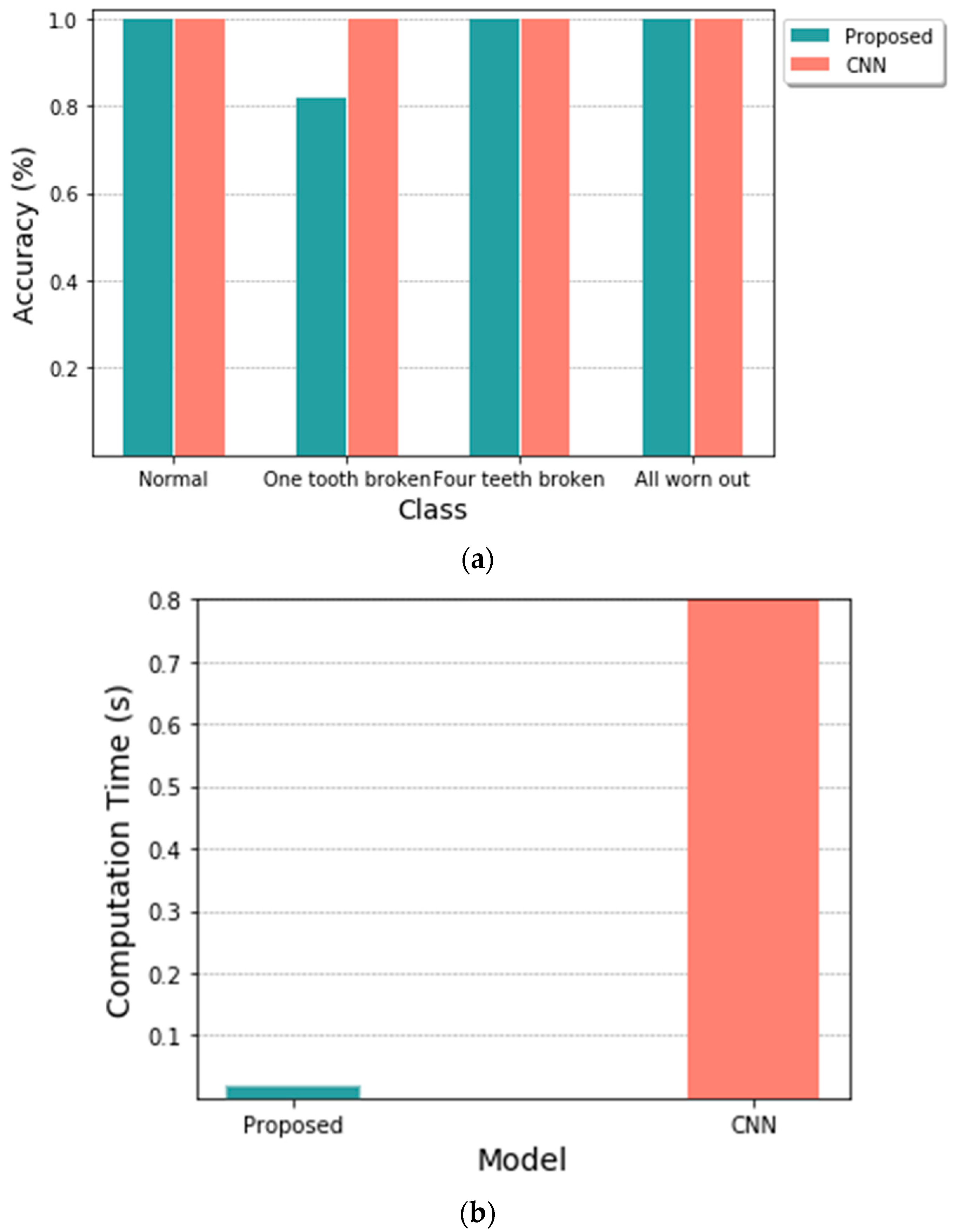
Figure 12a shows the classification accuracy by class for the test dataset. The ‘one tooth broken’ accuracy was 82%, which was lower in the proposed method than in CNN. However, both methods could classify normal gear and defective gears.
The calculation time from the moment the sound data are converted to the output of the diagnostic result was calculated, and shown in Table 5. One thousand data were diagnosed, and the computation time required per datum was calculated. We note that the computation time includes the data processing time, such as Fourier transform. In the case of CNN, the 2D image is input, so the acoustic data must be converted into a spectrogram image. The STFT used at this time has a difference in computational time during the conversion process because it performs FFT in short units several times. In addition, compared to DNN whose input size was 5 with 1D, CNN has a much larger size of 30 × 30 with a 2D image, as well as a convolution layer, which increases computational time.
Generally, CNN uses 2D input; therefore, the complexity of the model, the number of parameters, and the calculation process are much higher than the DNN model. As expected, the results showed that the proposed method using DNN took an average of 18.48 ms computation time per datum, and 0.80 s when spectrogram images were used as input to the CNN model. All data recorded the gear sound for 1 s, and in the case of CNN models, real-time diagnosis was difficult, and it was verified that the proposed method was sufficiently capable of real-time diagnosis.

4. Conclusions

In this paper, we propose a system for diagnosing gear defects through frequency analysis based on DNN. In the acoustic data, only the sums of frequency bands of interest are used as a feature that distinguishes the type of defect, and these features are used as inputs to a simple DNN model to reduce computation. Compared to CNN-based model methods, unnecessary data are not used for defect diagnosis, so computation can be reduced to diagnose defects in the gear in real-time. Although the existing defect diagnosis method using the CNN model was difficult to diagnose in real time in the computational environment without GPU due to a high computational volume, the proposed system can diagnose defects in real time without difficulty even with only a low-performance CPU.
The performance of the proposed system was evaluated using the sound of gears operating in real time as the test data. In addition, we verified classification accuracy and real-time defect diagnosis-capable processing speed by comparing the conventional sound-based defect diagnosis method, spectrogram images, as inputs to CNN models. It showed 95.5% accuracy for 1000 test data, and it took 18.48 ms—which is 40 times higher in speed compared to CNN model—to diagnose one gear sound data per second, enabling real-time diagnosis in a low-spec environment.
The proposed system has a limitation in that it cannot be classified in the case of new defect types by conducting learning and experiments only on limited defect types. However, it has been shown to have sufficient performance to classify normal and defective gears. In addition, the model successfully classified normal gears of different RPMs with minimum computational resources.
The system proposed in this paper is expected to be able to diagnose defects in real time at a relatively low cost, so it can be effectively used to diagnose various sound-based facilities in real time. As a future research plan, we plan to study a defect diagnosis system that is resistant to noise by considering the noise of the surrounding equipment.

Author Contributions

Conceptualization, J.K. (Jeonghyeon Kim), J.K. (Jonghoek Kim) and H.K.; methodology, J.K. (Jeonghyeon Kim) and H.K.; software, J.K. (Jeonghyeon Kim); validation, H.K.; formal analysis, J.K. (Jeonghyeon Kim) and H.K.; investigation, H.K.; resources, J.K. (Jeonghyeon Kim); data curation, J.K. (Jeonghyeon Kim); writing—original draft preparation, J.K. (Jeonghyeon Kim) and H.K.; writing—review and editing, J.K. (Jeonghyeon Kim) and H.K.; visualization, J.K. (Jeonghyeon Kim) and H.K.; supervision, J.K. (Jonghoek Kim) and H.K.; project administration, J.K. (Jonghoek Kim) and H.K. All authors have read and agreed to the published version of the manuscript.

Funding

This research was supported by the National Research Foundation of Korea (NRF) grant funded by the Korea Government (MSIT) under Grant 2021R1F1A1052193, and in part by the 2022 Hongik University Research Fund.

Institutional Review Board Statement

Not applicable.

Informed Consent Statement

Not applicable.

Data Availability Statement

Data are available within the article.

Conflicts of Interest

The funders had no role in the design of the study; in the collection, analyses, or interpretation of data; in the writing of the manuscript; or in the decision to publish the results.

References

  1. Cooper, C.; Kaplinsky, R. Technology and Development in the Third Industrial Revolution; Routledge: London, UK, 2005. [Google Scholar]
  2. Mowery, D.C. Plus ca change: Industrial R&D in the “third industrial revolution”. Ind. Corp. Change 2009, 18, 1–50. [Google Scholar]
  3. Greenwood, J. The Third Industrial Revolution: Technology, Productivity, and Income Inequality; Number 435; American Enterprise Institute: Washington, DC, USA, 1997. [Google Scholar]
  4. Carlsson, B. Technological Systems and Economic Performance: The Case of Factory Automation; Springer Science & Business Media: Berlin/Heidelberg, Germany, 2012; Volume 5. [Google Scholar]
  5. Wang, B.; Tao, F.; Fang, X.; Liu, C.; Liu, Y.; Freiheit, T. Smart manufacturing and intelligent manufacturing: A comparative review. Engineering 2021, 7, 738–757. [Google Scholar] [CrossRef]
  6. Dotoli, M.; Fay, A.; Mi’skowicz, M.; Seatzu, C. An overview of current technologies and emerging trends in factory automation. Int. J. Prod. Res. 2019, 57, 5047–5067. [Google Scholar] [CrossRef]
  7. Majchrzak, A. The Human Side of Factory Automation: Managerial and Human Resource Strategies for Making Automation Succeed; Jossey-Bass: Hoboken, NJ, USA, 1988. [Google Scholar]
  8. Jäntti, M.; Toroi, T.; Eerola, A. Difficulties in establishing a defect management process: A case study. In Proceedings of the International Conference on Product Focused Software Process Improvement, Amsterdam, The Netherlands, 12–14 June 2006; Springer: Berlin/Heidelberg, Germany, 2006; pp. 142–150. [Google Scholar]
  9. Adams, R.; Cawley, P.; Pye, C.; Stone, B. A vibration technique for non-destructively assessing the integrity of structures. J. Mech. Eng. Sci. 1978, 20, 93–100. [Google Scholar] [CrossRef]
  10. Maraaba, L.S.; Twaha, S.; Memon, A.; Al-Hamouz, Z. Recognition of stator winding inter-turn fault in interior-mount LSPMSM using acoustic signals. Symmetry 2020, 12, 1370. [Google Scholar] [CrossRef]
  11. Zaki, A.; Chai, H.K.; Aggelis, D.G.; Alver, N. Non-destructive evaluation for corrosion monitoring in concrete: A review and capability of acoustic emission technique. Sensors 2015, 15, 19069–19101. [Google Scholar] [CrossRef]
  12. Qian, S.; Chen, D. Joint time-frequency analysis. IEEE Signal Process. Mag. 1999, 16, 52–67. [Google Scholar] [CrossRef]
  13. Wyse, L. Audio spectrogram representations for processing with convolutional neural networks. arXiv 2017, arXiv:1706.09559. [Google Scholar]
  14. Hess-Nielsen, N.; Wickerhauser, M.V. Wavelets and time-frequency analysis. Proc. IEEE 1996, 84, 523–540. [Google Scholar] [CrossRef] [Green Version]
  15. Muda, L.; Begam, M.; Elamvazuthi, I. Voice recognition algorithms using mel frequency cepstral coefficient (MFCC) and dynamic time warping (DTW) techniques. arXiv 2010, arXiv:1003.4083. [Google Scholar]
  16. Kang, M.; Kim, J.; Wills, L.M.; Kim, J.M. Time-Varying and Multiresolution Envelope Analysis and Discriminative Feature Analysis for Bearing Fault Diagnosis. IEEE Trans. Ind. Electron. 2015, 62, 7749–7761. [Google Scholar] [CrossRef]
  17. Feng, Z.; Chen, X.; Wang, T. Time-varying demodulation analysis for rolling bearing fault diagnosis under variable speed conditions. J. Sound Vib. 2017, 400, 71–85. [Google Scholar] [CrossRef]
  18. Stefani, A.; Bellini, A.; Filippetti, F. Diagnosis of Induction Machines’ Rotor Faults in Time-Varying Conditions. IEEE Trans. Ind. Electron. 2009, 56, 4548–4556. [Google Scholar] [CrossRef]
  19. Zhou, K.; Tang, J. Harnessing fuzzy neural network for gear fault diagnosis with limited data labels. Int. J. Adv. Manuf. Technol. 2021, 115, 1005–1019. [Google Scholar] [CrossRef]
  20. Zhang, W.; Peng, G.; Li, C.; Chen, Y.; Zhang, Z. A new deep learning model for fault diagnosis with good anti-noise and domain adaptation ability on raw vibration signals. Sensors 2017, 17, 425. [Google Scholar] [CrossRef]
  21. Zhang, W.; Li, C.; Peng, G.; Chen, Y.; Zhang, Z. A deep convolutional neural network with new training methods for bearing fault diagnosis under noisy environment and different working load. Mech. Syst. Signal Process. 2018, 100, 439–453. [Google Scholar] [CrossRef]
  22. Allam, A.; Moussa, M.; Tarry, C.; Veres, M. Detecting Teeth Defects on Automotive Gears Using Deep Learning. Sensors 2021, 21, 8480. [Google Scholar] [CrossRef]
  23. Li, X.; Li, J.; Qu, Y.; He, D. Gear Pitting Fault Diagnosis Using Integrated CNN and GRU Network with Both Vibration and Acoustic Emission Signals. Appl. Sci. 2019, 9, 768. [Google Scholar] [CrossRef] [Green Version]
  24. Liu, H.; Li, L.; Ma, J. Rolling bearing fault diagnosis based on STFT-deep learning and sound signals. Shock. Vib. 2016, 2016, 6127479. [Google Scholar] [CrossRef] [Green Version]
  25. Verstraete, D.; Ferrada, A.; Droguett, E.L.; Meruane, V.; Modarres, M. Deep learning enabled fault diagnosis using time-frequency image analysis of rolling element bearings. Shock. Vib. 2017, 2017, 5067651. [Google Scholar] [CrossRef]
  26. Kang, K.W.; Lee, K.M. CNN-based Automatic Machine Fault Diagnosis Method Using Spectrogram Images. J. Inst. Converg. Signal Process. 2020, 21, 121–126. [Google Scholar]
  27. Kim, M.S.; Yun, J.P.; Park, P.G. Supervised and Unsupervised Learning Based Fault Detection Using Spectrogram. 2019. Available online: https://www.dbpia.co.kr/journal/articleDetail?nodeId=NODE09306024 (accessed on 2 August 2022).
  28. Nam, J.; Park, H.J. A Neural Network based Fault Detection and Classification System Using Acoustic Measurement. J. Korean Soc. Manuf. Technol. Eng. 2020, 29, 210–215. [Google Scholar]
  29. Yun, J.P.; Kim, M.S.; Koo, G.; Shin, W. Fault Diagnosis and Analysis Based on Transfer Learning and Vibration Signals. IEMEK J. Embed. Syst. Appl. 2019, 14, 287–294. [Google Scholar]
  30. Shen, S.; Lu, H.; Sadoughi, M.; Hu, C.; Nemani, V.; Thelen, A.; Webster, K.; Darr, M.; Sidon, J.; Kenny, S. A physics-informed deep learning approach for bearing fault detection. Eng. Appl. Artif. Intell. 2021, 103, 104295. [Google Scholar] [CrossRef]
  31. Shrestha, A.; Mahmood, A. Review of deep learning algorithms and architectures. IEEE Access 2019, 7, 53040–53065. [Google Scholar] [CrossRef]
  32. Titze, I.R.; Winholtz, W.S. Effect of microphone type and placement on voice perturbation measurements. J. Speech Lang. Hear Res. 1993, 36, 1177–1190. [Google Scholar] [CrossRef]
  33. Pham, H. Pyaudio: Portaudio v19 Python Bindings. 2006. Available online: https://people.csail.mit.edu/hubert/pyaudio (accessed on 2 August 2022).
  34. Landau, H. Sampling, data transmission, and the Nyquist rate. Proc. IEEE 1967, 55, 1701–1706. [Google Scholar] [CrossRef]
  35. Rebuffi, S.A.; Gowal, S.; Calian, D.A.; Stimberg, F.; Wiles, O.; Mann, T.A. Data augmentation can improve robustness. Adv. Neural Inf. Process. Syst. 2021, 34, 29935–29948. [Google Scholar]
  36. Psobot, Pedalboard, GitHub Repository. 2021. Available online: https://github.com/spotify/pedalboard (accessed on 27 July 2022).
  37. Eklund, V.V. Data Augmentation Techniques for Robust Audio Analysis. Master’s Thesis, Tampere University, Tampere, Finland, 2019. [Google Scholar]
  38. István, L.; Vér, L.L.B. Noise and Vibration Control Engineering: Principles and Applications; John Wiley Sons: Hoboken, NJ, USA, 2005. [Google Scholar]
  39. Van Der Walt, S.; Colbert, S.C.; Varoquaux, G. The NumPy array: A structure for efficient numerical computation. Comput. Sci. Eng. 2011, 13, 22–30. [Google Scholar] [CrossRef] [Green Version]
  40. Khor, J.Z.S.; Gopalai, A.A.; Lan, B.L.; Gouwanda, D.; Ahmad, S.A. The effects of mechanical noise bandwidth on balance across flat and compliant surfaces. Sci. Rep. 2021, 11, 12276. [Google Scholar] [CrossRef]
  41. Sola, J.; Sevilla, J. Importance of input data normalization for the application of neural networks to complex industrial problems. IEEE Trans. Nucl. Sci. 1997, 44, 1464–1468. [Google Scholar] [CrossRef]
  42. Komer, B.; Bergstra, J.; Eliasmith, C. Hyperopt-sklearn: Automatic hyperparameter configuration for scikit-learn. In Proceedings of the ICML Workshop on AutoML, Austin, TX, USA, 6–13 July 2006; Citeseer: Austin, TX, USA, 2014; Volume 9, p. 50. [Google Scholar]
  43. Solanki, A.; Pandey, S. Music instrument recognition using deep convolutional neural networks. Int. J. Inf. Technol. 2019, 14, 1659–1668. [Google Scholar] [CrossRef]
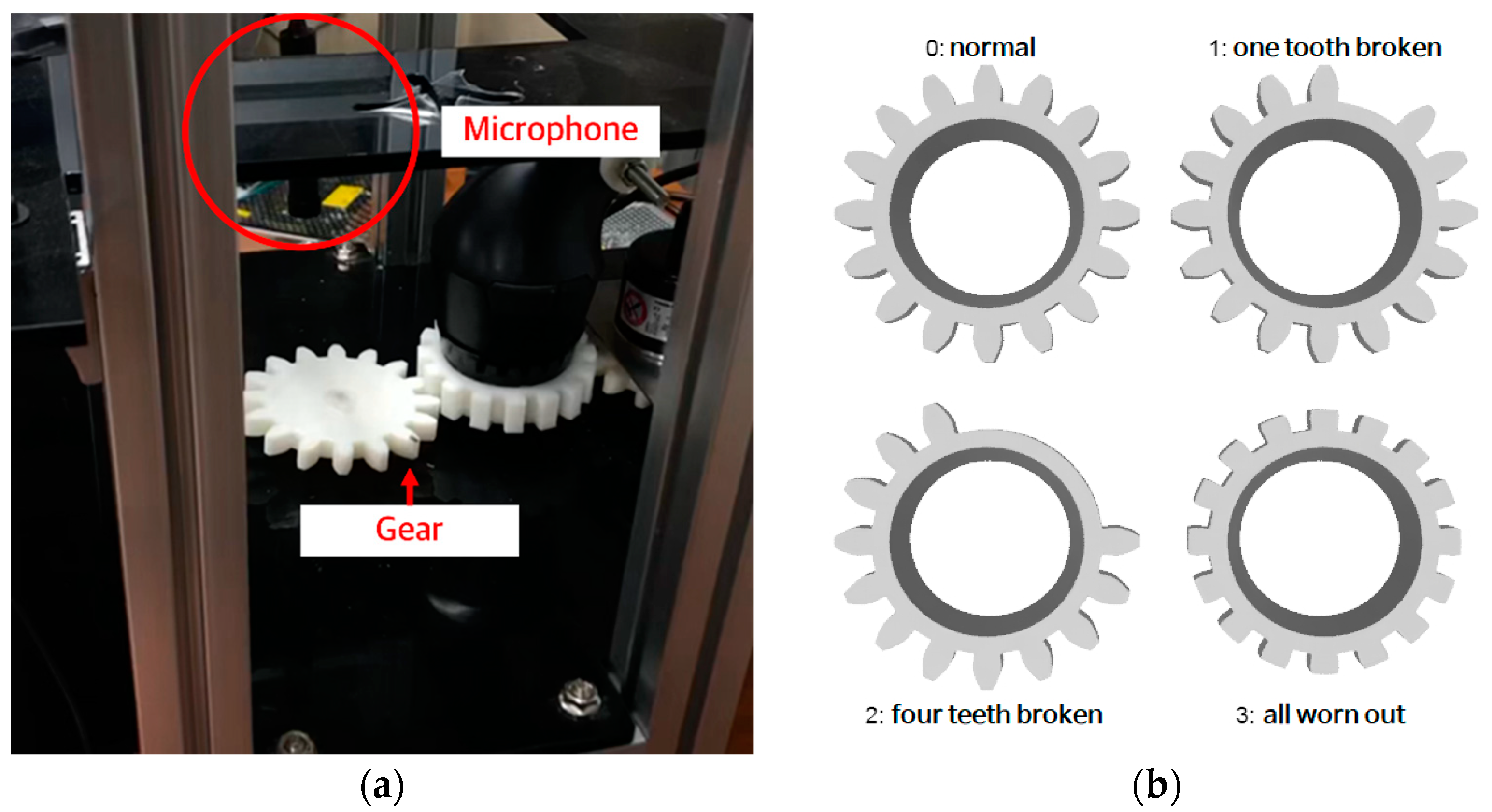
Figure 1. Setting for a gear’s defect diagnosis: (a) hardware for defect diagnosis; (b) type of normal gear and defect gears.
Machines 10 00659 g001
Figure 2. The overall flow of the gear’s defect diagnosis system.
Machines 10 00659 g002
Figure 3. Flow chart of sound spectrum analysis for classifier model training.
Machines 10 00659 g003
Figure 4. (a) Total of 150 samples of acoustic data in terms of frequency for each case. (b) Averaged frequency data for each gear case and frequency band selection example.
Machines 10 00659 g004aMachines 10 00659 g004b
Figure 5. The accuracy of training and validation sets for different selections of frequency bands: (a) case 1; (b) case 2; and (c) case 3.
Machines 10 00659 g005
Figure 6. DNN architecture for defect diagnosis.
Machines 10 00659 g006
Figure 7. The accuracy of training and validation sets without dropout layer.
Machines 10 00659 g007
Figure 8. Accuracy and loss function within 1000 training steps: (a) the train accuracy and the validation accuracy; (b) the train loss function and the validation loss function.
Machines 10 00659 g008aMachines 10 00659 g008b
Figure 9. Confusion matrix of the test set calculated by the trained model.
Machines 10 00659 g009
Figure 10. Comparison flow chart with the existing classifier.
Machines 10 00659 g010
Figure 11. The visualized architecture of CNN model.
Machines 10 00659 g011
Figure 12. Comparison of proposed DNN model and CNN model: (a) accuracy in test dataset; (b) computation time per data.
Machines 10 00659 g012
Table 1. Frequency band of interest in each case (Hz).
Frequency Selection Case 1Frequency Selection Case 2Frequency Selection Case 3
200~700200~7001900~2400
1000~15001000~15002400~2900
1700~22001700~22003000~3500
2200~27002200~27003800~4300
3500~45003000~35005500~6500
N/A3500~45007000~8000
Table 2. Model architecture summary.
LayerOutput ShapeParameter
Dense(None, 64)384
Dropout(None, 64)0
Dense(None, 64)4160
Dropout(None, 64)0
Dense(None, 4)260
Table 3. Hardware specifications.
OSCPURAM
Windows 10 Edu 64 bitIntel i3-7100U 2.4 GHz8 GB
Table 4. The details of the CNN model.
Layer (Type)Output ShapeParameter
conv2d (Conv2D)(None, 150, 150, 32)896
max_pooling2d(None, 50, 50, 32)0
conv2d (Conv2D)(None, 48, 48, 32)9248
max_pooling2d(None, 15, 15, 32)0
conv2d (Conv2D)(None, 13, 13, 32)9248
conv2d (Conv2D)(None, 11, 11, 64)18,496
max_pooling2d(None, 3, 3, 64)0
conv2d (Conv2D)(None, 1, 1, 64)36,928
flatten (Flatten)(None, 64)0
dense (Dense)(None, 64)4160
dense (Dense)(None, 4)260
Table 5. Comparison of computation time per data.
Proposed (DNN)CNN
18.48 ms0.80 s
Publisher’s Note: MDPI stays neutral with regard to jurisdictional claims in published maps and institutional affiliations.