Dynamic Simulation and Experimental Study of Electric Vehicle Motor-Gear System Based on State Space Method

Abstract

In the research on electric vehicle transmission vibration characteristics, the dynamic model involving a multistage gear system is still rare, especially the influences of driving motor excitation and load excitation which are not considered, and which makes the gear system research deviate from the actual situation. In addition, the changing processes of variables are usually simplified or neglected in the study of gear systems, which is not conducive in revealing the mechanism of gear dynamic behavior. In this paper, an improved dynamic model of a motor-gear system is established. The influences of driving motor excitation and load excitation are included, and the changing processes of tangential, axial, and torsional vibration variables of driving gear and driven gear are obtained using the state space method. Furthermore, the transmission housing vibration responses are investigated. By comparing the simulation results with the measurement data, the improved dynamic model, as well as the state space solution method, are verified as reliable and universal. On this basis, the influence of motor excitation on the state change of the gear system is discussed, which provides a theoretical approach for further study of motor drive gear systems.

1. Introduction

With the development of electric vehicles, the vibration characteristics of gear systems under electric motor driving conditions have become a research hotspot. The research on gear system dynamic characteristics is mainly from three aspects: inherent characteristics, dynamic response, and dynamic stability. Chen et al. [1] analyzed the relationship between the inherent characteristics of planetary gear transmissions and the meshing stiffness. The meshing stiffness has little effect on the low natural frequency less than 4000 Hz and has a relatively large effect on the high order natural frequency. Luo [2] studied the heat effect on the dynamic characteristics of gear transmission systems. The gear involute profile and the gear meshing stiffness were changed under different heat conditions. Zhu [3] investigated dynamical characteristics of wind turbine gearboxes with flexible pins. Decreasing the stiffness of flexible pins can reduce the amount of low frequency components and decrease the amplitude of vibrations.

Dynamic response mainly studies the dynamic excitation transfer process in the system and the state change of each component in the transmission system. Guo [4] established a refined single pair gear dynamic model considering time-varying mesh stiffness, backlash, and oil film force. The potential energy method was used to calculate time-varying mesh stiffness. The results show that backlash and torque fluctuation had significant impact on the gear pair. Cao [5] studied transmission acoustic performance in two aspects, excitation inhibition and noise transfer control. Through gear micro-geometry modification and transmission housing topological optimization, the transmission noise and vibration were both improved. Wei [6] took the influence of the uncertain parameters of gear transmission systems into consideration. The uncertain parameters included the moment of inertia of each component, the mesh stiffness, the mesh damping, and the transmission error, etc. Inalpolat [7] investigated the effect of gear tooth indexing errors on the dynamic response. The unfiltered raw transmission error and the high-pass filtered transmission error were obtained. Duan [8] proposed a rigid-flexible coupling dynamic model and calculated the transmission error. The root mean square amplitudes of the experimental transmission error was slightly larger than the theoretical transmission error.

When the gear system is in a state of instability, it will have a serious impact on the noise, stability, and reliability of the system. The stability of gear system parameters mainly includes the stability of the motion state and the stability of the vibration intensity. Garambois [9] investigated the NVH (noise, vibration, and harshness) robustness of gear optimization. The optimization was performed using a genetic algorithm, and the global design space was explored. Wang [10] established an analysis model including gear backlash, static transmission error, time-varying meshing stiffness, and stick-slip oscillation. The conclusion pointed out the boundaries that separate stable and unstable regions. Wang [11] established a dynamic model which contains a multistage gear transmission system. By analyzing the change of the Poincaré section, the sub-harmonic resonance and instability conditions were investigated. Abboudi [12] investigated a two-stage spur gear system by developing a lamped mass dynamic model with 12 DOFs (degrees of freedom). The differential equations were solved by an implicit Newmark algorithm. Walha [13] established a nonlinear dynamic model containing a two-stage helical gear system coupled with a clutch. This model possesses twenty-seven DOFs and includes three types of nonlinearity. The nonlinear equation was resolved by the analytic Runge–Kutta method. Cai [14,15] proposed gear mesh stiffness functions of both spur gears and helical gears. The helical gear mesh stiffness function was derived from the imitation of the ISO Standard 6336-1. Its change process presents a symmetrical exponential curve. Wei [16] calculated helical gear mesh stiffness by an improved analytical method. The results calculated by this method have little error with the results of the FEM method and ISO method.

Previous scholars have undertaken a lot of theoretical research on the dynamic modeling of cylindrical helical gears, but the dynamic research on the gear system of the pure electric vehicle multistage transmission is still rare, especially if the influence of drive motor excitation is not considered, which makes the simulation model deviate from the actual situation. Therefore, in this paper, an improved model is established considering the excitation of the driving motor, as well as two-stage meshing gear pairs.

However, the dynamic model of the multistage gear transmission is complex and difficult to solve, so the calculation and analysis of variables are usually simplified or neglected, which is not conducive to revealing the influence mechanism of gear dynamic behavior. In this paper, the state space method is introduced to solve the gear dynamics model of multistage transmission.

The state space describes the internal state of the system and the relationship between input and output. The state space method provides a convenient and simple solving method, which contains following advantages: (1) the state space method can not only reflect the changes of internal dynamic characteristics, but also reveal the relationship between the internal state and the external factors. (2) The state space method treats multiple variables as vectors, which is more suitable for solving the problem of multiple inputs and multiple output variables. Compared with other methods, the state space method covers a wide range for solving complex problems. As a result, the state space method is applicable to solve time-varying systems. Wu [17] presented a linear system with multiple exponential damping models. By using the extended state space formula, the dynamic responses were calculated. Lu [18] designed a proportional–integral–derivative controller based on a self-adaptive state space predictive functional control. The experimental results illustrated that the proposed method was better than other existing control methods. Demirhan [19] used the state space approach to investigate the bending and vibration characteristics of a porous plate. The effects of porosity parameter, the power-law index, and slenderness ratio on bending and vibration of the porous plate were calculated. Vaseghi [20] used the state space method to analyze electromagnetic scattering from anisotropic cylindrical structures. Scheel [21] used the polynomial nonlinear state space method to identify data-driven models.

Compared with the above research results, this paper contains the following creative works. First, a torsional vibration model of a motor-gear system is established, including motor, shafts, two-stage gear pairs, and load, which comprehensively considers the coupling effect of internal and external factors; secondly, the state space method of control theory is introduced to solve the torsional vibration model of the gear system, which improves the calculation efficiency; thirdly, the dynamic characteristics of the motor-gear system under different conditions are discussed, which provides a theoretical approach for further study of motor drive gear system.

2. Modeling Process

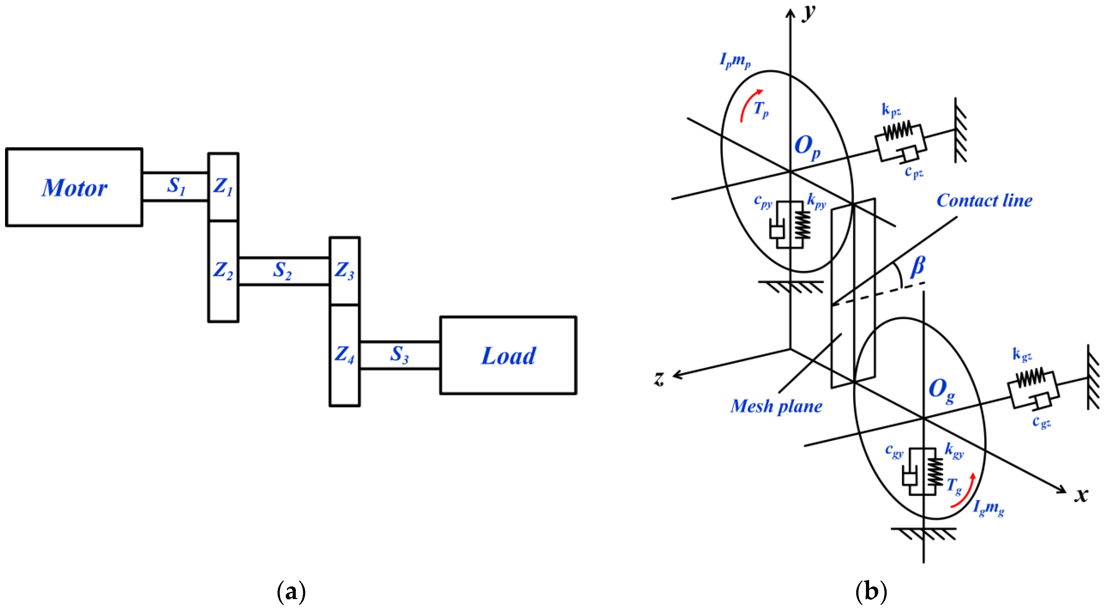
2.1. Improved Dynamic Model of Motor-Gear System

Dynamic excitation is the source of the gear system vibration, which can be divided into external and internal excitation. External excitation mainly refers to system input excitation, such as motor or engine torque fluctuation, and output excitation, such as load working condition. Internal excitation mainly contains time-varying mesh stiffness excitation and transmission error excitation. Time-varying mesh stiffness excitation is a kind of parametric excitation, which relates to gear design parameters such as tooth numbers, modules, helix angles, contact ratio, etc. Transmission error excitation is a kind of displacement excitation, which is caused by gear manufacture error and assembly error. By combining both external and internal excitation, the two-stage gear system dynamic model of electric vehicle transmission is shown in Figure 1.

Figure 1a displays the layout of the motor-gear system. For the helical gear system, since the meshing of gears produces an axial dynamic meshing force, the system will not only have torsional vibration and tangential vibration, but also cause axial vibration, resulting in bending-torsional-axial coupling vibration performance. As a result, the system is a three-dimensional vibration system.

Figure 1b displays the gear meshing dynamics without taking into account the frictional forces. For the motor-gear system dynamic model, we used the Lagrange equation to derive motion equations. The derivation of the dynamic equations can be found in Appendix A.

According to Figure 1b, assuming that the helix angle of the driving gear has a right rotation, and the helix angle is β, the relationship between the tangential vibration and axial vibration of the meshing point can be expressed as

$$z=y\tan \beta$$

(1)

Therefore, the generalized displacement array $\left\{\delta \right\}$ of the gear system can be expressed as

$$\left\{\delta \right\}={\left\{y_p{z}_p{\theta }_p{y}_g{z}_g{\theta }_g\right\}}^T$$

(2)

where y_p, z_p, θ_p, y_g, z_g, θ_g are the tangential vibration displacement, axial vibration displacement, and torsional vibration displacement of driving gear midpoint O_p and driven gear midpoint O_g in y direction and z direction, respectively. The relationship between the vibration displacement of meshing point P and the generalized displacement of the driving gear is

$${\overline{y}}_p=y_p+{\theta }_p{R}_p$$

(3)

$${\overline{z}}_p=z_p-{\overline{y}}_p\tan \beta =z_p-\left(y_p+{\theta }_p{R}_p\right)\tan \beta$$

(4)

The relationship between the vibration displacement of meshing point G and the generalized displacement of the driven gear is

$${\overline{y}}_g=y_g+{\theta }_g{R}_g$$

(5)

$${\overline{z}}_g=z_g-{\overline{y}}_g\tan \beta =z_g-\left(y_g+{\theta }_g{R}_g\right)\tan \beta$$

(6)

Therefore, the corresponding tangential dynamic meshing force F_y is

$$\begin{array}{ll}{F}_y& =k_{my}\left({\overline{y}}_p-{\overline{y}}_g-e_y\right)+c_{my}\left({\dot{\overline{y}}}_p-{\dot{\overline{y}}}_g-{\dot{\overline{e}}}_y\right)\\ & =\cos \beta [k_m\left(y_p+{\theta }_p{R}_p-y_g-{\theta }_g{R}_g-e_y\right)\\ & +c_m\left({\dot{y}}_p+R_p{\dot{\theta }}_p-{\dot{y}}_g-R_g{\dot{\theta }}_g-{\dot{e}}_y\right)]\end{array}$$

(7)

and the axial dynamic meshing force F_z is

$$\begin{array}{ll}{F}_z& =k_{mz}\left({\overline{z}}_p-{\overline{z}}_g-e_z\right)+c_{mz}\left({\dot{\overline{z}}}_p-{\dot{\overline{z}}}_g-{\dot{\overline{e}}}_z\right)\\ & =\sin \beta \{k_m\left[z_p-\tan \beta \left(y_p+{\theta }_p{R}_p\right)-z_g+\tan \beta \left(y_g+{\theta }_g{R}_g\right)-e_z\right]\\ & +c_m\left[{\dot{z}}_p-\tan \beta \left({\dot{y}}_p+R_p{\theta }_p\right)-{\dot{z}}_g+\tan \beta \left({\dot{y}}_g+R_g{\dot{\theta }}_g\right)-{\dot{e}}_z\right]\}\end{array}$$

(8)

where

$$\begin{array}{cc}{k}_{mz}=k_m\sin \beta & k_{my}=k_m\cos \beta \\ c_{mz}=c_m\sin \beta & c_{my}=c_m\cos \beta \\ e_z=e\sin \beta & e_y=e\cos \beta \end{array}\}$$

(9)

k_m is the normal meshing stiffness, c_m is the normal meshing damping, and e is the normal meshing error.

For motor tangential force F_My, it can be calculated according to following function [22]:

$$F_{My}=\frac{1}{2\mu }{B}_r{B}_{t}S$$

(10)

where μ is the air permeability, B_r is the radial air gap magnetic flux density, B_t is the tangential air gap magnetic flux density, and S is the inner effective surface area of stator core.

For motor axial force F_Mz, it consists of two items; one is caused by a skewed slot and the other is caused by the misalignment of stator and rotor [23]. The formula is listed below:

$$F_{Mz}=\frac{6P_{em}}{Nnl}\times {10}^4+\pi R\frac{\partial }{\partial h}\left[{\displaystyle \underset{l}{\int }{B}_{\delta }^2\left(h,l\right)dl}\right]$$

(11)

where P_em is the electromagnetic power, N is the number of slots, n is the motor speed, l is the effective length of stator core, R is the armature radius, $B_{\delta }^2\left(h,l\right)$ is the axial distribution function of air gap flux, and h is the stagger distance of stator and rotor.

During the bench test, the load of the transmission is also simulated by the motor. Therefore, the gear system is also affected by the tangential force and axial force of the load motor. The tangential force F_Ly and the axial force F_Lz can also be obtained by referring to Formulas (10) and (11).

For the first-stage gear pair Z₁ and Z₂, the dynamic functions are listed as follows:

$$m_{1Gp}{\ddot{y}}_{1Gp}+c_{1Gpy}{\dot{y}}_{1Gp}+k_{1Gpy}{y}_{1Gp}=-F_{1Gy}+F_{My}$$

(12)

$$m_{1Gp}{\ddot{z}}_{1Gp}+c_{1Gpz}{\dot{z}}_{1Gp}+k_{1Gpz}{z}_{1Gp}=F_{1Gz}-F_{Mz}$$

(13)

$$I_{1Gp}{\ddot{\theta }}_{1Gp}=\left(-F_{1Gy}+F_{My}\right)R_{1Gp}+T_M$$

(14)

$$m_{1Gg}{\ddot{y}}_{1Gg}+c_{1Ggy}{\dot{y}}_{1Gg}+k_{1Ggy}{y}_{1Gg}=F_{1Gy}-F_{My}$$

(15)

$$m_{1Gg}{\ddot{z}}_{1Gg}+c_{1Ggz}{\dot{z}}_{1Gg}+k_{1Ggz}{z}_{1Gg}=-F_{1Gz}+F_{Mz}$$

(16)

$$I_{1Gg}{\ddot{\theta }}_{1Gg}=\left(F_{1Gy}-F_{My}\right)R_{1Gg}-T_{1G}$$

(17)

For the second-stage gear pair Z₃ and Z₄, the dynamic functions are listed as follows:

$$m_{2Gp}{\ddot{y}}_{2Gp}+c_{2Gpy}{\dot{y}}_{2Gp}+k_{2Gpy}{y}_{2Gp}=-F_{2Gy}+F_{1Gy}-F_{Ly}$$

(18)

$$m_{2Gp}{\ddot{z}}_{2Gp}+c_{2Gpz}{\dot{z}}_{2Gp}+k_{2Gpz}{z}_{2Gp}=F_{2Gz}-F_{1Gz}+F_{Lz}$$

(19)

$$I_{2Gp}{\ddot{\theta }}_{2Gp}=\left(-F_{2Gy}+F_{1Gy}-F_{Ly}\right)R_{2Gp}+T_{1G}$$

(20)

$$m_{2Gg}{\ddot{y}}_{2Gg}+c_{2Ggy}{\dot{y}}_{2Gg}+k_{2Ggy}{y}_{2Gg}=F_{2Gy}-F_{1Gy}+F_{Ly}$$

(21)

$$m_{2Gg}{\ddot{z}}_{2Gg}+c_{2Ggz}{\dot{z}}_{2Gg}+k_{2Ggz}{z}_{2Gg}=-F_{2Gz}+F_{1Gz}-F_{Lz}$$

(22)

$$I_{2Gg}{\ddot{\theta }}_{2Gg}=\left(F_{2Gy}-F_{1Gy}+F_{Ly}\right)R_{2Gg}-T_{2G}$$

(23)

where the subscript 1G, 2G represent the meshing gear pair; p, g represent the driving gear and driven gear; y, z represent the tangential direction and axial direction; and M, L represent the motor and load.

By substituting Equations (7), (8), (10) and (11) into Equations (12)–(23), the dynamic functions of the first-stage gear pair and second-stage gear pair can be calculated. The detailed calculation process can be found in Appendix B.

The dynamic function can be expressed in the form of matrix:

$$\left[M_{iG}\right]\left\{{\ddot{\delta }}_{iG}\right\}+\left[C_{iG}\right]\left\{{\dot{\delta }}_{iG}\right\}+\left[K_{iG}\right]\left\{{\delta }_{iG}\right\}=\left\{P_{iG}\right\}$$

(24)

where M_iG, C_iG, K_iG, P_iG (i = 1, 2) are listed below:

$$\left[M_{iG}\right]=\left[\begin{array}{cccccc}{m}_{iGp}& & & & & \\ & m_{iGp}& & & 0& \\ & & I_{iGp}& & & \\ & & & m_{iGg}& & \\ & 0& & & m_{iGg}& \\ & & & & & I_{iGg}\end{array}\right]$$

(25)

$$\left[C_{iG}\right]=\left[\begin{array}{cccccc}{c}_{iGpy}+\cos {\beta }_{iG}{c}_{iGm}& 0& \cos {\beta }_{iG}{c}_{iGm}{R}_{iGp}& -\cos {\beta }_{iG}{c}_{iGm}& 0& -\cos {\beta }_{iG}{c}_{iGm}{R}_{iGg}\\ \sin {\beta }_{iG}\tan {\beta }_{iG}{c}_{iGm}& -\sin {\beta }_{iG}{c}_{iGm}+c_{iGpz}& -\sin {\beta }_{iG}\tan {\beta }_{iG}{c}_{iGm}{R}_{iGp}& -\sin {\beta }_{iG}\tan {\beta }_{iG}{c}_{iGm}& \sin {\beta }_{iG}{c}_{iGm}& -\sin {\beta }_{iG}\tan {\beta }_{iG}{c}_{iGm}{R}_{iGg}\\ \cos {\beta }_{iG}{c}_{iGm}{R}_{iGp}& 0& R_{iGp}^2\cos {\beta }_{iG}{c}_{iGm}& -\cos {\beta }_{iG}{c}_{iGm}{R}_{iGp}& 0& -R_{iGp}{R}_{iGg}\cos {\beta }_{iG}{c}_{iGm}\\ -\cos {\beta }_{iG}{c}_{iGm}& 0& -\cos {\beta }_{iG}{c}_{iGm}{R}_{iGp}& \cos \beta c_{iGm}+c_{iGgy}& 0& \cos {\beta }_{iG}{c}_{iGm}{R}_{iGg}\\ -\sin {\beta }_{iG}\tan {\beta }_{iG}{c}_{iGm}& \sin {\beta }_{iG}{c}_{iGm}& -\sin {\beta }_{iG}\tan {\beta }_{iG}{c}_{iGm}{R}_{iGp}& \sin {\beta }_{iG}\tan {\beta }_{iG}{c}_{iGm}& c_{iGgy}-\sin {\beta }_{iG}{c}_{iGm}& \sin {\beta }_{iG}\tan {\beta }_{iG}{c}_{iGm}{R}_{iGg}\\ -\cos {\beta }_{iG}{c}_{iGm}{R}_{iGg}& 0& -R_{iGp}{R}_{iGg}\cos {\beta }_{iG}{c}_{iGm}& \cos {\beta }_{iG}{c}_{iGm}{R}_{iGg}& 0& R_{iGg}^2\cos {\beta }_{iG}{c}_{iGm}\end{array}\right]$$

(26)

$$\left[K_{iG}\right]=\left[\begin{array}{cccccc}{k}_{iGpy}+\cos {\beta }_{iG}{k}_{iGm}& 0& \cos {\beta }_{iG}{k}_{iGm}{R}_{iGp}& -\cos {\beta }_{iG}{k}_{iGm}& 0& -\cos {\beta }_{iG}{k}_{iGm}{R}_{iGg}\\ \sin {\beta }_{iG}\tan {\beta }_{iG}{k}_{iGm}& -\sin {\beta }_{iG}{k}_{iGm}+k_{iGpz}& -\sin {\beta }_{iG}\tan {\beta }_{iG}{k}_{iGm}{R}_{iGp}& -\sin {\beta }_{iG}\tan {\beta }_{iG}{k}_{iGm}& \sin {\beta }_{iG}{k}_{iGm}& -\sin {\beta }_{iG}\tan {\beta }_{iG}{k}_{iGm}{R}_{iGg}\\ \cos {\beta }_{iG}{k}_{iGm}{R}_{iGp}& 0& R_{iGp}^2\cos {\beta }_{iG}{k}_{iGm}& -\cos {\beta }_{iG}{k}_{iGm}{R}_{iGp}& 0& -R_{iGp}{R}_{iGg}\cos {\beta }_{iG}{k}_{iGm}\\ -\cos {\beta }_{iG}{k}_{iGm}& 0& -\cos {\beta }_{iG}{k}_{iGm}{R}_{iGp}& \cos {\beta }_{iG}{k}_{iGm}+k_{iGgy}& 0& \cos {\beta }_{iG}{k}_{iGm}{R}_{iGg}\\ -\sin {\beta }_{iG}\tan {\beta }_{iG}{k}_{iGm}& \sin {\beta }_{iG}{k}_{iGm}& -\sin {\beta }_{iG}\tan {\beta }_{iG}{k}_{iGm}{R}_{iGp}& \sin {\beta }_{iG}\tan {\beta }_{iG}{k}_{iGm}& k_{iGgy}-\sin {\beta }_{iG}{k}_{iGm}& \sin {\beta }_{iG}\tan {\beta }_{iG}{k}_{iGm}{R}_{iGg}\\ -\cos {\beta }_{iG}{k}_{iGm}{R}_{iGg}& 0& -R_{iGp}{R}_{iGg}\cos {\beta }_{iG}{k}_{iGm}& \cos {\beta }_{iG}{k}_{iGm}{R}_{iGg}& 0& R_{iGg}^2\cos {\beta }_{iG}{k}_{iGm}\end{array}\right]$$

(27)

$$\left\{P_{1G}\right\}=\left\{\begin{array}{c}\cos {\beta }_{1G}\left(c_{1Gm}{\dot{e}}_{1Gy}+k_{1Gm}{e}_{1Gy}\right)+F_{My}\\ -\sin {\beta }_{1G}\left(c_{1Gm}{\dot{e}}_{1Gz}+k_{1Gm}{e}_{1Gz}\right)-F_{Mz}\\ R_{1Gp}\left[\cos {\beta }_{1G}\left(c_{1Gm}{\dot{e}}_{1Gy}+k_{1Gm}{e}_{1Gy}\right)+F_{My}\right]+T_M\\ -\cos {\beta }_{1G}\left(c_{1Gm}{\dot{e}}_{1Gy}+k_{1Gm}{e}_{1Gy}\right)-F_{My}\\ \sin {\beta }_{1G}\left(c_{1Gm}{\dot{e}}_{1Gz}+k_{1Gm}{e}_{1Gz}\right)+F_{Mz}\\ R_{1Gg}\left[-\cos {\beta }_{1G}\left(c_{1Gm}{\dot{e}}_{1Gy}+k_{1Gm}{e}_{1Gy}\right)-F_{My}\right]-T_{1G}\end{array}\right\}$$

(28)

$$\left\{P_{2G}\right\}=\left\{\begin{array}{c}\cos {\beta }_{2G}\left(c_{2Gm}{\dot{e}}_{2Gy}+k_{2Gm}{e}_{2Gy}\right)+F_{1Gy}-F_{Ly}\\ -\sin {\beta }_{2G}\left(c_{2Gm}{\dot{e}}_{2Gz}+k_{2Gm}{e}_{2Gz}\right)-F_{1Gz}+F_{Lz}\\ R_{2Gp}\left[\cos {\beta }_{2G}\left(c_{2Gm}{\dot{e}}_{2Gy}+k_{2Gm}{e}_{2Gy}\right)+F_1{}_{Gy}-F_{Ly}\right]+T_{1G}\\ -\cos {\beta }_{2G}\left(c_{2Gm}{\dot{e}}_{2Gy}+k_{2Gm}{e}_{2Gy}\right)-F_{1Gy}+F_{Ly}\\ \sin {\beta }_{2G}\left(c_{2Gm}{\dot{e}}_{2Gz}+k_{2Gm}{e}_{2Gz}\right)+F_{1Gz}-F_{Lz}\\ R_{2Gg}\left[-\cos {\beta }_{2G}\left(c_{2Gm}{\dot{e}}_{2Gy}+k_{2Gm}{e}_{2Gy}\right)-F_{1Gy}+F_{Ly}\right]-T_{2G}\end{array}\right\}$$

(29)

2.2. Model Parameters

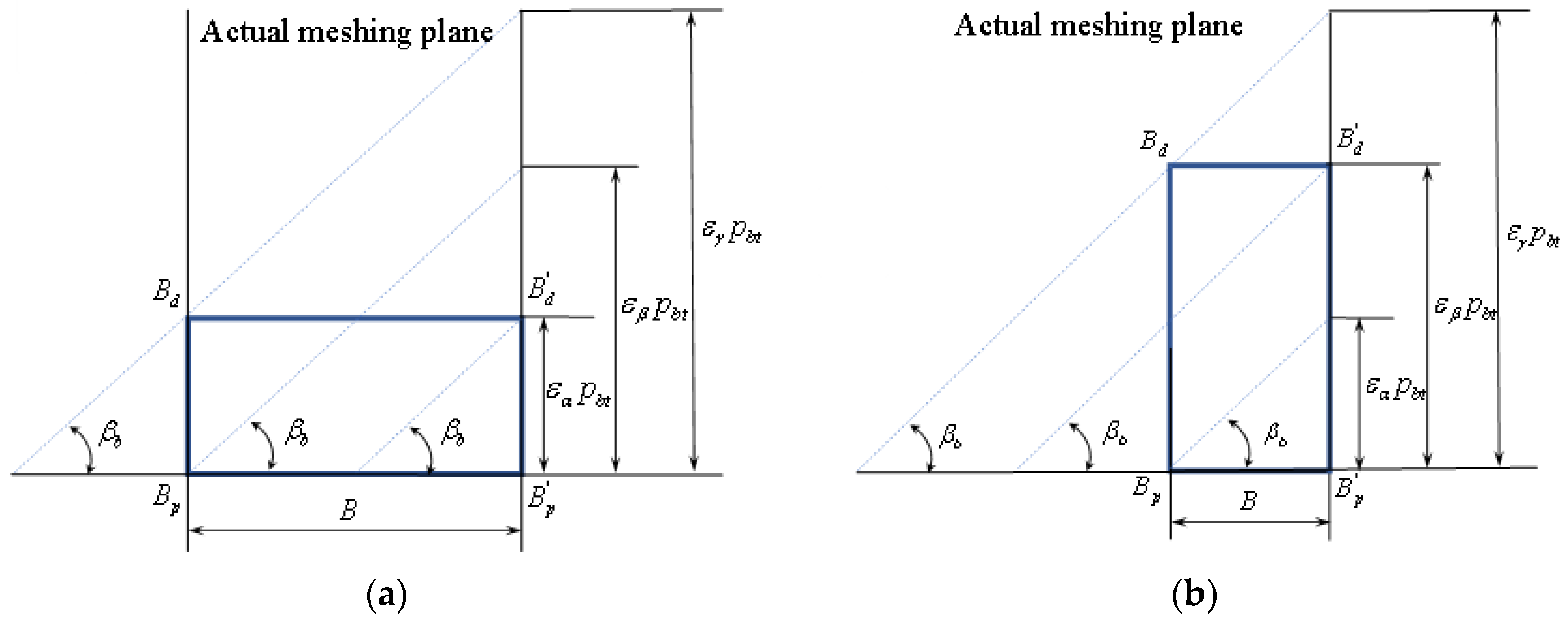
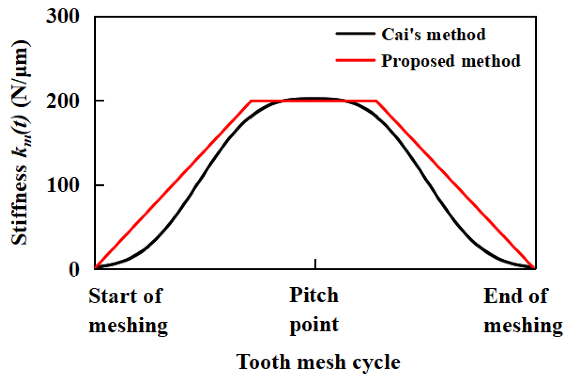
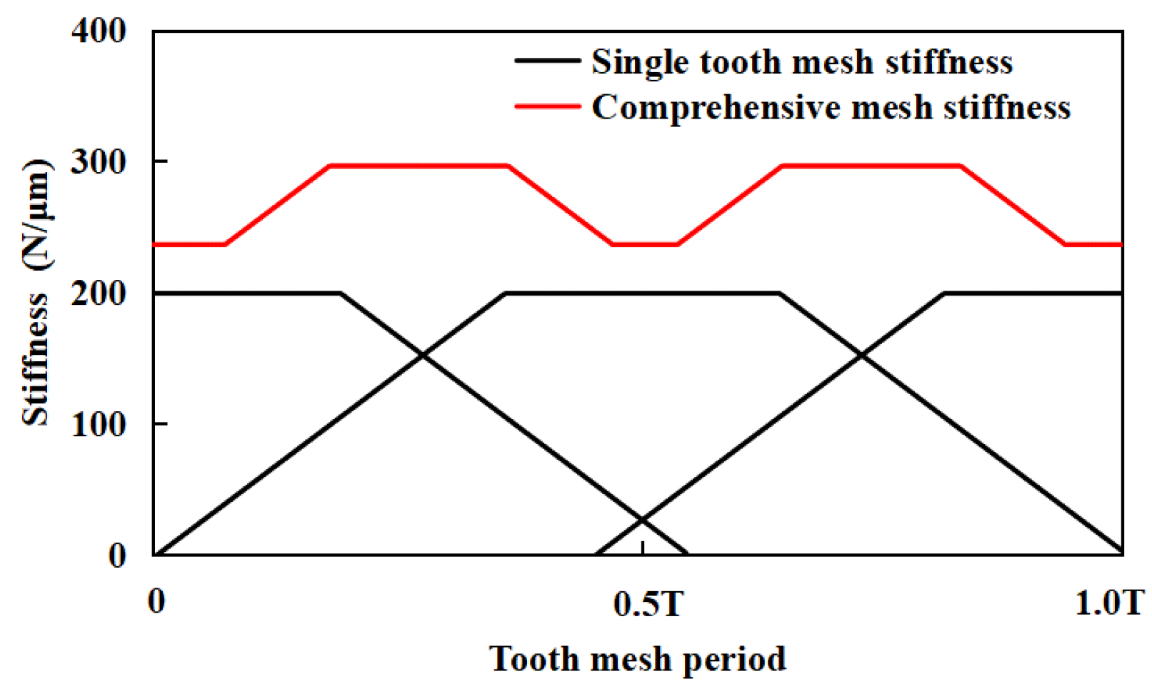
2.2.1. Stiffness

The meshing stiffness of the helical gear is related to the length of the contact line. According to the different relationships between tooth width and contact ratio, the length of the contact line can be concluded into following two types, as shown in Figure 2.

According to the geometric relationship of the meshing surface of the helical gear, the length of the contact line can be calculated by the following formula:

${\epsilon }_{\alpha }\le {\epsilon }_{\beta }$

$$l(i,t)=\{\begin{array}{c}\frac{p_{bt}}{\sin {\beta }_b}\cdot \frac{t}{T_M}\\ \frac{p_{bt}}{\sin {\beta }_b}\cdot {\epsilon }_{\alpha }\\ \frac{p_{bt}}{\sin {\beta }_b}({\epsilon }_{\gamma }-\frac{t}{T_M})\\ 0\end{array}\begin{array}{c}0\le \frac{t}{T_M}\le {\epsilon }_{\beta }\\ {\epsilon }_{\alpha }<\frac{t}{T_M}\le {\epsilon }_{\beta }\\ {\epsilon }_{\beta }<\frac{t}{T_M}\le {\epsilon }_{\gamma }\\ {\epsilon }_{\gamma }<\frac{t}{T_M}<ceil({\epsilon }_{\gamma })\end{array}$$

(30)

${\epsilon }_{\alpha }>{\epsilon }_{\beta }$

$$l(i,t)=\{\begin{array}{c}\frac{p_{bt}}{\sin {\beta }_b}\cdot \frac{t}{T_M}\\ \frac{p_{bt}}{\sin {\beta }_b}\cdot {\epsilon }_{\beta }\\ \frac{p_{bt}}{\sin {\beta }_b}({\epsilon }_{\gamma }-\frac{t}{T_M})\\ 0\end{array}\begin{array}{c}0\le \frac{t}{T_M}\le {\epsilon }_{\beta }\\ {\epsilon }_{\beta }<\frac{t}{T_M}\le {\epsilon }_{\alpha }\\ {\epsilon }_{\alpha }<\frac{t}{T_M}\le {\epsilon }_{\gamma }\\ {\epsilon }_{\gamma }<\frac{t}{T_M}<ceil({\epsilon }_{\gamma })\end{array}$$

(31)

where ε_α is the transverse contact ratio, ε_β is the axial contact ratio, ε_γ is the total contact ratio, p_bt is the base pitch, T_M is the meshing period, and ceil(ε_γ) is the minimum integer larger than ε_γ.

Therefore, the time-various length of contact line is expressed as

$$l(i,t)=l\left[1,t+(i-1)T_M\right]$$

(32)

Let M = ceil(ε_γ), the total time-various length of the contact line can be calculated by the following formula:

$$L(t)=l(1,t)+l(2,t)+\cdot \cdot \cdot +l(M,t)={\displaystyle \sum _{i=1}^{M}l(i,t)}$$

(33)

The unit meshing stiffness of the helical gear can be calculated.

For single stiffness c′,

$$c^{\prime }=0.8{c^{\prime }}_{th}{C}_R{C}_B\cos \beta$$

(34)

For mesh stiffness c_γ,

$$c_{\gamma }=c^{\prime }(0.75{\epsilon }_{\alpha }+0.25)$$

(35)

Therefore, the total time-varying meshing stiffness can be expressed as

$$k_m(t)=c_{\gamma }\cdot L(t)$$

(36)

The symbols in Equations (34)–(36) can be found in ISO 6336-1-2006.

According to the derivation of the above formula, the time-varying meshing stiffness function of the gear is a piecewise linear function, which is beneficial in solving the function by the state space method.

In order to verify the correctness of the time-varying meshing stiffness calculation method, the stiffness curve was compared with the Cai’s method in [15]. Take the first-stage gear pair Z₁ and Z₂ as an example; the two kinds of single tooth meshing stiffness curves are shown in Figure 3.

It can be seen from Figure 3 that the maximum values of the curve calculated by the two methods are very close, and the overall shapes of two curves are also similar. The main characteristics of meshing stiffness by the proposed method are proved consistent with meshing stiffness by Cai’s method. Therefore, the proposed mesh stiffness calculation method was verified a fairly correct method to solve helical gear mesh stiffness.

On this basis, the stiffness which contains multiple pairs of teeth meshing can be calculated. Figure 4 shows the curves of both single tooth mesh stiffness and multiple teeth comprehensive mesh stiffness. The time-varying stiffness curves illustrate the variable internal excitation, which is the most essential parameter excitation of the gear system.

2.2.2. Damping

The gear mesh damping can be calculated according to the following equation [24]:

$$c_m(t)=2{\xi }_g\sqrt{\frac{k_m(t)I_p{I}_g}{R_p^2{I}_p+R_g^2{I}_g}}$$

(37)

where ξ_g is the gear mesh damping ratio—the general value range is 0.03~0.17; R_p, R_g are the base radius of driving and driven gears; I_p, I_g are the moment of inertia of driving and driven gears.

2.2.3. Errors

It is inevitable to generate errors in the process of gear manufacturing. Gear errors mainly consist of three categories: pitch deviation, profile deviation, and helix deviation. Take a gear with a fifth level of accuracy as an example; its pitch deviation F_p, profile deviation F_α, and helix deviation F_β can be calculated according to the following equations [25].

$$F_p=0.3m+1.25\sqrt{d}+7$$

(38)

$$F_{\alpha }=3.2\sqrt{m}+0.22\sqrt{d}+0.7$$

(39)

$$F_{\beta }=0.1\sqrt{d}+0.63+\sqrt{b}+4.2$$

(40)

where m is normal modulus, d is reference diameter, and b is tooth width.

Converting the sum of the three errors into the normal meshing line can conclude the average error of the gear [26]. The comprehensive error can be expressed in the form of a sine function varying with time:

$$e(t)=e_0+e_a\sin ({\omega }_{h}t+\phi )$$

(41)

2.2.4. Elements

The element parameters of the gear system dynamic model, such as gears, shafts, and motor, are shown in

Table 1. Parameters of elements.

Elements	Parameters	Values
Gears	Gear No.	First-stage gear pair		Second-stage gear pair
		Gear Z1	Gear Z2	Gear Z3	Gear Z4
	Number of teeth	11	36	17	62
	Normal module (mm)	2.5		2.25
	Pressure angle (deg)	20		20
	Helix angle (deg)	25.5		30
	Face width (mm)	14.00	12.50	28.10	25.00
	Profile shift coefficient (mm)	0.35	−0.43	0.32	0.32
	Base diameter (mm)	28.26	92.48	40.72	148.50
	Reference diameter (mm)	30.47	99.71	44.17	161.08
	Tip diameter (mm)	38.25	102.00	51.30	167.41
	Root diameter (mm)	27.85	90.54	38.96	155.57
	Center distance (mm)	65		104
	Gear ratio	3.27		3.65
	Moment of inertia (kg·mm2)	13	865	89	6355
Shafts	Shaft No.	Shaft S1	Shaft S2		Shaft S3
	Diameter (mm)	23	30		40
	Length (mm)	82.5	61.1		82.9
Motor	Number of poles	10
	Number of slots	72
	Length of effective stator (mm)	240
	Armature radius (mm)	360
	Axial air gap flux (T)	0.84
	Air permeability (H/m)	4 × 10−7

.

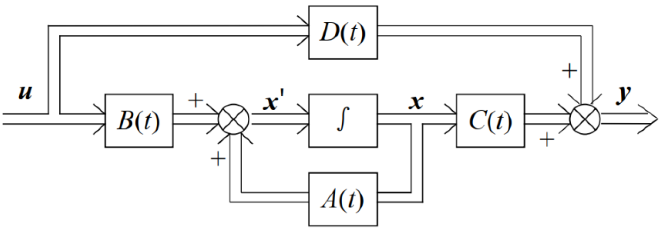
2.3. State Space Method

The state space method is a kind of control method that can reflect the changes of all independent variables of the system. All the internal motion states of the system can be obtained at the same time. In addition, the state space method has a wide range of applications. It is not only applicable to single input single output (SISO) linear constant systems, but also to multiple input multiple output (MIMO) systems, nonlinear systems, time-varying systems, and stochastic systems [27,28]. Furthermore, it can be easily solved in several seconds by using a digital computer and can even directly use the computer for real-time control, which shows its great advantages. Figure 5 shows the structure diagram of a MIMO linear time-varying system.

The dynamic characteristics of the system in Figure 5 can be described by the first-order differential equations composed of state variables. The mathematical expression is

$$\{\begin{array}{c}{x}^{\prime }=A(t)x+B(t)u\\ y=C(t)x+D(t)u\end{array}$$

(42)

where x is the state vector of n dimension, u is the input vector of r dimension, y is the output vector of m dimension, A is the system matrix of n × n dimension, B is the input matrix of n × r dimension, C is the output matrix of m × n dimension, and D is the direct matrix of m × r dimension.

Based on the expression of Formula (42), the gear system dynamic vibration Function (24) in Section 2.1 can be transformed accordingly.

Let $x=\left\{{\delta }_{iG}\right\}$, Function (24) can be expressed as:

$$\left[M_{iG}\right]\ddot{x}+\left[C_{iG}\right]\dot{x}+\left[K_{iG}\right]x=\left\{P_{iG}\right\}$$

(43)

Define

$$Y=\left[\begin{array}{c}x\\ \dot{x}\end{array}\right]$$

(44)

Thus, x and ẋ are composed of the state space, and Function (43) can be expressed as

$$\{\begin{array}{l}\dot{Y}=AY+B\left\{P_{iG}\right\}\\ Y=Y\end{array}$$

(45)

where $A=\left[\begin{array}{cc}{0}_{6\times 6}& I_{6\times 6}\\ -M_{iG}{}^{-1}{K}_{iG}& -M_{iG}{}^{-1}{C}_{iG}\end{array}\right]$, $B=\left[\begin{array}{c}{0}_{6\times 6}\\ M_{iG}{}^{-1}\end{array}\right]$.

By solving the above state space function with a computer program or mathematical tools, the process of variable changing with time can be obtained.

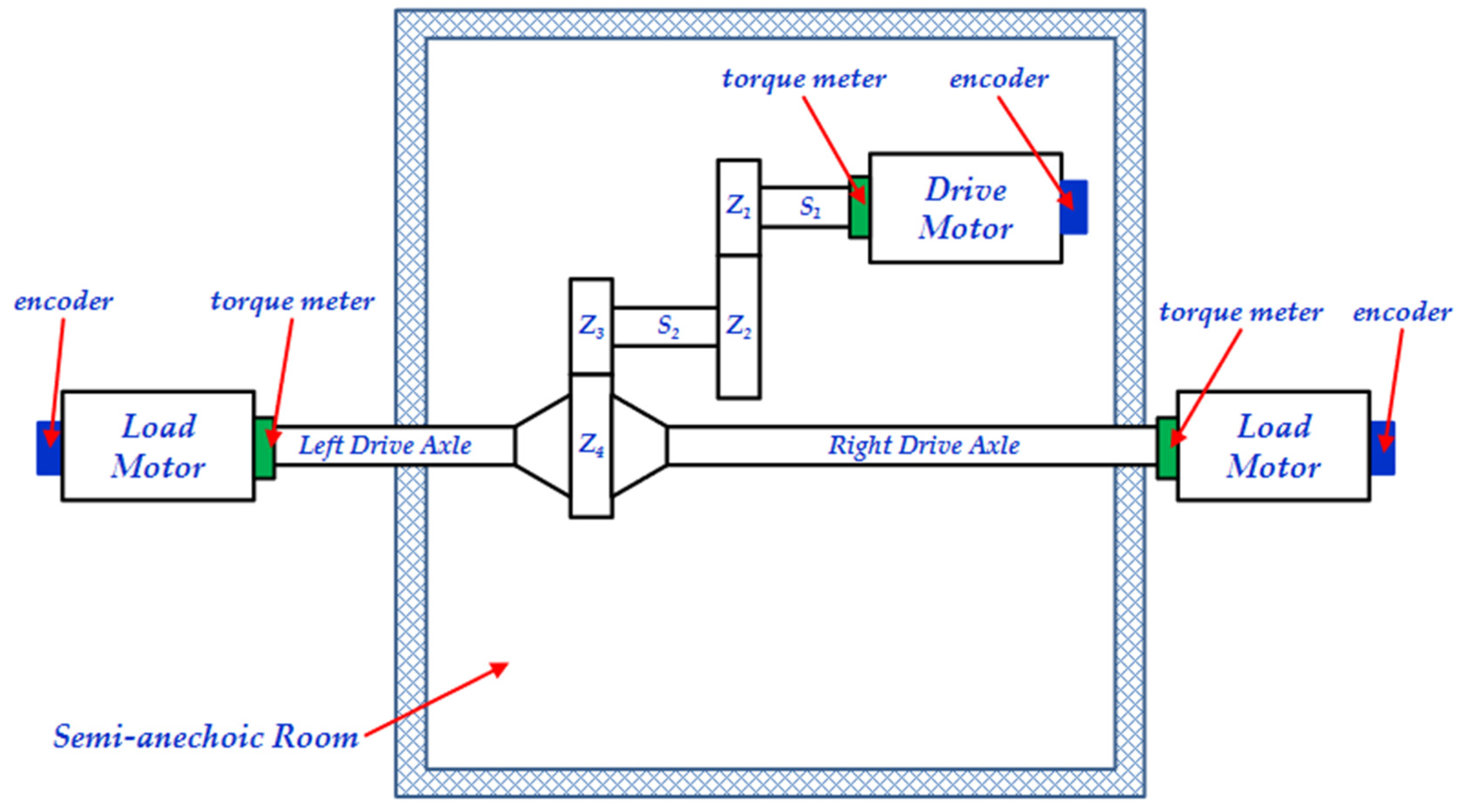
3. Experimental Test and Measurement

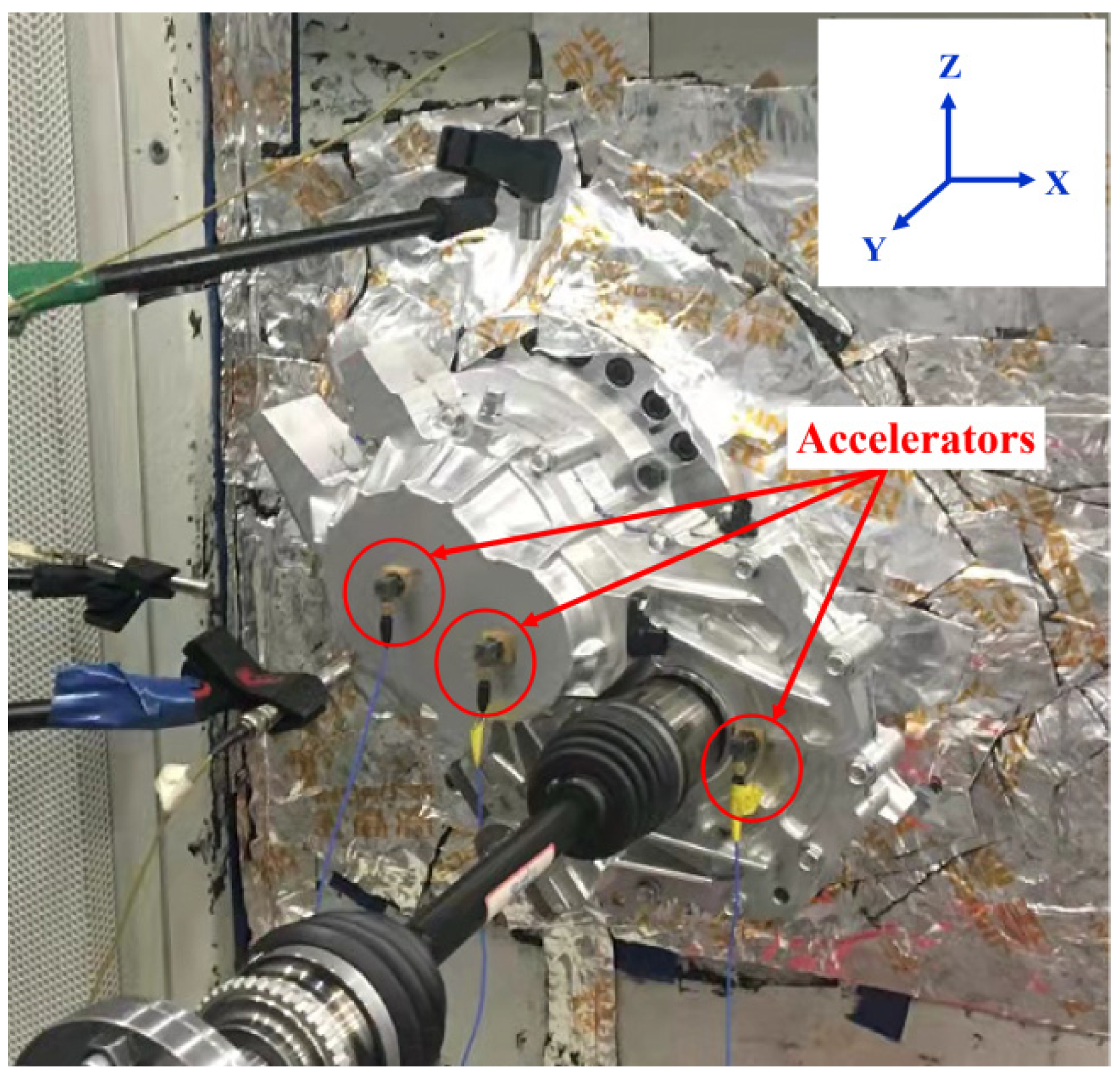
3.1. Test Equipment

The experiment was carried out in the semi-anechoic room, and the test rig layout is shown in Figure 6. The test rig mainly consists of five motors; four of them are the load motors and the center one is the drive motor. The four load motors can be moved horizontally and longitudinally to form a wheel base range of 2000~4500 mm, and a wheel track range of 1200~2000 mm. In this work, only two load motors were used.

The drive motor had a rated power of 220 kW, a rated torque of 450 Nm, and maximum speed of 10,000 rpm. The load motor had a rated power of 355 kW, a rated torque of 4000 Nm, and maximum speed of 3000 rpm. Each motor was equipped with an encoder and a torque meter to measure its rotation speed and torque.

Besides the test rig, three accelerators of PCB 356A33 were used to collect test data, one 48 channel data acquisition equipment of LMS SCL 220 was used to record test data, and the software of LMS Test Lab 14A was used to process test data.

3.2. Test Method

The analysis bandwidth was set to 5120 Hz, and the resolution was set to 1 Hz. Figure 7 shows the housing vibration measurement positions and measurement coordinate setting. Three accelerators were respectively mounted on the transmission housing surface to measure the positions of input shaft, intermediate shaft, and output shaft vibration accelerations. The coordinate system was set as follows: the direction from input shaft to output shaft was positive X, the direction perpendicular to the ground was positive Z, and the direction generated by the right-hand rule was positive Y.

4. Results and Discussion

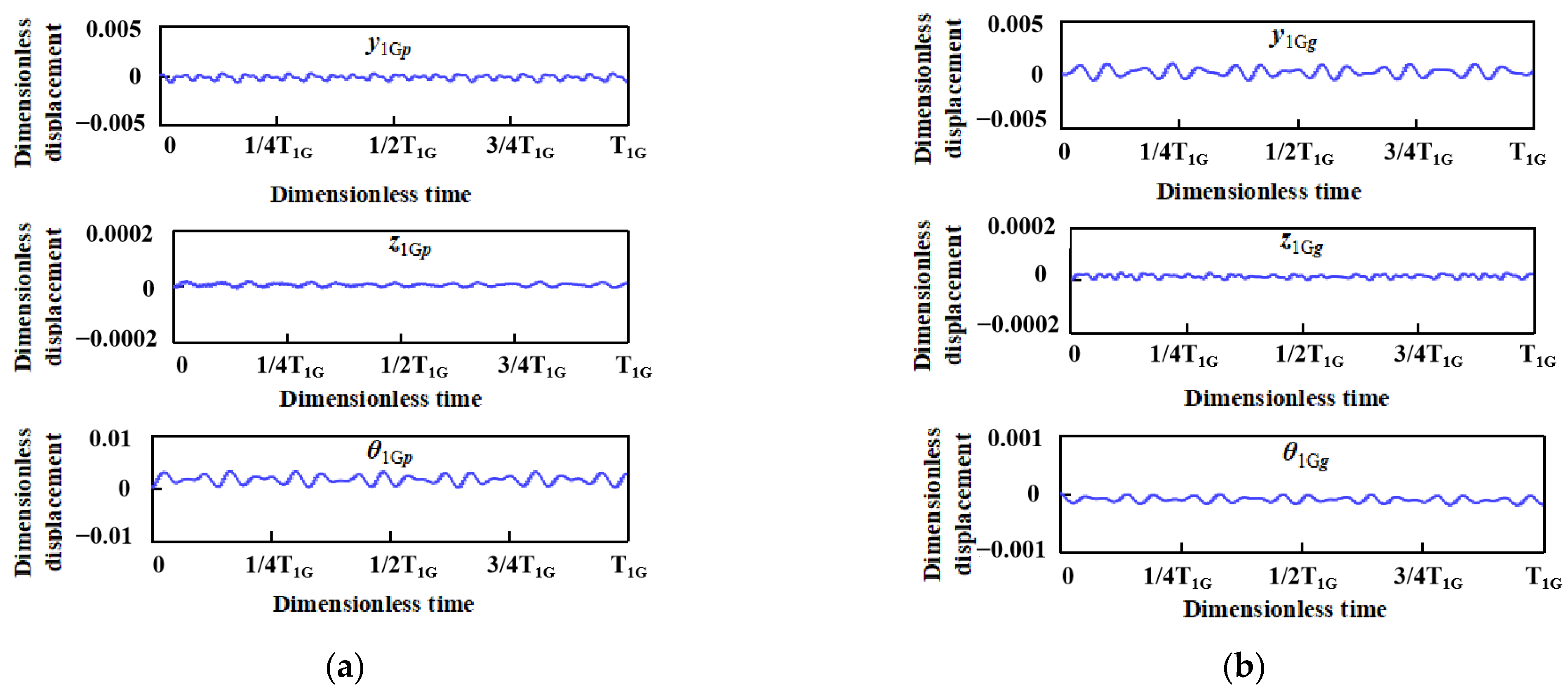
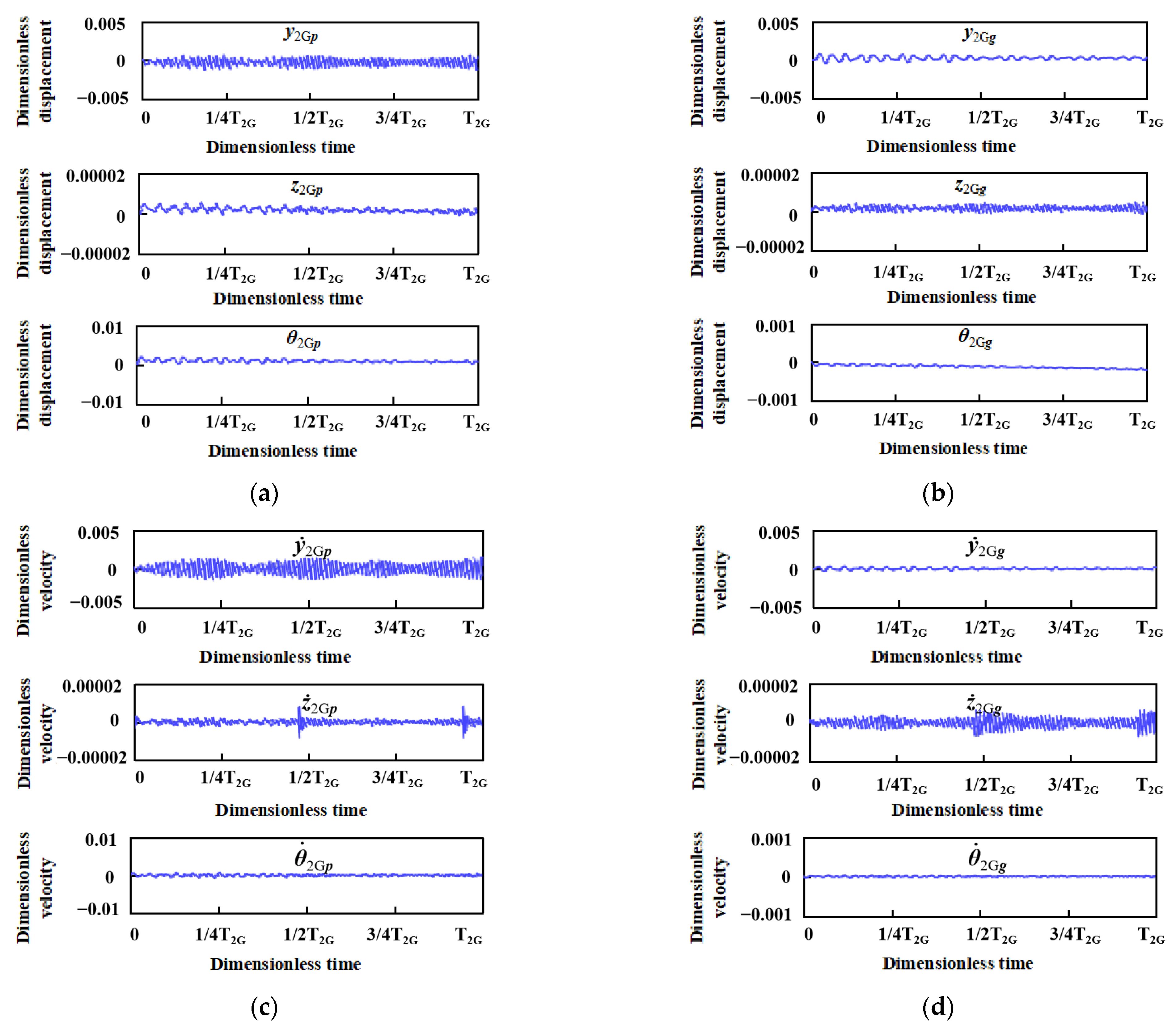
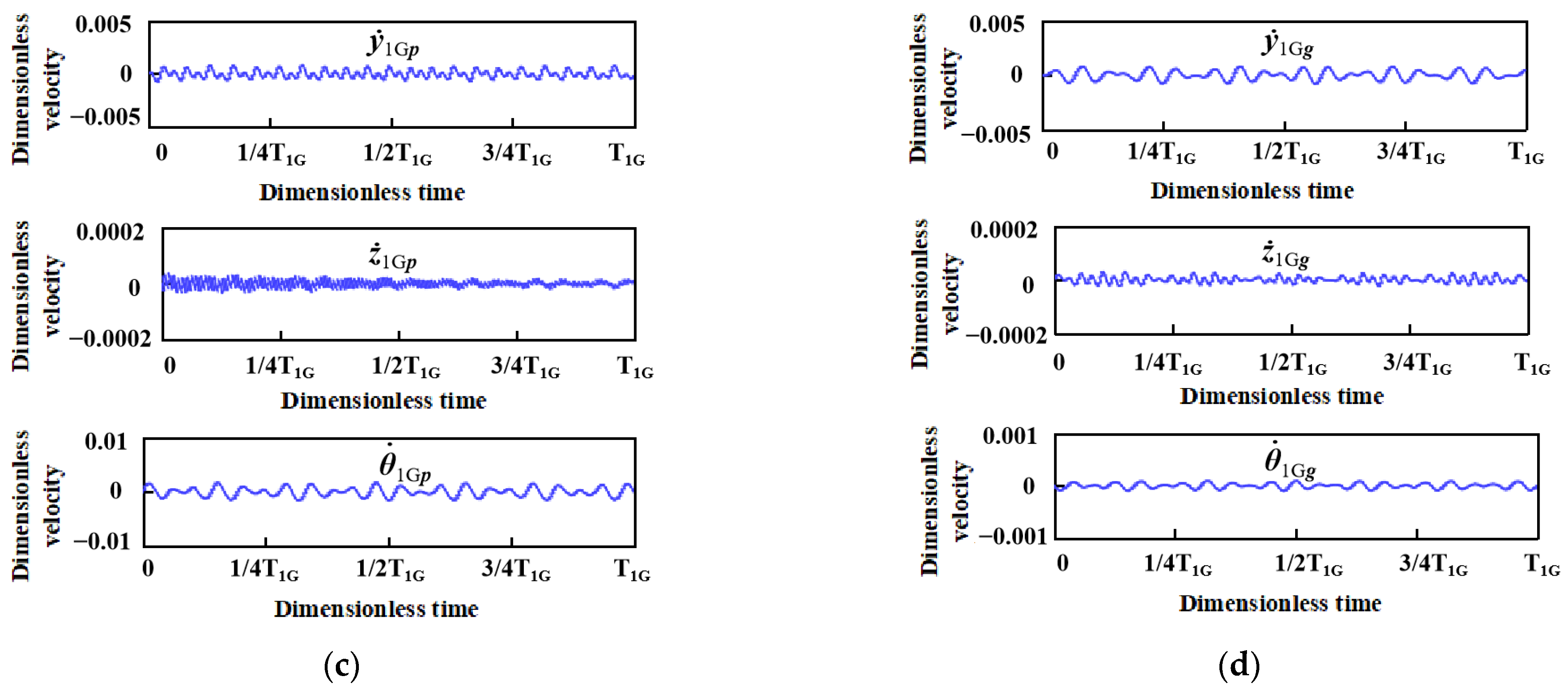
4.1. State Space Calculation

In order to improve the calculation efficiency and attribute different physical quantities on the same scale, the dynamic equation in Section 2.1 was processed by the dimensionless method. Taking the condition of 3000 rpm and 60 Nm as an example, the state space changing process of the first-stage gear pair Z₁ and Z₂ is shown in Figure 8, and the state space changing process of the second-stage gear pair Z₃ and Z₄ is shown in Figure 9.

The results shown in Figure 8 and Figure 9 include the tangential, axial, and torsional vibration displacement and vibration velocity of the driving gear and driven gear.

In terms of the changing process, all variables show regular oscillation. The meshing cycle of the first-stage gear pair was 0.001818 s, and the meshing cycle of the second-stage gear pair was 0.003850 s. Therefore, 2.11 times the input periodic excitation of the first-stage gear pair was included in one meshing cycle of the second-stage gear pair. This feature can be clearly seen from Figure 9c,d, in that there are two speed mutations.

In terms of amplitude, the tangential vibration of the two pairs of gears is greater than the axial vibration, and the torsional vibration of the driving gear is greater than that of the driven gear. Comparing Figure 8 with Figure 9, the vibration amplitudes of the first-stage gear pair are greater than those of the second-stage gear pair. This indicates that in the time domain, the vibration of the first-stage gear pair is greater than that of the second-stage gear pair. The above inference is confirmed by the test data that the overall vibration acceleration of the input shaft is indeed greater than that of the output shaft.

From the aspect of frequency, the time domain signal of each pair of gear variables contains a variety of frequency features, which means the dynamic meshing force is composed of peaks with various frequencies.

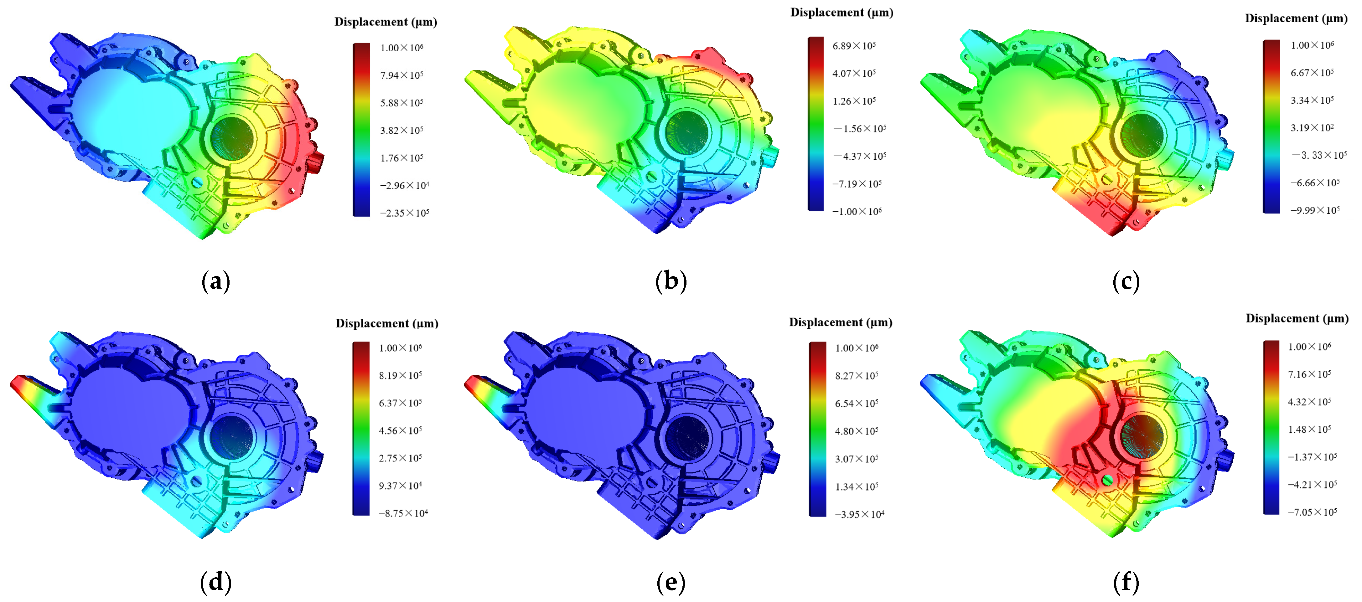
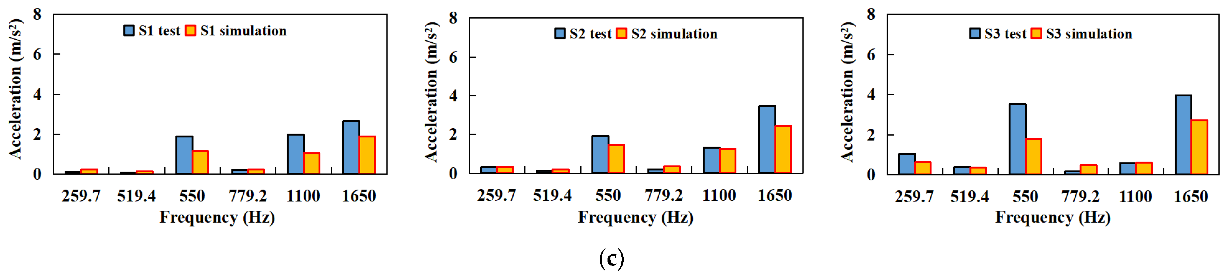
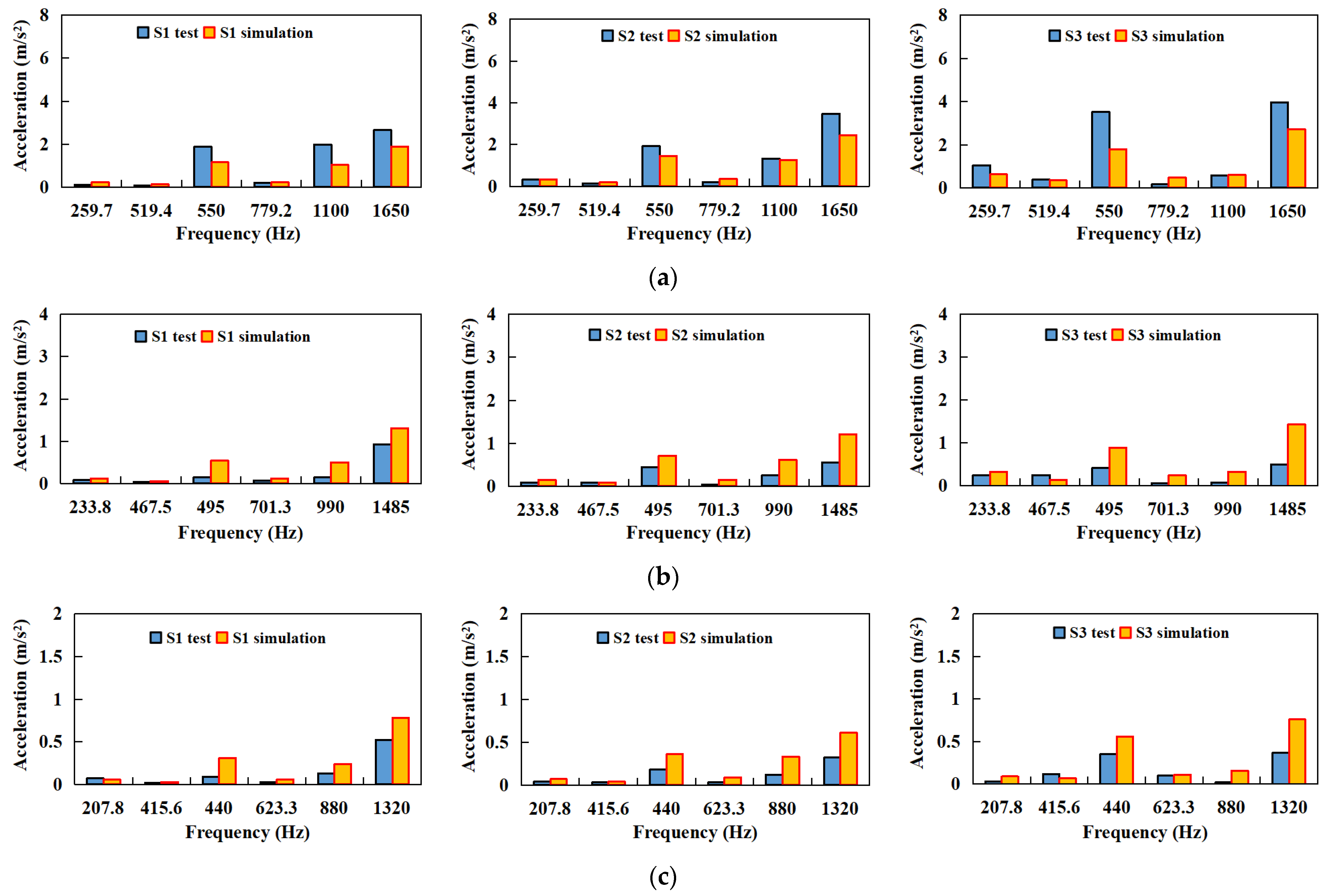
4.2. Transmission Housing Vibration Response

In order to further study the vibration characteristics of the gear system and verify the correctness of the gear system dynamic model and the state space solution method, the dynamic meshing force generated by the calculation was applied to the finite element model of the transmission housing to solve the vibration acceleration of the housing. The simulation results were compared with the measured vibration acceleration.

Generally, the vibration acceleration sensor mainly collects the vibration signals in the three directions of X, Y, Z on the housing surface. Through the comparative analysis of the experimental data, the axial vibration is the main characteristic of the transmission vibration. Therefore, this paper focuses on the axial vibration to conduct the theoretical calculation, experimental validation, and discussion of results.

The axial dynamic meshing force of the transmission gear system was solved based on Equation (8). By using the fast Fourier transform (FFT) method [29], the excitation force can be transformed into the frequency domain and then loaded into the transmission housing FE model. The axial dynamic meshing force spectrum of input shaft, intermediate shaft, and output shaft in the condition of 3000 rpm and 60 Nm was obtained and is shown in Figure 10.

It can be seen that in Figure 10, the frequency features of the input shaft and output shaft are mainly the components of gear meshing fundamental frequency and its multiples. For the input shaft, the fundamental frequency is 550 Hz, and for output shaft, the fundamental frequency is 259.7 Hz. However, for the intermediate shaft, its frequency features are relatively complex due to the coupling effects of both the first-stage gear pair dynamic force and the second-stage gear pair dynamic force. Thus, the frequency features of the intermediate shaft contain both 550 Hz and 259.7 Hz and their multiples.

In order to analyze the vibration acceleration distribution of the transmission, the housing modal analysis was solved by finite element method [30,31]. The finite element model of transmission housing was constrained by its connection side with the drive motor. The material of the housing was aluminum alloy, with a modulus of elasticity of 71 GPa, Poisson’s ratio of 0.33, and density of 2700 kg/m³. The first six modal shapes of the transmission housing are shown in Figure 11.

Different torques of 90, 75, and 60 Nm and three working conditions with the same torque of 60 Nm, and different speeds of 2400, 2700, and 3000 rpm were selected to solve the simulation model and were compared with the test data. The results are shown in Figure 12 and Figure 13.

Figure 12 and Figure 13 show the comparison of housing vibration acceleration under the fundamental gear meshing frequency and its second and third harmonic frequencies of the first-stage gear pair and second-stage gear pair.

In terms of vibration frequency, the simulation results and the test results are matched perfectly, which proves that there is no problem in the signal processing.

In terms of vibration amplitude, since the vibration amplitude of the second-stage gear pair under the first three meshing frequencies is small, there is little difference between the simulation results and the test results, so it is in good agreement. For the first-stage gear pair, the vibration amplitude under the first three meshing frequencies is large, and the simulation model is far less complex than the test conditions, so the amplitude cannot be perfectly corresponding. However, from the overall trend, the simulation results are generally consistent with the test results.

In terms of working conditions, the vibration accelerations of input shaft, intermediate shaft, and output shaft change little under the constant speed but changing torque conditions, indicating that the change of torque has little effect on the housing vibration. Under the constant torque but changing speed conditions, the vibration accelerations of input shaft, intermediate shaft, and output shaft changes obviously, indicating that the change of speed has a great impact on the housing vibration. As a result, the housing vibration is more sensitive to the frequency of excitation rather than the amplitude of excitation.

Through the comparative analysis of the above simulation and test, it is regarded that the simulation results can reflect the main vibration characteristics of the transmission gear system. Therefore, the improved dynamic model of the gear system, as well as the state space method described in Section 2, are proved reliable and universal.

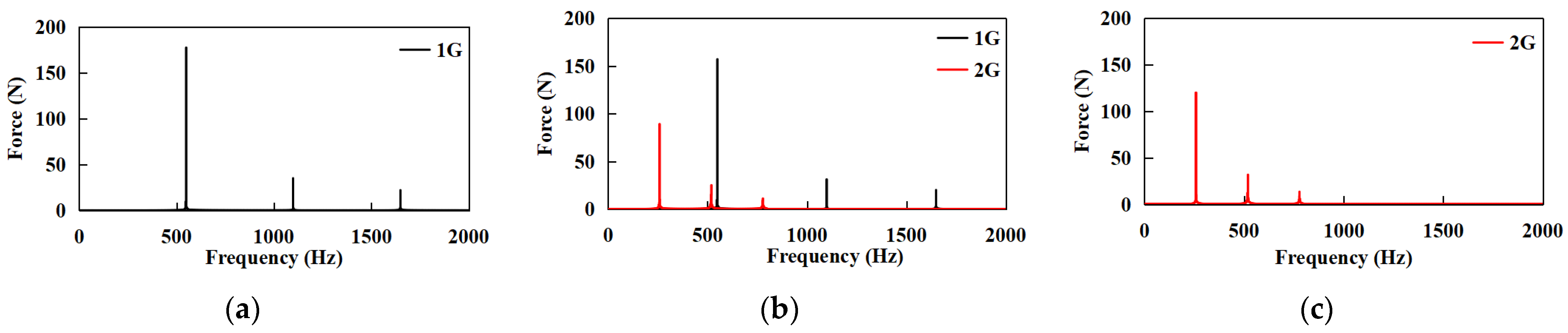
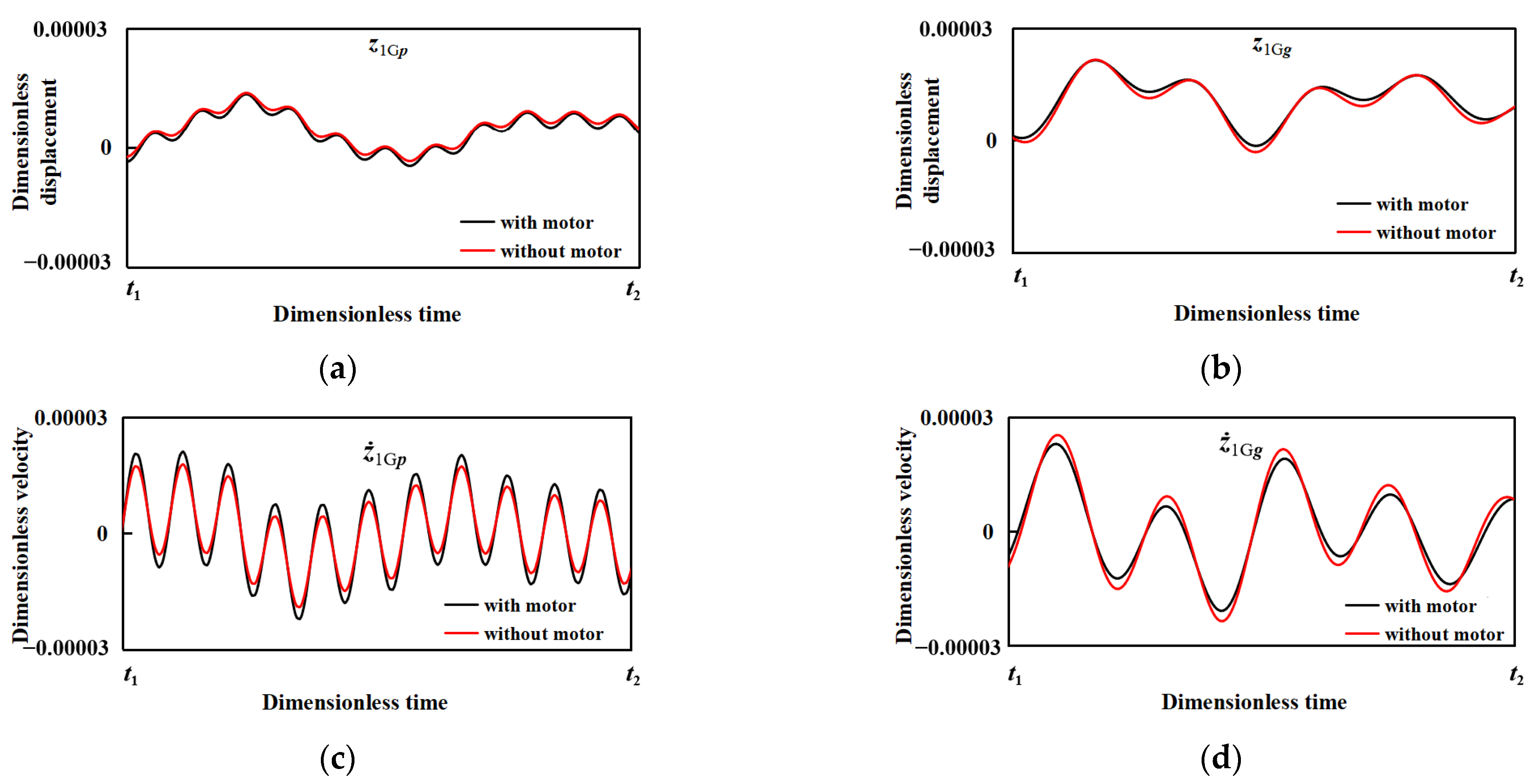
4.3. Influence of Motor Excitation

For the electric vehicle transmission gear system, motor excitation is no doubt a significant factor which determines the vibration response of transmission gears. The effect of motor torque fluctuation on gear vibration response has been studied in [32]. The results indicate that vibration amplitudes are increased at certain modes of gears. In this work, the effect of motor axial force was investigated to illustrate the influence mechanism on gear meshing axial vibration.

According to the dynamic model of the gear system established in Section 2.1, the gear system vibration changing process, with and without motor excitation, was calculated. Figure 14 shows the comparison of the axial vibration displacement and vibration velocity of the first-stage gear pair Z₁ and Z₂ with and without drive motor excitation at 3000 rpm 60 Nm. In order to clearly show the comparison results, a small change process from t₁ to t₂ is intercepted in Figure 14.

It can be seen from Figure 14 that the vibration displacement and vibration velocity of the driving gear Z₁ with motor excitation are larger than those without motor excitation. On the contrary, for the driven gear Z₂, the amplitude of vibration displacement and vibration velocity are decreased.

Formulas (13) and (16) describe the axial force equations of driving gear Z₁ and driven gear Z₂. On the right side of the formulas, the axial forces on both the driving gear and driven gear are expressed. They are equal but with opposite directions. On the left side of the formulas, the coupling of mass, stiffness, damping, and variables are expressed. Since the driving gear on the input shaft is directly connected with the motor shaft, the motor excitation strengthens the vibration characteristics of the driving gear. For the driven gear, under the condition of dynamic equilibrium set by Formulas (13) and (16), the amplitude of vibration displacement and vibration velocity of the driven gear decreases correspondingly.

In summary, this section calculates the comparison of vibration displacement and vibration velocity of gears with and without motor excitation and reveals the influence of the motor excitation on the vibration characteristics of the gear system. The dynamic model of the gear system and the state space solution method could be further used in motor electromagnetic force investigations and gear vibration friction research.

5. Conclusions

An improved dynamic model of the motor-gear system was established. The model contains the tangential, axial, and torsional variables of each gear, considers the influence of the motor and load, and realizes the correlation of the two-stage gear pairs. The improved model more closely fits the actual situation, which possesses important value in electric vehicle industry.

The state space method was used to solve the dynamic model of the motor-gear system. This method is suitable for solving the complex dynamic model and can quickly calculate the numerical solutions of multiple degree of freedom vibration equations. The changing process of each variable was also revealed. It overcomes the shortcomings of other numerical methods, such as the difficultly in solving multiple variables and lack of time processing.

The influence of motor excitation on the state space of the motor-gear system was discussed. The results indicate that motor excitation impacts the vibration displacement and vibration velocity of both the driving gear and driven gear. As a consequence, the dynamic model of the motor-gear system and state space solution method could be further used for motor electromagnetic force investigations and gear vibration research.

References

1. Chen, R.; Zhou, J.; Sun, W. Dynamic characteristics of a planetary gear system based on contact status of the tooth surface. J. Mech. Sci. Technol. 2018, 32, 69–80. [Google Scholar] [CrossRef]
2. Luo, B.; Li, W. Experimental study on thermal dynamic characteristics of gear transmission system. Measurement 2019, 136, 154–162. [Google Scholar] [CrossRef]
3. Zhu, C.; Xu, X.; Liu, H.; Luo, T.; Zhai, H. Research on dynamical characteristics of wind turbine gearboxes with flexible pins. Renew. Energy 2014, 68, 724–732. [Google Scholar] [CrossRef]
4. Guo, D.; Zhou, Y.; Wang, Y.; Chen, F.; Shi, X. Numerical and experimental study of gear rattle based on a refined dynamic model. Appl. Acoust. 2022, 185, 108407. [Google Scholar] [CrossRef]
5. Cao, Z.; Chen, Y.; Zang, L. Model-based transmission acoustic analysis and improvement. Proc. Inst. Mech. Eng. Part D J. Automob. Eng. 2020, 234, 1572–1584. [Google Scholar] [CrossRef]
6. Wei, S.; Zhao, J.; Han, Q.; Chu, F. Dynamic response analysis on torsional vibrations of wind turbine geared transmission system with uncertainty. Renew. Energy 2015, 78, 60–67. [Google Scholar] [CrossRef]
7. Inalpolat, M.; Handschuh, M.; Kahraman, A. Influence of indexing errors on dynamic response of spur gear pairs. Mech. Syst. Signal Process. 2015, 60–61, 391–405. [Google Scholar] [CrossRef]
8. Duan, T.; Wei, J.; Zhang, A.; Xu, Z.; Lim, T.C. Transmission error investigation of gearbox using rigid-flexible coupling dynamic model: Theoretical analysis and experiments. Mech. Mach. Theory 2021, 157, 104213. [Google Scholar] [CrossRef]
9. Garambois, P.; Perret-Liaudet, J.; Rigaud, E. NVH robust optimization of gear macro and microgeometries using an efficient tooth contact model. Mech. Mach. Theory 2017, 117, 78–95. [Google Scholar] [CrossRef] [Green Version]
10. Wang, J.; He, G.; Zhang, J.; Zhao, Y.; Yao, Y. Nonlinear dynamics analysis of the spur gear system for railway locomotive. Mech. Syst. Signal Process. 2017, 85, 41–55. [Google Scholar] [CrossRef]
11. Wang, X. Stability research of multistage gear transmission system with crack fault. J. Sound Vib. 2018, 434, 63–77. [Google Scholar] [CrossRef]
12. Abboudi, K.; Walha, L.; Driss, Y.; Maatar, M.; Fakhfakh, T.; Haddar, M. Dynamic behavior of a two-stage gear train used in a fixed-speed wind turbine. Mech. Mach. Theory 2011, 12, 1888–1900. [Google Scholar] [CrossRef]
13. Walha, L.; Driss, Y.; Khabou, M.T.; Fakhfakh, T.; Haddar, M. Effects of eccentricity defect on the nonlinear dynamic behavior of the mechanism clutch-helical two stage gear. Mech. Mach. Theory 2011, 7, 986–997. [Google Scholar] [CrossRef]
14. Cai, Y.; Hayashi, T. The Linear Approximated Equation of Vibration of a Pair of Spur Gears (Theory and Experiment). J. Mech. Des. 1994, 116, 558–564. [Google Scholar] [CrossRef]
15. Cai, Y. Simulation on the Rotational Vibration of Helical Gears in Consideration of the Tooth Separation Phenomenon (A New Stiffness Function of Helical Involute Tooth Pair). J. Mech. Des. 1995, 117, 460–469. [Google Scholar] [CrossRef]
16. Wei, J.; Zhang, A.; Wang, G.; Qin, D.; Lim, T.C.; Wang, Y.; Lin, T. A study of nonlinear excitation modeling of helical gears with Modification: Theoretical analysis and experiments. Mech. Mach. Theory 2018, 128, 314–335. [Google Scholar] [CrossRef]
17. Wu, X.; He, H.; Chen, G. A new state-space method for exponentially damped linear systems. Comput. Struct. 2019, 212, 137–144. [Google Scholar] [CrossRef]
18. Lu, K.; Zhou, W.; Zeng, G.; Du, W. Design of PID controller based on a self-adaptive state-space predictive functional control using extremal optimization method. J. Frankl. Inst. 2018, 355, 2197–2220. [Google Scholar] [CrossRef]
19. Demirhan, P.A.; Taskin, V. Bending and free vibration analysis of Levy-type porous functionally graded plate using state space approach. Compos. Part B Eng. 2019, 160, 661–676. [Google Scholar] [CrossRef]
20. Vaseghi, N.; Abrishamian, M.S. Analysis of electromagnetic scattering from anisotropic cylindrical structures using state space method. AEU-Int. J. Electron. Commun. 2018, 89, 24–33. [Google Scholar] [CrossRef]
21. Scheel, M.; Kleyman, G.; Tatar, A.; Brake, M.R.W.; Peter, S.; Noël, J.-P.; Allen, M.S.; Krack, M. Experimental assessment of polynomial nonlinear state-space and nonlinear-mode models for near-resonant vibrations. Mech. Syst. Signal Process. 2020, 143, 106796. [Google Scholar] [CrossRef]
22. Fang, Y.; Zhang, T.; Yu, P.; Guo, R. Effect of tangential electromagnetic force on vibration and noise of electric powertrain. Electric Mach. Control 2016, 20, 90–95. [Google Scholar]
23. Li, B. Calculation Method for Axial Force of Motor Based on Two-dimensional Electromagnetic Field Simulation. Micromotors 2019, 52, 28–33. [Google Scholar]
24. Chen, S.; Tang, J.; Wu, L. Dynamics analysis of a crowned gear transmission system with impact damping: Based on experimental transmission error. Mech. Mach. Theory 2014, 74, 354–369. [Google Scholar] [CrossRef]
25. Amabili, M.; Fregolent, A. A method to identify modal parameters and gear errors by vibrations of a spur gear pair. J. Sound Vib. 1998, 214, 339–357. [Google Scholar] [CrossRef]
26. Chang, L.; He, Z.; Liu, G. A generalized dynamic model for parallel shaft gear transmissions and the influences of dynamic excitations. J. Vib. Shock 2016, 35, 7–14. [Google Scholar] [CrossRef]
27. Alptekin, A.; Broadstock, D.C.; Chen, X.; Wang, D. Time-varying parameter energy demand functions: Benchmarking state-space methods against rolling-regressions. Energy Econ. 2019, 82, 26–41. [Google Scholar] [CrossRef]
28. Ding, Z.; Li, L.; Hu, Y.; Li, X.; Deng, W. State-space based time integration method for structural systems involving multiple nonviscous damping models. Comput. Struct. 2016, 171, 31–45. [Google Scholar] [CrossRef]
29. Zandi-Mehran, N.; Nazarimehr, F.; Rajagopal, K.; Ghosh, D.; Jafari, S.; Chen, G. FFT bifurcation: A tool for spectrum analyzing of dynamical systems. Appl. Math. Comput. 2022, 422, 126986. [Google Scholar] [CrossRef]
30. Han, J.; Liu, Y.; Yu, S.; Zhao, S.; Ma, H. Acoustic-vibration analysis of the gear-bearing-housing coupled system. Appl. Acoust. 2021, 178, 108024. [Google Scholar] [CrossRef]
31. Xu, B.; Ye, S.; Zhang, J. Numerical and experimental studies on housing optimization for noise reduction of an axial piston pump. Appl. Acoust. 2016, 110, 43–52. [Google Scholar] [CrossRef]
32. Wang, Y.; Liao, Y.; Xu, H. Effects of multi-excitation on vibration characteristics of planetary gear system. Alex. Eng. J. 2022, 61, 10593–10602. [Google Scholar] [CrossRef]
Figure 1. The dynamic model of the motor-gear system: (a) the layout of the motor-gear system; (b) the gear meshing dynamics without taking into account the frictional forces.
Machines 10 00589 g001
Figure 2. Length of contact line in meshing plane of helical gear: (a) εαεβ; (b) εα > εβ.
Machines 10 00589 g002
Figure 3. Single tooth meshing stiffness comparison between Cai’s method and proposed method.
Machines 10 00589 g003
Figure 4. Meshing stiffness contains multiple pairs of teeth meshing.
Machines 10 00589 g004
Figure 5. Structure diagram of MIMO linear time-varying system.
Machines 10 00589 g005
Figure 6. Test rig layout and measurement method.
Machines 10 00589 g006
Figure 7. Housing vibration measurement positions and measurement coordinate setting.
Machines 10 00589 g007
Figure 8. State space of the first-stage gear pair Z1 and Z2: (a) vibration displacement of driving gear; (b) vibration displacement of driven gear; (c) vibration velocity of driving gear; (d) vibration velocity of driven gear.
Machines 10 00589 g008aMachines 10 00589 g008b
Figure 9. State space of the first-stage gear pair Z3 and Z4: (a) vibration displacement of driving gear; (b) vibration displacement of driven gear; (c) vibration velocity of driving gear; (d) vibration velocity of driven gear.
Machines 10 00589 g009
Figure 10. Axial dynamic meshing force spectrum: (a) input shaft spectrum; (b) intermediate shaft spectrum; (c) output shaft spectrum.
Machines 10 00589 g010
Figure 11. Modal shapes of the transmission housing under different frequencies with constraint: (a) 834 Hz; (b) 840 Hz; (c) 1752 Hz; (d) 2121 Hz; (e) 2524 Hz; (f) 2588 Hz.
Machines 10 00589 g011
Figure 12. Comparison between simulation results and test data of housing vibration: (a) 3000 rpm 90 Nm input shaft, intermediate shaft, and output shaft accelerations; (b) 3000 rpm 75 Nm input shaft, intermediate shaft, and output shaft accelerations; (c) 3000 rpm 60 Nm input shaft, intermediate shaft, and output shaft accelerations.
Machines 10 00589 g012aMachines 10 00589 g012b
Figure 13. Comparison between simulation results and test data of housing vibration: (a) 3000 rpm 60 Nm input shaft, intermediate shaft, and output shaft accelerations; (b) 2700 rpm 60 Nm input shaft, intermediate shaft, and output shaft accelerations; (c) 2400 rpm 60 Nm input shaft, intermediate shaft, and output shaft accelerations.
Machines 10 00589 g013
Figure 14. Comparison of the first-stage gear pair vibration curves with and without motor excitation: (a) gear Z1 vibration displacement curves; (b) gear Z2 vibration displacement curves; (c) gear Z1 vibration velocity curves; (d) gear Z2 vibration velocity curves.
Machines 10 00589 g014